The Distance to NGC 5904 (M 5) via the Subdwarfs Main Sequence Fitting Method

We present a determination of the distance modulus of the globular cluster NGC 5904 (M 5), obtained by means of the subdwarf main–sequence fitting on the (V,V$-$I) color–magnitude diagram. The subdwarf sample has been selected from the HIPPARCOS catalog in a metallicity range homogeneous with the cluster ([Fe/H] $\simeq$ $-$1.1). Both the cluster and the subdwarfs have been observed with the same telescope+instrument+filters setup (namely, ESO–NTT equipped with the SUSI2 camera), in order to preserve homogeneity and reduce systematic uncertainties. A set of archival HST data has then been used to obtain a deep and precise ridge line. These have been accurately calibrated in the ground photometric system by using the NTT data and used to fit the cluster distance modulus. By adopting the most commonly accepted values for the reddening, E(B$-$V) = 0.035 and 0.03, we obtain respectively $\mu_{0}=14.44\pm 0.09\pm 0.07$ and $\mu_{0}=14.41\pm 0.09\pm 0.07$, in agreement with recent determinations.

1 Introduction

The ages of the Galactic Globular Clusters (hereafter GGCs) represent one of the milestones on the road of our comprehension of the Universe. In order to derive reliable absolute ages estimates, the most important parameter to determine is the distance (see Renzini, 1991). Errors on the distance propagates through the age determination procedure in such a way that a 0.08 error in the distance modulus (DM) propagates as a 12% error in the age. Different ages (younger or older) mean different epoch of formation of the Galaxy. Therefore, it can be easily seen how the uncertainty in GGCs ages estimates significantly affects models of galaxy formation and cosmological evolution.

The recent availability of the HIPPARCOS catalog of trigonometric parallaxes (Perryman et al., 1997) has greatly improved the knowledge of GGCs distances. A large number of papers on the subject have been published since then (e.g. Reid, 1997; Gratton et al., 1997; Pont et al., 1998; Vandenberg et al., 2002; Gratton et al., 2003), most of which present larger distances, and hence younger ages, with respect to previous works (with the exception, among the cited works, of Pont et al., 1998, who recover the pre-Hipparcos results of 1992).

The method used consists of a fit of the cluster main sequence to the subdwarfs main-sequence of corresponding metallicity, once the reddening has been subtracted. This procedure is, of course, prone to uncertainties, both random and systematic: on the subdwarf side errors on parallax measurements, Lutz-Kelker correction, metallicity; on the cluster side reddening, metallicity, narrowness and accuracy of the mean ridge line. A further effect is represented by the presence of binary stars in the cluster CMD and in the subdwarfs sample. In the first case the determination of the mean ridge line is altered, if a proper fitting procedure is not taken into account. In the second, the magnitude of the field star is different from stars of analogous metallicity. This issue has been widely discussed in, e.g., Gratton et al. (1997); Pont et al. (1998); Carretta et al. (2000), and will be analyzed in detail later. If HIPPARCOS gave the chance to significantly reduce the random errors on parallax measurements, nonetheless other sources of errors still remain. Metallicity, for example, represents a common problem that significantly affects the determination of the distance modulus, because of either the spread in metallicity of the sequence of local subdwarfs or the error on the absolute values. There are two strategies to go around this problem: to obtain a sufficiently large set of subdwarfs in the right metallicity range, or to apply a relation that transforms the colors of the stars of different metallicity. The second introduces a model-dependent relation and should be used with caution. Of course, the first solution is better, especially if the sample of subdwarfs draws a main sequence down to very low masses. In fact, recent HST color-magnitude diagrams of GGCs reach very faint magnitudes, hence small masses, but a similar sequence for subdwarfs is currently not available. Reid and Gizis (1998) fit a distance modulus to NGC 6397 by using a sequence of lower MS subdwarfs, but their work stands on the fact that the sequence of very metal-poor subdwarfs define a reasonably narrow sequence. This is not true, instead, for subdwarfs of higher metallicities (see their Fig. 2). On the other hand, the most widely used set of subdwarfs cover magnitudes ranging from $\mathrm{M}_{V}\sim 7$ and brighter, leaving uncovered the range between this value and the extreme subdwarfs. This is explained with the relative lack of halo stars near the Sun (Reid and Gizis, 1998). One of the possibilities we discuss in order to reduce the uncertainties is to perform a uniform study of a subdwarfs sample and a GGC by using the same telescope, instrumentation and, possibly, observing nights, thus eliminating the systematics due to the relative calibrations among different instrumental setups. For this reason, we observed the target cluster and a sample of subdwarfs in the proper metallicity range matching the cluster’s with the same telescope+instrument (NTT+SUSI2) and then used archival data from HST to go faint and calibrated the HST magnitudes into the ground system, obtaining a deep and fully homogenous data set. The selected object is the well known cluster NGC 5904 (M 5), for which a wide set of photometric and spectroscopic studies is available in the literature. Moreover, Sandquist et al. (1996, S96), Reid (1997), Gratton et al. (1997), Chaboyer et al. (1998) and, more recently, Vandenberg et al. (2002) determined the DM of the cluster by using the trigonometric parallaxes of subdwarfs and various sets of models. These works will be often referred to in the following.

NGC 5904 is a typical old halo cluster of intermediate metallicity -[Fe/H] $\sim-1.1$ in the scale of Carretta and Gratton (1997) (CG), $-$1.4 in the Zinn and West (1984) scale (ZW). A recent study of Ramirez and Cohen (2003) gives [Fe/H] $\simeq-1.3$. The morphology of the horizontal branch (HB) does not show signs of the second parameter effect and several age determinations are available. The structure of the paper is outlined as follows: Sect. 2 describes the observations and the archival material, Sect. 3 presents the reduction and calibration of the data, in Sect. 4 we present and analyze the subdwarfs sample. In Sect. 5 the cluster color-magnitude diagram (CMD) is presented and discussed, and in Sect. 6 the DM-fit is analyzed. In Sect. 7 a final discussion is summarized.

2 Data Set

2.1 Observations

Observations have been performed with the ESO-NTT telescope equipped with SUSI2 as a backup program during three different campaigns, in december 1999 (63.L-0717, subdwarfs + cluster), december 2000 (66.D-0242, subdwarfs), february 2002 (68.B-0061, cluster). The adopted strategy was to observe both the subdwarfs sample and the target cluster with the same setup telescope+instrument+filters+detector and, possibly, within the same campaign, in order to remove any systematics due to the use of different setups. The december 1999 and february 2002 campaigns produced very good quality data, while the december 2000 set (two subdwarfs only) presented moderately poor photometric conditions. Seeing was not a major problem for observing the subdwarfs,because they had to be defocussed in order not to saturate the chip. This, coupled to the fact that the objects were observed in the central region of the frames, allowed to use exposure times long enough to have a negligible shutter effect. The typical observing time, per frame, was 0.5 s.

The data set for the target cluster (NGC 5904 = M 5) was secured in december 1999, when the seeing was poor, together with the subdwarfs, and in february 2002 when seeing was considerably better, in order to have a comparison data-set. In both cases, the run was found to be photometric and, in fact, the run-to-run scatter in the magnitudes is almost absent, without any trend in the magnitudes and colors (see Fig 5). The field was selected 2 arcmin North of the cluster center, to ensure an almost complete overlapping with the field observed with HST that have been retrieved from the archive (see below). Only images in V and I bands for the cluster were taken, because the space-based data-set consists of images in these two bands only. For the subdwarfs, also B frames were secured.

2.2 Archival data

A set of deep exposures was available from the STScI HST WFPC2 archive (GO 8310), in the two wide bands F555W (V) and F814W (I). A total of 6 F555W and 9 F814W frames were retrieved from the archive, and pre-reduced by using the HST pipeline, available in STSDAS running under IRAF (Tody, 1986, 1993), and using the most recent calibration frames and tables (see the WFPC2 web page for details).

3 Reductions and Calibrations

3.1 Reductions

Reductions have been done for all the data-sets by using IRAF and the digiphot packages daophot and photcal for building up the catalog and apply photometric calibrations respectively. In particular, since the telescope had been defocused when observing the subdwarfs sample, for these stars aperture photometry has been used. For cluster images, both NTT and HST, we applied the standard daophot PSF fitting routines. In particular, the NTT data-set is characterized by a relatively high oversampling (FWHM $\sim$ 5 pix), and in this case a gaussian model for the PSF plus look-up table of correction varying quadratically along the frames has been used. HST-WFPC2 frames, on the other hand, are undersampled (estimated FWHM $\sim$ 1.6 pix), and in this case a moffat15 function, with quadratic look-up table, gave better results. As a general strategy, object searching has been done independently on each frame, after registering all of them to a common reference frame (the best seeing one). In the case of HST, all the images were almost perfectly registered onto each other, and no shift or rotation was needed. We made use of the world coordinate system available in the FITS header in order to obtain later an astrometric calibration of the catalogs.

3.2 Photometric calibrations

For both data-set, aperture corrections were applied in order to report the PSF magnitudes to aperture magnitudes before calibrating. HST-WFPC2 data were reported to the standard aperture of 0.1^″, following the calibration procedure of (Holtzmann et al., 1995). For ESO-NTT data, growth-curves (from DAOGROW) have been used and aperture corrections at infinity have been computed. For ground-based data, a set of Landolt standards has been secured for each run and calibration equations derived, in the form 3.2. Table 1 reports the calibration coefficients of all the runs. The equation for the V filter has been derived against $\mathrm{B-V}$ in the two first runs, as B,V,I data were available both for subdwarfs and for NGC 5904. In the last run, only NGC 5904 has been observed and only in V and I filters, hence we calibrated the V magnitude against (V-I).

$$v = V+a_{0}+a_{1}\times(b-v)+a_{2}\times X_{V}$$

$$v = V+a_{0}^{\prime}+a_{1}^{\prime}\times(v-i)+a_{2}^{\prime}\times X_{V}$$ (1)

$$b = B+b_{0}+b_{1}\times(b-v)+b_{2}\times X_{B}$$

$$i = I+c_{0}+c_{1}\times(v-i)+c_{2}\times X_{I}$$

Table 1: Calibration coefficients for the three runs.

Filter	Zero Point	Color Term	Extinction
Dec. 1999
B	25.42(0.01)	-0.05(0.01)	0.23(0.01)
V	25.82(0.01)	0.02(0.01)	0.11(0.01)
I	24.74(0.01)	-0.04(0.01)	-0.04(0.01)
Dec. 2000
B	25.86(0.03)	-0.18(0.04)	0.29(0.02)
V	25.94(0.04)	0.00(0.04)	0.19(0.03)
I	24.80(0.01)	-0.17(0.01)	-0.09(0.02)
Feb. 2002
V	25.69(0.01)	-0.01(0.01)	0.15(0.01)
I	24.59(0.02)	-0.03(0.01)	-0.06(0.01)

Figs. 1, 2 and 3 show the difference between standard mags. and calibrated mags. of the Landolt stars used for calibrations in all the runs. As can be seen, the residuals ($\mathrm{Mag}_{std}-\mathrm{Mag}_{fit}$) are on the average very small and with no residual trends with the colors.

Figure 1: Residual between standard magnitudes and calibrated magnitudes for the Landolt stars in the Dec. 1999 run.

Figure 2: Residual between standard magnitudes and calibrated magnitudes for the Landolt stars in the Dec. 2000 run.

Figure 3: Residual between standard magnitudes and calibrated magnitudes for the Landolt stars in the Feb. 2002 run.

The HST-WFPC2 data-set has been calibrated following the procedure describred in Holtzmann et al. (1995). After applying the aperture corrections and correcting for geometric distorsions and CTE effect, following Dolphin (2000), we applied the published coefficients and calibrated the data-set both in the VEGAMAG and STMAG systems. While the V magnitudes are almost identical in the two systems, the I magnitudes differ by a certain amount (around 1.2 mag, depending on the WF chip).

The NTT data-set has then been used to report magnitudes in both system to the ground NTT system, in order to perform also an internal check.

4 The subdwarfs sample

The sample of subdwarfs used for this study has been selected from the HIPPARCOS list taken from the papers of Gratton et al. (1997) and Reid (1997). The requirement was that the sample be as close as possible in metallicity to the target cluster, in order to reduce systematics introduced by any trasformation that would have been needed to report the values to the metallicity of M 5, and be distributed over a wide range of magnitudes and colors in order to overlap a sufficiently large portion of MS and ensure, in this way, a more robust fit to the cluster MS mean ridge line. The sample consists of 6 stars, 4 of which observed in the dec. 1999 run, the others in dec. 2000. Each star has at least three measurements, in order to reduce the error on the magnitudes and remove the effect of eventual bad pixels and/or flat field dishomogeneities.

Since these stars needed to be observed with very short exposure times, the shutter delay of SUSI2 has been taken into account. In particular, the typical exposure time was 0.5s, and the shutter delay for SUSI2, taken from the SUSI2 web page at ESO .

Table 2 shows the calibrated magnitudes and colors for the selected sample. The error indicated is the internal photometric error, and is not representative of the total error. To obtain this last, uncertainties on the reddening and trigonometric parallax must be applied. As pointed out also by Gratton et al. (2003), these stars have virtually zero reddening. The error on the trigonometric parallax, given in the literature, has been applied following the propagation of errors. The Lutz-Kelker correction has been computed on the basis of the discussion by Carretta et al. (2000), by using the formula adopted by the authors (Eq. 1 in the cited work), because the sample had the same selection effect as the one reported in that paper. This value is of the order of 0.02 mag. The associated Malmquist bias, for the same reason, is negligible. By adding all the error sources, the average uncertainty increases to $\sim 0.03$mag but with a spread given by star-to-star differences.

Table 2: The subdwarfs sample

Ident.	B	$\sigma$(B)	V	$\sigma$(V)	I	$\sigma$(I)	[Fe/H]	Mv	$\pi_{mas}$	Run
HIP70681	9.881	0.001	9.302	0.001	8.577	0.001	$-$1.09$\pm$0.07	5.72$\pm$0.16	19.16	Dec99
HIP74234	10.272	0.001	9.422	0.001	8.446	0.001	$-$1.28$\pm$0.07	7.08$\pm$0.11	33.68	Dec99
HIP74235	9.821	0.001	9.059	0.001	$-$	$-$	$-$1.30$\pm$0.07	6.74$\pm$0.08	34.14	Dec99
HIP81170	10.344	0.001	9.611	0.001	8.723	0.001	$-$1.14$\pm$0.07	6.18$\pm$0.15	20.71	Dec99
HIP3026	9.722	0.001	9.269	0.001	8.710	0.001	$-$1.50	4.15	9.57	Dec00
HIP24316	9.924	0.001	9.448	0.001	8.838	0.001	$-$1.44$\pm$0.07	5.28$\pm$0.15	14.55	Dec00

Since the selection has been done with the criterium on the metallicity explained above and requiring that the objects be, of course, visible from the site and in the period of observation, only six subdwarfs have been selected, one of which saturated the I filter even with the shortest possible exposure. The effect of metallicity on the subdwarf fitting to the distance has been extensively discussed by several authors in recent papers (see,e.g., Gratton et al., 1997; Carretta et al., 2000; Gratton et al., 2003; Reid, 1997; Pont et al., 1998) and will not be readdressed here. However, it is worth recalling that by selecting objects with a metallicity close to the cluster’s one, the uncertainities due to the metallicity spread are reduced, and the correction to a common metallicity values is small. The metallicity of the cluster has been recently recalibrated in the CG97 scale in $[\mathrm{Fe}/\mathrm{H}]=-1.10$, while ZW84, and subsequent updates, give an estimate of $[\mathrm{Fe}/\mathrm{H}]=-1.40$. The metallicity scale of the subdwarfs, instead, has been recalibrated by Gratton et al. (2003) and found to be, on average, 0.13$\pm$0.04 dex smaller than the one given in Carretta et al. (2000). This offset is to be taken into account in the DM determination, and will be discussed below.

Table 3: Extra subdwarfs from literature.

Ident.	MV	(V-I)a	[Fe/H]	Source
HIP57939	6.61$\pm$0.02	0.88	$-$1.33$\pm$0.07	G03,H
HIP57450	5.59$\pm$0.25	0.63	$-$1.26$\pm$0.07	G97,H
HIP74235	6.74$\pm$0.08	0.81	$-$1.38$\pm$0.07	G03,H
HIP79537	6.84$\pm$0.02	0.94	$-$1.39$\pm$0.13	G97,H
HIP7459	5.43$\pm$0.23	0.679	$-$1.2	R01
HIP73798	5.90$\pm$0.26	0.727	$-$1.2	R01
HIP89215	6.50$\pm$0.26	0.86	$-$1.2	R01
HIP100568	5.44$\pm$0.12	0.678	$-$1.00$\pm$0.07	R01,G03

^a G97:Gratton et al. 97; H: HIPPARCOS catalog, for V-I color;
R01: Reid et al. 2001; G03: Gratton et al. 03.

5 The Color-Magnitude Diagram

5.1 The NTT CMD

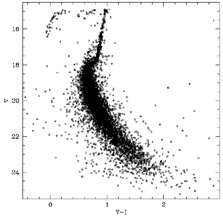
The CMD derived from ground-based data (feb. 02) is shown in Fig. 4. The diagram extends from the upper part of the RGB down to about $V\sim 24$. A reasonably large magnitude range on the MS is crucial in order to report the HST magnitudes (both VEGAMAG and STMAG) to the ground NTT system. The CMD from the dec. 99 run has been obtained under relatively poor seeing conditions and hence came out to be not suited to perform an accurate calibration of the HST data to the ground system. For this reason we adopted the feb. 02 data-set after checking that the two sets of measurements were self-consistent. Fig.5 shows the results of the check.

Figure 4: Ground CMD.

Figure 5: Run to run scatter in the ground measurements.

Figure 6: CMD from HST data.

Figure 7: Final CMD.

5.2 The HST CMD

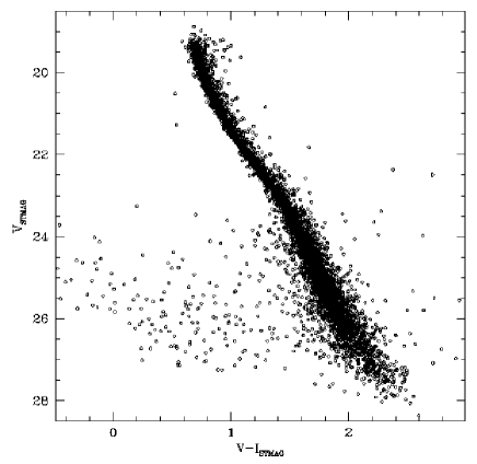
The HST measurements have been averaged, recording also information on the number of frames in which each object was detected in each filter. As final catalog we consider all the stars appearing in at least 80% of the frames (at least 5 V and 7 I). This choice is a good compromise between taking all the measurements and taking only the stars detected in all the frames. The first choice would contaminate the CMD with all the spurious detection that appear by chance on only one frame. The second leads to missing faint objects, like WDs. We remark the fact that the brighter part of the catalog (down to $\mathrm{V}\sim 26.5$) is not altered by this selection criterion, as expected. The HST CMD is reported in Fig. 6, where we show only the VEGAMAG magnitudes.

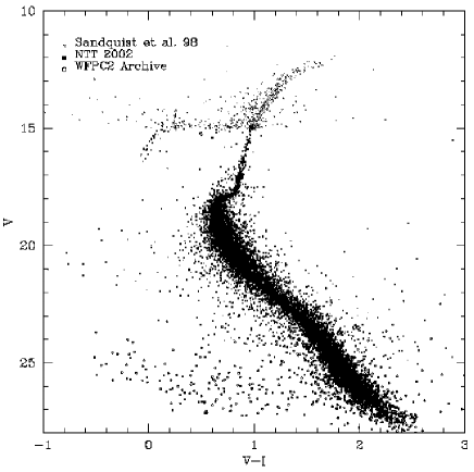
The whole M5 CMD is reported in Fig. 7. The HST data-set extends approximately from $\mathrm{V}=19.5$ to $\mathrm{V}=28$, but the top of the sequence is spread over because the chip is close to the saturation and will not be considered in the following analysis. F555W and F814W magnitudes have been reported to the ground based CMD via a relative calibration equation of the form (for the V magnitude, but it applies to the I magnitudes as well)

$$V_{ground}=V_{HST}+zp+ct\times(V_{ground}-I_{ground})$$

The output for the V magnitude turned out to be identical for STMAG as well as for VEGAMAG, while for the I filter we derived, as expected, different transformations. The two HST magnitudes systems have been checked for self-consistency after reporting them to the ground NTT system. The two transformed magnitudes still show some residuals that, over a range $20<\mathrm{V}<23$ is $\sim$0.01 mag, with a shape that resembles that of a CMD. This is an indication that the color effects were not completely eliminated with the transformations, probably because of the larger scatter in the ground-based CMD and the relatively small magnitude overlap of the ground- and space-based data. However, even at the fainter magnitudes, the overall difference between the two magnitudes is always below 0.05 mag (at $\mathrm{V}\sim 27.5$). In the following, we will adopt as HST transformed magnitudes the ones coming from VEGAMAG, because this system is closer to the ground Vega system, so that the required transformation is smaller and thus less prone to residual uncertainties.

5.3 Mean Ridge Line

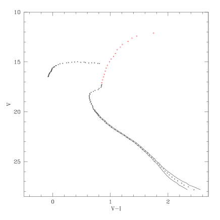
The mean ridge line has been drawn on the faint part by using HST data, on the upper MS until the sub-giant branch with the NTT plus literature data, on the upper part of the RGB and the HB with the (Rosenberg et al., 2000, R00) data, since their RGB is very narrow and well populated. In general, in order to build the ridge line, the CMD has been ’sliced’ in magnitude bins and, for each bin, the median point of the distribution has been determined, together with the associated scatter. Only the objects with the lowest errors have been selected, in order to ensure that the uncertainty on the ridge be small. The zones with a strong curvature, i.e. at the bottom of the SGB, were treated differently, by applying a polynomial fit to that range and projecting the stars along the curved abscissa, then re-fitting iteratively the polynom. In this way, the CMD is sliced along the curve and it is possible to find the median point with high accuracy also in the most bent magnitude bins. Fig. 9 shows the ridge line of the lower MS with its uncertainty strip. The narrowness of the uncertainty strip will be used later to constraint the fit to the subdwarfs sequence. As a comparison term, Fig. 8 shows the ridge line determined as described above, the fiducial by S96 and the ones derived with the same method by using the data of Johnston and Bolte (1998) and R00, that are in close agreement with ours. The irregularities in the

Figure 8: Comparison of ridge lines for M5.

ridge lines obtained with literature data, that can be seen at the base of the RGB, are due to the small size of the magnitude bins chosen to draw the fiducial. Since we are not interested in a careful analysis of those ridge lines, but only show them for sake of comparison, we did not apply any smoothing or more refined technique in order to improve it. It is, however, worth noting that our fiducial line extends about 5 magnitudes below previous works. This fact is crucial because, at least in principle, allows us to check model predictions down to the bottom of the MS, as well as to use very faint subdwarfs to constrain the distance fitting, if any (see below).

Figure 9: The ridge line of the lower MS of M 5 with its uncertainty strip.

Figure 10: Map of the fields covered by this work and recent literature.

Figure 11: Comparison with the data-set of S96

Figure 12: Comparison with the data-set of R00

5.4 Comparison with previous photometry

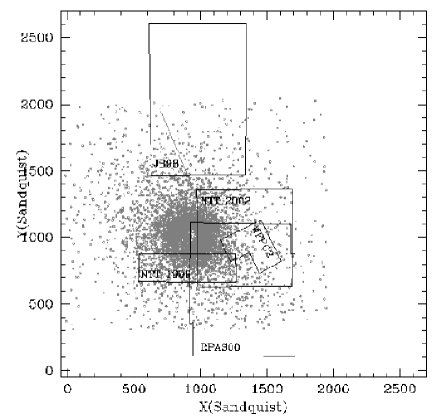
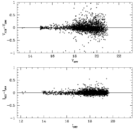
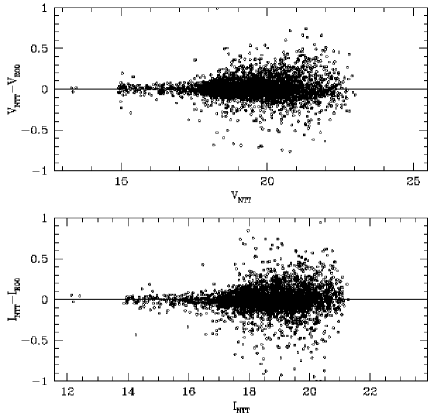
Beside the comparison of the ridge lines, a further check has been done by comparing the NTT CMD with recent literature results, namely R00, Johnston and Bolte (1998) and S96. Fig. 10 shows the positioning of fields observed by us, the HST pointing, and the three comparison works. The plots in Figs. 11 and 12 show the comparison between our magnitudes and the cited ones, where an overlapping of the fields permitted a direct match of the objects. Our data show substantially a good agreement with S96 and R00 but there are a few issues that should be discussed: i) the average scatter is quite large, meaning that a trend with the position could be present. Actually, there is a small residual trend with position, with amplitude of the order of 0.02 mag. In the comparison with the two literature photometries cited above the trend goes toward opposite directions, in the sense that the trend along the X-coordinate, in the reference system of S96, resembles the trend along the Y-coordinate in the R00 data-set, always in the reference system of S96 (all the data have been reported to the system of S96), and viceversa. The amplitude of the trend is larger with S96 than with R00, and is absent if we compare the NTT 1999 data with both S96 and R00. The only valid explanation for this is that a residual flat-field is still present in some data-sets with respect to the others. In fact, in the reduction of the Feb. 2002 data-set, we applied a more refined technique for flat-fielding the data, described in Hainaut (1998), which takes into account also the lowest spatial frenquencies. The 1999 data-set has not been corrected for this effect. On the average, this removed a residual trend in the fluxes. Since this procedure has been applied with success in other works (Monelli et al. 2004, in preparation), we find no reason to discard the procedure or re-calibrate our data in the system of S96 or R00. However, the effect is visible especially at fainter magnitudes ($\mathrm{V}>19$), while is almost absent on the RGB.

Figure 13: Color-metallicity relation for the V-I color, taken from the models of Straniero et al. (1997).

6 Distance via subdwarfs fitting

6.1 Error sources

Before proceeding with the DM fitting, it is appropriate to discuss the contribution of the various error sources to the total uncertainty on the DM. Gratton et al. (2003) report in their Table 1 a detailed list of all the error budget contributors before and after the re-analysis done in that paper. Taking that as a guideline, we can now see how the various uncertainties combine in our case. In Sect. 4 we have already mentioned some of the typical uncertainties in the subdwarfs analysis, and the fact that, since our sample have been drawn from the same lists published by Gratton et al. (1997); Carretta et al. (2000); Reid (1997) and, partially, Gratton et al. (2003), we expect that the uncertainty given by the Lutz-Kelker effect, the Malmquist bias and, clearly, the parallax, are essentially the same. Hence we adopt the values given in Table 1 of Gratton et al. (2003).

Photometric errors are very small both for the subdwarfs (see Table 2) and the cluster ridge line. For this last, in particular, the very precise HST photometry coupled with a good ground-based calibration allowed us to obtain an average error on the ridge line of the order of 0.005 mag at $(\mathrm{V-I})=0.7$. The error from the calibration relation is also very small and of the order of 0.02 mag, since the photometric conditions of the calibration night were close to excellent. In any case subdwarfs and cluster have been observed in the most homogeneous possible conditions and thus, the errors on the photometric calibration are expected to be very small. A residual systematic trend could be present if the calibrated magnitudes were not reported to the standard system, but the obtained values are compliant with all the existing results, and thus we discard this possibility.

Three other sources of error have to be now examined: the metallicity scale, the cluster’s reddening, the presence of binaries. Their contribution affects both random and systematic error.

6.1.1 Metallicity

The metallicity scale is a major issue and has been widely investigated in previous works (see e.g. Gratton et al., 2003; Carretta et al., 2000; Reid, 1997; Pont et al., 1998). There are two main aspects to take into account: i) the spread in metallicity given by the distribution in [Fe/H] of field stars; ii) the relative metallicity scale used. In order to reduce the first effect, the usual procedure is to apply a relation that transforms tha values to a common metallicity (the cluster’s). In our case we decided to use only stars having metallicity values as close as possible to M 5, so that the transformation to a common metallicity is small. In order to estimate it, we used the relation between $\mathrm{[Fe/H]}$ and $\mathrm{(V-I)}$ at $\mathrm{M}_{V}=+6$, taken from the models of Straniero et al. (1997), that is shown in Fig. 13 . A third order polynomial has been found to fit adequately the $(\mathrm{V-I})$ vs $\mathrm{[Fe/H]}$) relation in the range $-2.3<\mathrm{[Fe/H]}<-0.5$. The second effect stands on the systematic difference between the two most commonly used scales, the ZW and the CG. Gratton et al. (1997) use an homogeneous metallicity system, but our subdwarfs sample has been taken from that work and from Reid (1997), who used the ZW scale. Since our cluster has metallicity estimates $\mathrm{[Fe/H]}=-1.1$ in the CG scale, and $\mathrm{[Fe/H]}=-1.4$ in the ZW scale, we found it appropriate to report Reid (1997) values to Gratton et al. (1997), i.e. from ZW to CG, and then selecting stars from the Reid (1997) sample with the reported metallicity close to the cluster’s one.

It should be noted that some of the stars in the present sample have not been recalibrated by Gratton et al. (2003), hence a residual systematic spread might be present which affects the DM fitting as well, due to the co-existence of two slightly different recalibrations. If the value of 0.13 dex is taken as average recalibration offset, we estimate a residual systematic error due to metallicity of $\pm 0.008$ (at 1 $\sigma$) in the $(\mathrm{V-I})$. Given the slope of the MS between $\mathrm{M_{V}}=+5$ and $\mathrm{M_{V}}=+6$, this propagates into an uncertainty of $0.04$ mag. The uncertainity on the metallicity (usually 0.1 dex) is, instead, added to the random error budget, and corresponds, following Gratton et al. (2003), to $\pm 0.08$ mag.

6.1.2 Reddening

The cluster’s reddening also plays a double rôle, since the associated error affects the global random error and the uncertainty on the absolute amount of reddening is a source of systematic error. We shall discuss quantitatively this point below when we present the fitting procedure.

6.1.3 Binaries

The presence of binary stars affects both the subdwarfs and the cluster sample. Although we selected bona fide single stars, a residual quantity of binaries could still affect the subdwarf sample. We rely always on the fact that the sample has been selected from the published lists of Gratton et al. (1997) and Reid (1997), and thus assume their figure for the contribution of subdwarf binaries to the total error, i.e. $\pm 0.02$ (see Gratton et al., 2003). The effect of binaries on the cluster ridge line is slightly more complicated. The effect of the presence of binaries in the cluster is to spread the main sequence toward redder colors and, in extreme cases, to draw a separate sequence, as has been detected in some open clusters (see, e.g., Marconi et al., 1997). In our case, the HST main sequence is very narrow, and a well defined clear binary sequence would be visible. Since this is not the case, we tried to estimate the effect of a MS spread due to an unresolved sequence of binaries. In order to do this, we “rectified” the main sequence and built a color histogram of the brightest portion of the HST MS, that has a uniform width all over the considered range $(20<\mathrm{V}<22)$. A gaussian profile has been fit to this profile, considering only the blue tail of the distribution, that is in principle unaffected by the presence of binaries. The fitted profile has then been subtracted from the original distribution. The residual red tail is an indication of the binary contribution. This procedure is quite robust and gives reliable figures for the uncertainties on the position of the MS locus in the CMD. From this, we derive an estimate of a possible systematic deviation of the MS ridge line from the “true” single star MS given by binaries of $\sigma(\mathrm{V-I})=0.005$, in addition to the random error due to the calculated spread of the MS. Again, this value in color propagates into a $\pm 0.025$ mag of systematic uncertainty. Table 4 below summarizes all the error sources involved in the DM fitting process.

Table 4: Contribution to the total uncertainty, in magnitudes, of the various error sources. Values are at 1$\sigma$ level.

	Field Stars	Cluster
Photometry	$\pm 0.001$	$\pm 0.005$
Calibration	$\pm 0.02$	$\pm 0.02$
Lutz-Kelker	$\pm 0.02$	$-$
Malmquist	Negligible	$-$
Parallax	$\pm 0.01$	$-$
Metallicity (rand.)	$\pm 0.08$	$\pm 0.08$
Metallicity (syst.)	$\pm 0.04$	$\pm 0.04$
Reddening (rand.)	Negligible	$\pm 0.025$
Reddening (syst.)	Negligible	$\pm 0.03$
Binaries	$\pm 0.02$	$\pm 0.025$

6.2 Distance Modulus Fit

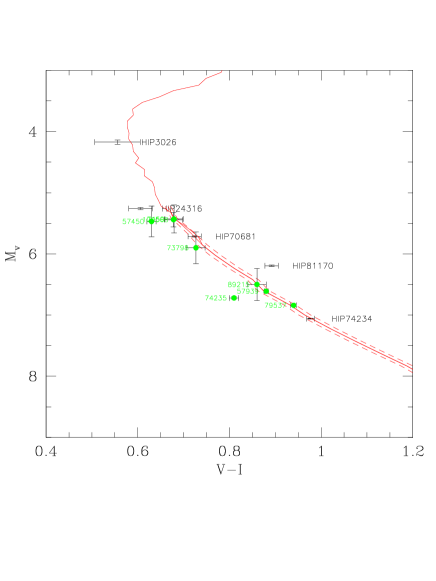
By taking into account all the considerations and the caveats described above, we used the subdwarfs sample to fit a DM to the cluster data. In order to do this, we adopt a value of reddening of $\mathrm{E(B-V)}=0.035(\pm 0.005)$ (Carretta et al., 2000, and refs. therein), corresponding to $\mathrm{E(V-I)}=0.056$, [obtained from the relation in Rieke and Lebofsky (1985): $\mathrm{E(V-I)=1.6\times E(B-V)}$]. The quoted uncertainty has been taken from the literature, and propagates into a $0.025$ uncertainty in magnitude. The DIRBE maps (Schlegel et al., 1998) report a reddening value in the direction of M 5 of $\mathrm{E(B-V)}=0.036$, consistent with the absolute value given in Carretta et al. (2000). As shown in Fig. 14, the brightest calibrating subdwarfs (HIP3026 and HIP24316) turn out to be too blue to fit directly the cluster ridge line, because the cluster MS has already evolved toward the turn-off point. However, they are useful to draw the subdwarfs main sequence locus to be compared with our data. Of the other three stars, HIP81170 is known to be a spectroscopic binary, and this might justify its redder color. The other two, HIP70681 and HIP74234, have the smallest error and have then been used to fit the cluster ridge line. We fit the cluster fiducial line to the subdwarf sequence by shifting the fiducial according to the reddening (in (V$-$I)!) and extiction -$3.1\times\mathrm{E(B-V)}$-, then with a least square fitting of the difference between the used subdwarfs and the cluster fiducial, with their errors. Fig. 14 shows the results of the best fit, that turns out to be $\mu_{0}=14.44$. If a value of $\mathrm{E(B-V)}=0.03$ is adopted, which corresponds to $\mathrm{E(V-I)}=0.048$, $\mu_{0}=14.41$ is obtained. The error on the fit obtained from the combination of the random error sources only is, in both cases, $\pm 0.09$, the uncertainty in the metallicity being the strongest contributor. In order to increase the number of subdwarfs suitable to form a fiducial reference sequence, we added to our sample other subdwarfs listed in Gratton et al. (1997) and Reid et al. (2001), having $\mathrm{[Fe/H]}$ similar to that of M 5 and discarding known double stars. The added stars are listed in Table 3 and shown with different symbols (filled circles) in Fig. 14. It can be seen that most of the added stars draw a good reference main sequence, with the exception of HIP57450 and HIP74235, which are considerably bluer. On the $(\mathrm{V},\mathrm{B-V})$ CMD, however, they lie on the MS, and thus we are inclined to interpret their bluer colors as uncertainties in the I magnitudes, that has been taken from the original HIPPARCOS catalog. For this reason, the two outlying stars have been excluded from the fit.

It can be seen that the added stars define three well separated sequences corresponding to the three metallicity ranges selected, from the lowest (triangles, bluest), to the intermediate (circles), to the highest (squares, reddest).

With the extended sample of subdwarfs, our best estimate for the (dereddened) DM is $\mu_{0}=14.44$ if $\mathrm{E(B-V)}=0.035$ is adopted. If, instead, $\mathrm{E(B-V)}=0.03$ is adopted, as reported in Gratton et al. (1997), the DM turns out to be $\mu_{0}=14.41$, thus confirming the value obtained with the original, and homogeneous, sample.

The error associated to the fit above has been estimated from all the error sources discussed above and reported in Table 4, and considering random and systematic errors separately. From a statistical error propagation all over the involved quantites, the uncertainty associated to the fit turns out to be $\pm 0.09$ mag. A systematic uncertainty, combined from reddening and metallicity scale, of $\pm 0.07$ mag must then be added. The global uncertainty is slightly larger than the one reported by Gratton et al. (2003), probably because the $\mathrm{V-I}$ color is more sensitive to metallicity variation and thus the effect of variation in [Fe/H] and E(B$-$V) are amplified with respect to the B-V color.

Figure 14: Fit of the cluster fiducial to the subdwarfs sequence. The stars with the label on the right belong to the observed sample. The others have been taken from published works.

7 Discussion and Conclusions

This study was aimed at estimating the DM of M 5 through the main-sequence fitting method, using as calibrating sequence a set of local subdwarfs for which the trigonometric parallax from HIPPARCOS was known. In order to achieve our goal we used the same setup telescope+instrument+filters both for the cluster and subdwarfs data, namely the ESO-NTT equipped with the camera SUSI2 and standards ESO V and I filters.

Later, a set of subdwarfs from literature has been added to the original sample in order to improve the sample size, and hence increase the accuracy of the fitting. All the comparisons with recent data from literature show that our data are fully consistent with previous determinations, whose accuracy is known, both for the cluster and the local subdwarfs. A final sample of $\sim$10 subdwarfs has been used to fit a DM to the cluster. By taking into account the two most commonly accepted values for the reddening (i.e. E(B$-$V)=0.03 and 0.035), we obtained two very close values for the (dereddened) DM: $\mu_{0}=14.41\pm 0.09\pm 0.07$ and $\mu_{0}=14.44\pm 0.09\pm 0.07$, respectively, where the first number comes from random error sources, the second from systematic error sources. These values are in good agreement both with Reid (1997) ($\mu_{0}=14.45$ obtained with the subdwarfs having the smallest error on the parallax) and Carretta et al. (2000) ($\mu_{V}=14.59$ corresponding to $\mu_{0}=14.48$), with a slight preference for the shorter value. Vandenberg et al. (2002), instead, found $\mu_{0}=14.38$ with the use of non-diffusive isochrones and $\mu_{0}=14.30$ with diffusive isochrones. In their work, they use a reddening value $\mathrm{E(B-V)}=0.038$ and a metallicity [Fe/H] $=-1.4$ for the cluster, discussing their preference for the ZW scale over the CG on the argument that the metallicity for M 5 is inconsistent with the metal determination for the field stars, if the value is as high as $-$1.1. Moreover, Vandenberg et al. (2002) choose to not report the field stars to a common metallicity, but this effect acts on the spread of the relation rather than on the absolute value.

In order to try to obtain a further constraint on the DM, we tried to use a set of extreme subdwarfs, using an analogous approach to Reid and Gizis (1998), that has been found to be unapplicable because both the main sequence locus at the faint magnitude level of the extreme subdwarfs ($\mathrm{M}_{V}\sim 10$) is dispersed and the subdwarfs of intermediate metallicity define a sequence dispersed as well. In order to reduce the uncertainty, it would have been desirable to have a set of subdwarfs of fainter magnitudes (i.e. below $\mathrm{M}_{V}\sim 7$) to take full advantage of the narrowness of the HST main sequence, but they lack in the HIPPARCOS sample. Moreover, at such faint magnitude level, the lower main sequence stars are very cool and the determination of their metallicity much more uncertain because it is very difficult to take into account all the molecular species in the athmosphere at these low temperatures.