Addendum to “Superimposed Oscillations in the WMAP Data?”

Abstract

We elaborate further on the possibility that the inflationary primordial power spectrum contains superimposed oscillations. We study various effects which could influence the calculation of the multipole moments in this case. We also present the theoretical predictions for two other cosmological observables, the matter power spectrum and the $\mathrm{EE}$ polarization channel.

I Introduction

The possibility that the multipole moments $C_{\ell}$ characterizing the angular distribution of the Cosmic Microwave Background Radiation (CMB) anisotropy on the celestial sphere possess superimposed oscillations has recently been investigated in Ref. [1]. In that article, the superimposed oscillations originate from trans-Planckian wiggles [2] in the primordial inflationary power spectrum but the study of Ref. [1] was meant to be as independent as possible from the details of the underlying model. The presence of oscillations in the primordial spectrum has also been envisaged in Refs. [3]. Then, it has been demonstrated that the superimposed oscillations can cause a significant improvement of the fit to the first year Wilkinson Microwave Anisotropy Probe (WMAP) data [4], thanks to the presence of the cosmic variance outliers around the first Doppler peak. Moreover, it has also been shown that the corresponding drop in the $\chi^{2}$ is statistically significant according to the so called $F$ test. We have since received various inquiries about different effects that could modify the result obtained in Ref. [1] like the influence of the splinning, the consideration of the lensing [5] and the way of estimating the statistical significance of the drop in the $\chi^{2}$. In this addendum, we clarify these issues and, in addition, present new results which are important for the completeness of Ref. [1], namely a fit with an improved $\chi^{2}$ which does not suffer from the back reaction problem and the prediction for two other cosmological observables, the matter power spectrum and the $\mathrm{EE}$ polarization channel. Finally, we would like to emphasize that the general questions analyzed in this Brief Report are important irrespective of the data set used to study them. Therefore, although we use the first year WMAP data, the conclusions reached in this addendum are also valid for the future CMB data releases.

II Robustness of the Wiggles

In this section, we investigate effects that could possibly influence either the numerical calculation of the CMB multipole moments or the statistical analysis of the significance of the “wiggles”.

II.1 Multipoles splinning

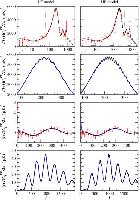
In the case where oscillations are present in the initial power spectrum, a correct numerical computation of the CMB multipole moments requires one to significantly boost the numerical accuracy of the code used to derive the so-called transfer functions [6]. Indeed, it is necessary to know these functions with a high precision if one wants to correctly transfer the contribution of the primordial oscillating spectrum into each multipole moments. In Ref. [1], such high accuracy computations have been performed with the CAMB code [7] and various tests have been carried out in order to ensure that the multipole moments were properly computed. However, one must also pay attention to the sampling and the splinning performed on the multipole moments. They are both present by default to avoid prohibitive computation time. The sampling requires the computation of some multipole moments only and is scale dependent (i.e. $\ell$-dependent) while the splinning interpolates between those multipole moments and thus allows to recover the complete angular spectrum. In Ref. [1], the sampling and splinning have been kept to their default option which is clearly not very appropriate to the case where superimposed oscillations are present. Indeed, as long as the multipole moments $C_{\ell}$ are not computed for each $\ell$, there is the danger to undersample the signal which could result in the appearance of oscillations with an incorrect frequency. At large scales, the multipole moments are always calculated for each value of $\ell$ and at very small scales, the sampling has no effect since the oscillations considered in Ref. [1] are logarithmic in the Fourier space. Therefore, the danger is particularly present at intermediate scales, i.e. around the first Doppler peak. In this Brief Report, we have removed the sampling and the splinning from the CAMB code such that each multipole is now computed. One finds that this does not affect the determination of the multipole moments as long as $\sigma_{{}_{0}}\gtrsim 4\times 10^{-4}$ (with $\varepsilon_{{}_{1}}\simeq 10^{-2}$), but starts to modify the $C_{\ell}$’s at intermediate scales for smaller values in accordance with the previous discussion (see Fig 1). Let us also recall that $\sigma_{{}_{0}}$ is the dimensionless parameter controlling the frequency of the oscillations. It is given by the ratio of the Hubble parameter during inflation to the scale at which the new physics is supposed to show up, $\sigma_{{}_{0}}\equiv H/M_{\mathrm{c}}$. Therefore, we conclude that the sampling or splinning option has an important effect and must be treated with great care. However, despite the above discussion, we show below that we essentially recover the same fit as the one displayed in Ref. [1] up to some small differences.

II.2 Lensing

It has been suggested that CMB lensing effects could blur superimposed oscillations. This could have an influence on the fit found in Ref. [1] since this one corresponds to high frequency wiggles. However, we have checked by mean of the full sky lensing routines implemented in CAMB  [7] that, even in this case, the wiggles around the first Doppler peak remain almost unchanged. This result is expected since the damping due to lensing is mainly proportional to the amplitude of the superimposed oscillations [6]. Moreover, one has to keep in mind that oscillations do not correspond to a localized feature in the Fourier space as studied in Ref. [6], but, on the contrary, constitute a modification which, in some sense, is spread everywhere.

Figure 1: The $\mathrm{TT}$, $\mathrm{TE}$ and $\mathrm{EE}$ angular power spectra for the low frequency (LF) and high frequency (HF) models. A zoom of the $C_{\ell}^{{\scriptscriptstyle{\mathrm{T}\mathrm{T}}}}$’s in the first Doppler peak region is also shown (black curve) and compared with the standard slow-roll prediction (blue curve) calculated the with same cosmological parameters.

II.3 Exploring the “fast” parameter space

We now turn to the effects that could influence the search of the likelihood maxima and/or the analysis of their statistical significance.

As noticed in Ref. [1], the fact that it is necessary to boost the computation accuracy in order to correctly transfer the oscillations significantly increases the computation time for one model. The use of the sampling (see the discussion above), as in Ref. [1], permits us to explore the full (9-dimensional) parameter space using Monte Carlo methods implemented in the COSMOMC code [8]. Nevertheless, this exploration remains clearly limited and may have very well missed the global maximum of the likelihood function. As a consequence, the fit found in Ref. [1] should rather been called “a better fit” than “the best fit”.

In the approach advocated here, where the sampling and splinning have been removed, the situation becomes even worst. In this case, an exploration of the full parameter space, even limited, is no longer possible. In order to tackle this problem, we have fixed the cosmological parameters to their “standard values”, determined from the best fit obtained with a vanilla slow-roll power spectrum. Then, the parameter space to be explored becomes much smaller and now consists in the so-called “fast parameters” only, i.e. the slow-roll parameters, the frequency and the amplitude of the oscillations. This method allows to compute the CMB transfer functions only once and, as a consequence, decreases significantly the computation time of each Markov chain. But, clearly, one should keep in mind that, if the actual best fit is somewhere else in the parameter space, this method will miss it.

II.4 Comparing the fits

In Ref. [1], the “best fit” obtained after a limited exploration of the full parameter space and characterized by $\chi^{2}\simeq 1415.4\,(1340\,\mathrm{DOF})$ has been compared to the best inflationary fit published in Ref. [4], the $\chi^{2}$ of which is given by $\chi^{2}\simeq 1431\,(1342\,\mathrm{DOF})$. Hence the number $\Delta\chi^{2}\simeq 15$ reported in that article. However, the best fit of Ref. [4] has been derived under the assumption that the primordial power spectrum is of the form $k^{n_{{}_{\mathrm{S}}}-1}$ which is not exactly the slow-roll prediction [9]. In addition, no gravitational waves have been included whereas this is automatic in the slow-roll approach because of the consistency check of inflation. Therefore, the number $\Delta\chi^{2}\simeq 15$ does not describe the effect of the wiggles only. In order to disentangle the influence of the wiggles from the effects of the other parameters, one should first determine the best fit obtained with a standard slow-roll power spectrum and then compare this fit to the one obtained after the addition of the oscillations, keeping the same values for the cosmological parameters. Our best slow-roll fit (without the oscillations) corresponds to a model with $\chi^{2}\simeq 1429.3\,(1342\,\mathrm{DOF})$, i.e. a difference of $\Delta\chi^{2}\simeq 2$ in comparison with the best fit of Ref. [4]. Therefore, the effect of adding oscillations is more accurately described by $\Delta\chi^{2}\simeq 13$ rather than $15$. In the following, the evaluation of $\Delta\chi^{2}$ will always refer to a comparison with this slow-roll fit.

Figure 2: Cumulative residual $\chi^{2}$ for the LF and HF models, compared to the standard slow-roll one. The dashed red curve represents the temperature contribution, the dotted blue curve the polarization contribution and the black curve is the sum of these two effects.

II.5 The new improved fits

Type	$|x|\sigma_{{}_{0}}$	$\sigma_{{}_{0}}$	$h$	$\Omega_{\mathrm{b}}h^{2}$	$\Omega_{\mathrm{dm}}h^{2}$	$\Omega_{\Lambda}$	$\tau$	$P_{\mathrm{scalar}}$	$\epsilon_{{}_{1}}$	$\epsilon_{{}_{2}}$	$n_{\mathrm{s}}\equiv 1-2\epsilon_{{}_{1}}-\epsilon_{{}_{2}}$	$\chi^{2}/\mathrm{DOF}$
HF	$0.107$	$1.7\times 10^{-4}$	$0.734$	$0.024$	$0.116$	$0.74$	$0.1294$	$23.6\times 10^{-10}$	$0.012$	$-0.0298$	$1.005$	$1418.4/1340$
LF	$0.047$	$3.4\times 10^{-4}$	$0.734$	$0.024$	$0.116$	$0.74$	$0.1294$	$23.7\times 10^{-10}$	$0.010$	$-0.0226$	$1.002$	$1420.8/1340$

Table 1: Best HF and LF fit parameters from the WMAP data. The pivot scale and the time $\eta_{{}_{0}}$ (see Ref. [1]) are still chosen such that $k_{*}/a_{{}_{0}}=M_{\mathrm{c}}=0.01\,\mathrm{Mpc}^{-1}$.

In this section, we present two interesting models corresponding to two local maxima of the likelihood, the improvements discussed before having been taken into account. The results are summarized in Table 1. One model, labeled “HF” (high frequency), corresponds to very rapid oscillations, while the other, labeled “LF” (low frequency), has a smaller frequency. The HF model is essentially similar to the “best fit” model found in Ref. [1] (see the Table I in that article), hence justifying the claim that one recovers almost the same solution despite the new effects studied in this addendum. The improvement of the $\chi^{2}$ is now $\Delta\chi^{2}\simeq 11$ with two additional parameters, that is to say slightly less good ($\Delta\chi^{2}\simeq 2$) but still of the same order of magnitude as the fit found in Ref. [1]. The corresponding $F$ probability is $F_{\mathrm{proba}}\simeq 0.6\%$ and hence the improvement remains statistically significant. As discussed in Ref. [1], this model suffers from a severe back-reaction problem.

As already mentioned, the LF model seems to be also favored by the data. Admittedly, the improvement of the $\chi^{2}$ is less good with $\Delta\chi^{2}\simeq 8.5$ for two additional parameters but corresponds to $F_{\mathrm{proba}}\simeq 1.87\%$, demonstrating that it is also statistically significant. Furthermore, this model no longer suffers from the back reaction problem which is, from the theoretical point of view, an important advantage. Indeed, as can be seen from Eq. (11) in Ref. [1], back reaction effects are important for small values of $\sigma_{{}_{0}}$, i.e. in the case of high frequency wiggles. This explains why the LF fit can satisfy the back reaction constraint.

Finally, in Fig. 1, we present the HF and LF fits and in Fig. 2 we plot the cumulative residual $\chi^{2}$ with respect to the standard slow-roll model.

III Other cosmological observables

In Ref. [1], we have only presented predictions for the quantities $C_{\ell}^{{\scriptscriptstyle{\mathrm{T}\mathrm{T}}}}$ and $C_{\ell}^{{\scriptscriptstyle{\mathrm{T}\mathrm{E}}}}$. However, two other important observables, for which data already exist or will be available very soon, are the matter power spectrum and the $\mathrm{EE}$ polarization channel, $C_{\ell}^{{\scriptscriptstyle{\mathrm{E}\mathrm{E}}}}$. In this addendum, we calculate these two observables in the case where superimposed oscillations are present.

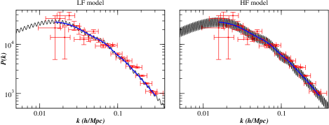
In Fig. 3, we present the matter power spectrum corresponding to the two HF and LF best fit values given in Table 1, together with the current SDSS [10] deconvolved power spectra in the linear regime. It is obvious that the oscillations are transfered from the initial power spectrum to the matter power spectrum since there are linked by a transfer function only, $P(k)=T(k)P_{\rm\zeta}$. For the HF and LF fits, we see that the oscillations are well within the error bars. We have also computed the convolution of the LF and HF oscillatory power spectra with the sloan survey windows functions (the blue curves in Fig. 3). It is clear that the HF and LF convolved matter power spectra are fully degenerate with the vanilla slow-roll power spectrum. As a consequence, we conclude that, with the currently available large scale structure data, no constraint can be put on the parameters controlling the shape of the oscillations.

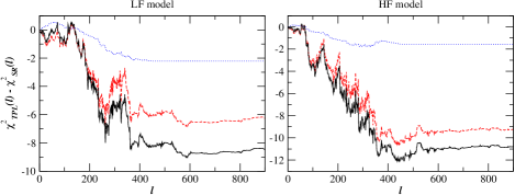
Finally, in Fig. 1, we present the $\mathrm{EE}$ polarization multipole moments. As can be seen from the figure, the oscillations are also transfered to $C_{\ell}^{{\scriptscriptstyle{\mathrm{E}\mathrm{E}}}}$. It is likely that the future polarization measurements will play an important role in deciding whether the superimposed oscillations are really present in the data since the drop in the $\chi^{2}$ is, for the moment, almost insensitive to polarization (see Fig. 2). With more accurate polarization data at our disposal, this situation will certainly change.

Figure 3: Predicted matter power spectra for the LF and HF models (black curve), compared to the deconvolved SDSS data [10]. The convolved power spectra by the sloan survey windows function (blue curve) are also plotted.

IV Conclusions

In this addendum, we have investigated various effects that could influence the presence of wiggles in the CMB multipole moments. We have shown that the splinning is an important parameter which, in the presence of high frequency superimposed oscillations, can influence the shape of the of CMB angular spectrum at intermediate scales. We have shown that the model presented in Ref. [1] remains favored by the data (up to a variation of $\Delta\chi^{2}\simeq 2$). Two other cosmological observables have also been presented, namely the matter power spectrum and the $\mathrm{EE}$ polarization multipole moments. With the available data, we have concluded that these two observables do not affect the results reached in Ref. [1].

A last remark is in order here. In Ref. [1], the statistical significance of the wiggles has been discussed by means of the $F$ test. This was motivated by the fact that the $F$ test only requires the knowledge of the likelihood maxima for the different models under consideration. However, by only varying the “fast parameters”, one may expect to efficiently probe the corresponding subspace. Therefore, an interesting improvement of the present work would be to compute the statistical evidence in this subspace, thus providing us with a different test of the statistical significance of the wiggles.