Testing for Non-Gaussianity in the Wilkinson Microwave Anisotropy Probe Data: Minkowski Functionals and the Length of the Skeleton
Abstract
The three Minkowski functionals and the recently defined length of the skeleton are estimated for the co-added first-year Wilkinson Microwave Anisotropy Probe (WMAP) data and compared with 5000 Monte Carlo simulations, based on Gaussian fluctuations with the a-priori best-fit running-index power spectrum and WMAP-like beam and noise properties. Several power spectrum-dependent quantities, such as the number of stationary points, the total length of the skeleton, and a spectral parameter, , are also estimated. While the area and length Minkowski functionals and the length of the skeleton show no evidence for departures from the Gaussian hypothesis, the northern hemisphere genus has a that is large at the 95% level for all scales. For the particular smoothing scale of FWHM it is larger than that found in 99.5% of the simulations. In addition, the WMAP genus for negative thresholds in the northern hemisphere has an amplitude that is larger than in the simulations with a significance of more than . On the smallest angular scales considered, the number of extrema in the WMAP data is high at the level. However, this can probably be attributed to the effect of point sources. Finally, the spectral parameter is high at the 99% level in the northern Galactic hemisphere, while perfectly acceptable in the southern hemisphere. The results provide strong evidence for the presence of both non-Gaussian behavior and an unexpected power asymmetry between the northern and southern hemispheres in the WMAP data.
Subject headings:
cosmic microwave background – cosmology: observations – methods: statistical1. Introduction
Over the last few years much interest has been focused on constraining non-Gaussian contributions to the cosmic microwave background (CMB). This interest is based on three facts: First, if the CMB anisotropy field is in fact Gaussian, the power spectrum (or, equivalently, the two-point correlation function) contains all the statistical information required to characterize the field. Under the Gaussian hypothesis, therefore, one may compress the statistical information content of the full data set, consisting of several millions of data points, into one single vector, , of perhaps a few thousand power spectrum coefficients. Second, most current theories predict a Gaussian (or at least nearly Gaussian) anisotropy field, and significant departures from Gaussianity could point toward new physics (e.g., Wang & Kamionkowski 2000; Lyth & Wands 2002; Bouchet et al. 2002; Bernardeau & Uzan 2003). Finally, residual foregrounds or systematic artifacts caused by the instrument or data processing are likely to manifest themselves as non-Gaussian signal contributions. Tests for non-Gaussianity afford possible methods for detecting, characterizing, and subsequently removing such effects. Further impetus for the study of such signatures has arisen in recent months from putative detections of non-Gaussian features in the Wilkinson Microwave Anisotropy Probe (WMAP; Bennett et al. 2003a) first-year sky maps (Coles et al. 2004; Naselsky et al. 2003; Vielva et al. 2004; Copi, Huterer, & Starkman 2004; Park 2004; Eriksen et al. 2004).
There is no unique way for a random field to manifest non-Gaussianity; hence, there is no generically superior, high-sensitivity test for all of the possible ways in which a field can be non-Gaussian. In order to perform a thorough analysis, one therefore has to apply a wide range of qualitatively different tests that attack the problem from different directions. Different classes of tests, e.g., harmonic space methods such as the bispectrum and trispectrum, the one-point distribution function (e.g., skewness and kurtosis), -point correlation functions in real space, wavelet-based tests, and morphological measures such as those described in this paper, all probe different aspects of deviation from Gaussianity and are probably sensitive to different classes of such behavior. While tests performed in harmonic space are most sensitive to non-Gaussianities concentrated on characteristic angular scales as quantified by , tests performed in real space are most sensitive to non-Gaussianities localized to specific regions on the sky.
In this paper we present estimates of four functions, all related to the morphology of hot and cold areas, computed from the WMAP first-year data. These four functions are the three Minkowski functionals (Minkowski, 1903) and the “skeleton” length (Novikov, Colombi, & Doré 2003), which all are known for their ability to measure non-Gaussian effects. Historically, cosmological tests based on topology were probably introduced by Gott, Melott, & Dickinson (1986) in the context of the distribution of galaxies. The genus Minkowski functional (or equivalently, the Euler-Poincaré characteristic) was first suggested as a way of detecting the non-Gaussianity of the CMB by Coles & Barrow (1987) and Coles (1988). Topological tests of the CMB anisotropies were developed further by, e.g., Gott et al. (1990), and finally, the full set of Minkowski functionals was introduced into the field of CMB research by Schmalzing & Górski (1998), Winitzki & Kosowsky (1998), and Novikov, Feldman, & Shandarin (1999). These have recently been joined by the skeleton length measure (Novikov et al., 2003), which naturally belongs to the same group of statistics. One major advantage of these tests is that they are relatively undemanding on computer resources, and therefore it is feasible to apply these tests to the megapixel CMB data sets from modern experiments, such as WMAP.
While the skeleton length has not been measured for the WMAP first-year data set to this date, at least three other groups have computed the genus Minkowski functional for this data set, namely, Komatsu et al. (2003), Colley & Gott (2003), and Park (2004). While the former group does not describe their algorithms in great depth, the latter two use pixel-by-pixel methods for computing the genus. We choose a third method based on the first and second derivatives of the map for finding all stationary points in the map. Although each of the four functions has an explicit analytic expectation value for a Gaussian field, we find it generally more convenient to calibrate our results with Monte Carlo simulations in order to assess the importance of the effects of realistic beam profiles, non-uniform noise, and partial sky coverage. As a by-product of these functional measurements, we also determine a number of power spectrum-dependent quantities, such as the number of extrema and the total length of the skeleton. Each of these statistics may be regarded as an independent test of the underlying power spectrum.
It should be noted that another recent analysis by Hansen et al. (2004) computes the local curvature distributions of the WMAP data, using a technique very similar to ours. Although they do not obtain quite as strong detections with this curvature measure as determined here with the genus statistic, the two sets of results are in excellent agreement.
The rest of the paper is organized as follows. In §2 we review the definitions of the Minkowski functionals and the skeleton, while §3 describes how to compute each of these functions from a pixelized map. The necessary preparations and the statistical methods to be applied to the actual WMAP data are summarized in §§4 and 5. Finally, the results are shown in §6, before comparing with other results and making some final remarks in §7.
2. The Estimators
In our analysis, we study the normalized anisotropy field,
| (1) |
where the standard deviation of the anisotropy field over the observed region of area is defined by .
This normalization is necessary in order to minimize the impact of the realization-dependent power spectrum – we are more interested in departures from Gaussianity, than in possible power spectrum deviations.
For a study of the geometric properties of the CMB field to be meaningful, we have to consider the shape of connected sets. This is done here, as usual, by studying excursion sets of the two-dimensional CMB-field on the celestial sphere, i.e., the set consisting of the parts of the sky having a temperature above a given threshold . The main interest is in seeing how the morphological descriptors vary as functions of .
2.1. The Minkowski functionals
A well known theorem of integral geometry (Hadwiger, 1957) says that under relatively unrestrictive conditions (that the descriptors are rotationally and translationally invariant and that they preserve additivity and convex continuity), the morphology of a convex body in -dimensional space can be completely described by Minkowski functionals (Minkowski, 1903). Therefore, a morphological description of the CMB anisotropy field on the two-dimensional celestial sphere can be obtained through three Minkowski functionals, and all possible morphological descriptors obeying the above conditions can be expressed as a linear combination of those. Thorough reviews of the two-dimensional Minkowski functionals on a sphere are given by, e.g., Schmalzing & Górski (1998) and Winitzki & Kosowsky (1998).
The first two-dimensional Minkowski functional we use is the normalized area of the excursion set , i.e., the area of as a fraction of the full area of the survey. Using the HEALPix111Available from http://www.eso.org/science/healpix pixelization (Górski, Hivon, & Wandelt 1999), in which all pixels have exactly equal area, the area functional is easily computed by counting the number of pixels with a field value above the threshold under consideration,
| (2) |
The second two-dimensional Minkowski functional is the length of the border of the excursion set,
| (3) |
The details of computing this measure on a pixelized map are provided in detail below. We follow the convention of normalizing the function to have unit integral value,
| (4) |
The third Minkowski functional is the genus , which is defined as the (normalized) number of connected hot spots (regions above the threshold, i.e., connected parts of ) minus the number of connected cold spots (regions below the threshold, i.e., connected parts of the whole survey area minus ). However, here we approximate with the number of maxima plus the number of minima minus the number of saddle points in the excursion set (Novikov, Schmalzing, & Mukhanov 2000), divided by the sum of all stationary points in the whole un-thresholded field,
| (5) |
2.2. The skeleton length
The skeleton length was recently introduced as a diagnostic for Gaussianity by Novikov et al. (2003). For a random field on , it is defined as the zero-contour line of the map
| (6) |
where and denote the first derivatives of the random field in two orthogonal directions and the -values denote the second derivatives.
When applying the above expression to a field on the sphere, it is crucial to notice that is a rotationally invariant quantity. Therefore, we may construct a local coordinate system at each point and compute the derivatives in that local system before adding them together. In particular, we may choose our coordinate system to be the standard latitude-longitude system on the sphere, and the derivatives may be chosen to be the covariant derivatives. The skeleton map on the sphere may therefore be expressed by
| (7) |
where the semicolons as usual denote covariant derivatives. We later discuss how to compute them.
Although Equation (7) may be difficult to interpret, its geometric interpretation is intuitive: the zero-contour lines of are the set of lines that extend from extremum to extremum along lines of maximum or minimum gradient, and the set of all such lines is collectively called the skeleton of the field.
The statistic we are interested in is the length of the skeleton of that part of the field that lies above some threshold , normalized by the length of the skeleton of the whole un-thresholded field. Obviously this can be computed by the same algorithm as is used for computing the length Minkowski functional , since the skeleton is the zero-contour of the -map.
For a Gaussian field (Novikov et al., 2003), the differential skeleton length depends only on one spectral parameter, , defined as
| (8) |
where is the variance of the map, is the variance of the first-order derivatives, and is the variance of the second-order derivatives. We later use this quantity as an independent statistic when studying the WMAP data.
Actually, it has been shown that for a Gaussian field, the differential skeleton length is
| (9) |
3. Algorithms
As seen from the definitions, in addition to just counting pixels for the area Minkowski functional (Equation 2), we need two distinct algorithms for computing the four functions (i.e., the three Minkowski functionals and the length of the skeleton). For the skeleton length and for the length Minkowski functional it is necessary to estimate the length of a contour line, and for the genus functional the positions of all stationary points must be located and the field values at these points estimated.
Both these operations, as well as the determination of the skeleton, depend on derivatives of the field. Such derivatives are well-behaved only if the map itself is smooth (that is, not dominated by pixel noise), and we therefore consider it prudent to filter each map before applying our algorithms. In addition, simple experiments show that robust estimation of the contour line lengths requires a high pixel resolution compared to the smoothing scale: adequate smoothing is then an essential step in the analysis. A brief discussion of this and related topics is given in §4. As pointed out by, e.g., Winitzki & Kosowsky (1998), numerical techniques for estimating the length of a contour line or positions of stationary points on real CMB maps with noise, pixelization, masks, etc., have to be chosen with care. Our experiments show that the algorithms employed here are sufficiently insensitive to such effects and give accurate results.
3.1. Measuring the length of an iso-contour line
Our starting point is thus a smoothed, pixelized map in which we know the field values at the pixel centers. We want to trace the underlying contour lines between those pixel centers and estimate their lengths. The method for doing so is based on linear interpolation and is almost identical to the methods adopted by, e.g., Shandarin et al. (2002) and Novikov, Feldman, & Shandarin (1999). However, we also use this method for locating the stationary points; therefore, we review the algorithm in detail here.
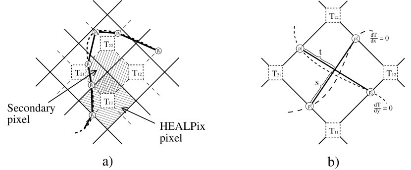
We start by constructing a secondary set of pixels, defined by letting the original pixel centers be at the corners of the new, secondary pixels. The secondary pixels are then checked to determine those that are crossed by a contour line. These are obviously the secondary pixels where at least one vertex has a lower value and at least one vertex has a higher value than the contour line. This process is illustrated in the left-hand panel of Figure 1.
Once such a “crossed” secondary pixel has been found, it is easy to determine through which edges the contour line passes; a contour line crosses an edge if one vertex has a field value larger than the contour value and the other vertex has a smaller value. The point on the edge where the contour line crosses is estimated by a linear approximation,
| (10) |
Here (given as an unnormalized vector from the center of the sphere) is the point at which the contour line crosses the secondary pixel edge, and are the field values at the two vertices with corresponding positions and , while is the field value on the contour line.
After locating both points on the edges of the secondary pixel where the contour line enters and exits the pixel, the angular length of the line segment within that pixel is estimated by computing the dot product of the two vectors,
| (11) |
where are the normalized unit vectors found in Equation (10).
In those cases in which more than two edges of a pixel are crossed by a contour line, we assume that two contour lines cross each other inside the pixel. The justification for this assumption is simply that we are interested only in the total length of the contour line, not its shape, and the possible error introduced in the total length by this assumption is obviously very small because of the small pixel size.
3.2. Locating the stationary points of a random field on a sphere
In order to compute the genus Minkowski functional, we need to locate all stationary points – both minima, maxima, and saddle points. While extrema alone may be found by searching for pixels that have neighbors with all higher or lower temperature values (as is implemented in the HEALPix hotspot facility), this method cannot be used for locating saddle points. Therefore, a different approach is adopted in this work, namely, a method based on the covariant derivatives of the random field.
A stationary point has by definition vanishing first partial derivatives computed in two orthogonal directions. The particular type of stationary point is determined by the eigenvalues of the Hessian matrix: if all eigenvalues are positive, the point is a minimum; if all are negative, the point is a maximum; and if there are both positive and negative eigenvalues, it is a saddle point. To find the positions and types of all stationary points, we therefore need to be able to efficiently compute the first and second derivatives of the temperature field. We use the covariant derivatives in the standard polar coordinate system,
| (12) | ||||
| (13) |
In this paper, these derivatives are only used to determine the skeleton and to locate the stationary points, but, as shown by Schmalzing & Górski (1998), it is possible to express all the Minkowski functionals in terms of the field itself and its first- and second-order derivatives.
It is most convenient not to compute the covariant derivatives of the temperature anisotropy field directly from the pixel values, but rather to do it from the expansion of the anisotropy field in spherical harmonics,
| (14) | ||||
| (15) |
where the partial derivatives are found term by term. Here is a normalization constant.
By using the identity for associated Legendre polynomials,
| (16) |
where , one finds that the covariant derivatives are given by
These derivatives may then be computed very efficiently using the HEALPix routines map2alm and alm2map.
In principle, one could go through this process once more to find equivalent expressions for the second derivatives. However, in practice one obtains numerically more stable results by making new pixelized maps of the first derivatives of the original map, expanding those in spherical harmonics using HEALPix routines, and then applying the above formulae to them, rather than using second-order expressions on the temperature map itself. The cost for this extra stability comes in the form of two extra spherical harmonics transforms, but the extra CPU time required is acceptable. By repeated application of the above formulae we thus find all first and second derivatives of the anisotropy field in all pixel centers.
The next problem is to find the points of intersection of the lines and , since the stationary points must be at these intersections. This is done with an algorithm similar to that described for tracing the iso-contour lines; once again we focus on the set of secondary pixels, but this time we search for secondary pixels being crossed by both “iso-contour lines” and .
Once such a secondary pixel is found where the two zero-derivative curves cross its edges, it must be determined whether the two lines actually cross each other inside that pixel. We find the position of all four edge crossings (two for each contour line) as for Equation (10), project these positions into a local, two-dimensional coordinate system centered on the pixel, and solve the system
| (17) |
of linear equations. Here the four are four two-dimensional vectors representing each of the four crossing-points of the edge of the pixel.
If , the two lines do intersect each other inside the pixel, and the point of intersection is estimated by substituting either or into the respective side of the above equation. Figure 1(b) illustrates this method.
After locating such a stationary point, one must then estimate both the field value (for thresholding) and the second derivatives at that point. For this purpose we adopt a weighting method that takes into account the values at all four vertices. First, the angular distance between the point of intersection and the four vertices is computed,
| (18) |
The relative weights, , are then evaluated as the smallest angular distance divided by ,
| (19) |
Finally, the true weights, , are found by normalizing the sum to unity, .
The field value and the second derivatives at the point of intersection may now be estimated as weighted sums over the vertices,
| (20) | ||||
| (21) |
The last step in this process is to determine the type of stationary point. This is done from the characteristic equation,
| (22) |
The stationary point is a maximum if the solutions of the characteristic equation , a minimum if and a saddle point if and have different signs (assuming that the point is non-degenerate, i.e., that which is always true for real-world fields).
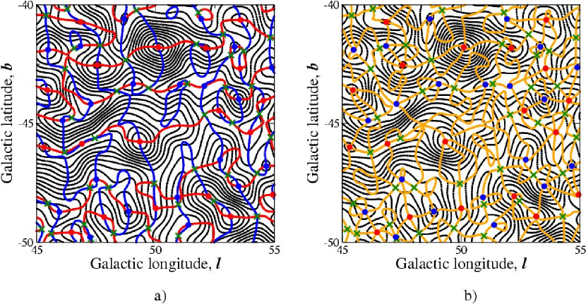
The procedure is illustrated in Figure (2). A contour map of a patch of the CMB sky is shown in the left panel. The contours are the blue lines and the contours are the red lines. The stationary points (maxima: red filled circles; minima: blue filled circles; saddle points: green crosses) are seen to be at the intersections of the blue and red lines. In the right-hand panel the skeleton of the field is overlaid on the same map as a yellow contour line.
4. The WMAP data and the simulations
The aim of this paper is to measure the three Minkowski functionals and the length of the skeleton as a function of the threshold height for the WMAP first-year maps and to compare these to the same quantities estimated from a Monte Carlo set of 5000 simulated Gaussian sky maps. The Monte Carlo ensemble is based on the best-fit WMAP power spectrum with a running index, which may be down-loaded from the LAMBDA222http://lambda.gsfc.nasa.gov Web site.
Our study is based on the co-added WMAP map (Hinshaw et al. 2003), and in order to produce the best possible approximations to this map, the simulations are processed in exactly the same way as the WMAP map. In short, each realization is constructed as a weighted sum over each of the cosmologically important WMAP channels (Q1, Q2, V1, V2, W1, W2, W3, and W4), taking into account the particular beam and noise properties of each channel (Spergel et al., 2003). We use foreground-corrected maps produced by the template fitting method of Bennett et al. (2003b) to suppress foreground contamination.
The publicly-released maps are available at the LAMBDA Web-site. However, a problem was recently discovered with these maps (see the LAMBDA web page333http://lambda.gsfc.nasa.gov/product/map/IMaps_cleaned.cfm, where a more thorough description is given); the templates used in this process were convolved with a too low (the maximum multipole component), resulting in ringing around strong point sources. For this reason we have also generated our own templates and performed the analysis for these maps as well. The differences between the two sets of results are insignificant on the scales we consider; therefore, we choose to report only the results for the official maps in what follows.
For both the WMAP data and the simulated maps, a number of data processing steps are performed to minimize the impact of residual foregrounds, the applied Galaxy cut, pixel noise, etc. First, the WMAP Kp0 mask with point sources included (i.e., we do not exclude the 700 point sources present in the mask specified by the WMAP team) is defined as the base mask. The decision not to exclude the 700 point sources is based on two factors. First, we are mainly interested in scales larger than , and for such large scales the impact of point sources is small (see, e.g., Spergel et al. 2003). Later in the paper the impact of point sources is explicitly tested by applying a median filter to the map. Second, since the maps are smoothed, we also have to expand the mask accordingly. If the 700 point sources actually were excluded by the base mask, the expanded mask would accept only a very small fraction of the sky. It is therefore better to include the point sources in the analysis, and then later on determine from the results themselves whether this is justified or not. To test for any effects of the exact shape of the mask, we also perform our analysis using a base mask with the additional constraint .
The next processing step is to remove the best-fit mono- and dipoles from the maps, with coefficients computed from the accepted region only. Then, the masked region is nullified, and the mask boundary is apodized, before the maps are smoothed with a Gaussian beam of given FWHM (which will be varied, see below). This smoothing operation consists of a spherical harmonics transform of the original map, followed by a multiplication with the Legendre transform of the Gaussian beam. Then the smoothed map is constructed through an inverse spherical harmonics transform. At this point we keep the final multipole expansion components, , for computing the derivatives (see §3) at a later stage.
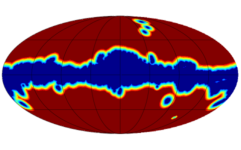
The next step is to expand the excluded regions of the mask in all directions as a safeguard against border effects. This is done according to the procedures of Schmalzing & Górski (1998); the mask map consisting of zeros and ones is convolved with a Gaussian beam of the required FWHM, and the new, expanded mask is then determined by including all pixels with values higher than some given threshold, for instance, 0.95 or 0.99. For maximum safety we perform this operation twice, each time with a limiting threshold of 0.99. The resulting masks are shown in Figure 3. Finally, the map is normalized according to Equation 1, including pixels in the accepted region only.
The analysis is carried out for a large number of smoothing FWHMs in order to probe different angular scales. The beam widths selected were , , , , , , , , , , and FWHM444After having completed the computations, we discovered an error in a computer code that effectively multiplied all smoothing FWHMs by . Thus, the FWHMs that originally had been chosen to be multiples of were in reality multiples of , causing the somewhat unnatural looking smoothing scales in this paper.. Note that this smoothing is applied directly to the observed maps; therefore, the Gaussian smoothing beam is in addition to the experimental WMAP beams. In total, the narrowest of the beams ( FWHM) is sensitive to multipoles up to about ; therefore, both noise and point sources are expected to play a major role at this and smaller scales. Here it is worth noticing that Park (2004) considered even smaller scales, since the maps were not explicitly smoothed at all, except for a small effect introduced by a stereo-graphical projection. However, in the subsequent analysis, the 700 point sources resolved by WMAP were masked out, and it was therefore possible to produce results on smaller scales than presented in this paper.
The maximum multipole component, , in each run is chosen to match the corresponding FWHM. In particular, the values of we choose are 650, 600, 550, and 450 for FWHMs between and and 350 for the larger beams. The HEALPix resolution parameter used internally in the computations is . By increasing from 512 to 1024, the total skeleton length is increased by a few percent for the narrowest beam. However, by increasing from 1024 to 2048, the total skeleton length is increased only by a negligible amount. Thus, is the lowest resolution able to support all our analyses, although lower resolutions could have been chosen individually for the wider beams.
The four statistics are estimated for 200 values of the threshold height between and , but only a subset of these values are used in each of the subsequent analyses. Each statistic is evaluated independently on the northern and southern Galactic hemispheres. Interesting hemisphere effects have been reported by several authors (Eriksen et al. 2004; Park 2004), and we focus our tests accordingly.
5. Quantifying the degree of agreement between simulations and observations
In order to quantify the degree of agreement between the simulations and the observations, we adopt a diagonal statistic of the form
| (23) |
where is the threshold level, is the average of the simulations, and is the standard deviation of the measure under consideration. This statistic is computed for both the simulations and the observed functions, and the fraction of simulations with value lower than the determined from the real WMAP map is connected to the confidence level at which to either accept or reject the null-hypothesis – that the observed field is a natural member of the Gaussian Monte Carlo ensemble.
Note that we choose a diagonal statistic for the functions in this paper. In our experience, the ordinary statistic, which takes into account bin-to-bin correlations through the covariance matrix, behaves rather badly if the functions under study are binned with a narrow bin size, as is the case here. If neighboring bins are strongly correlated, the covariance matrix converges very slowly, and in the study here, 5000 simulations would not be sufficient to produce robust results. Furthermore, when the bin-to-bin correlations are strong, the off-diagonal terms become more and more dominant, and the shape of the inverse covariance matrix resembles that of a Mexican hat. A Mexican hat matrix is the same as a high-pass filter. Therefore, if the bin-to-bin correlations are strong, the covariance matrix statistic is more sensitive to fluctuations in the functionals, rather than absolute deviations. In some cases, one actually finds that the covariance matrix statistic accepts functions that should obviously be rejected by eye.
However, if the proposed model for the simulations is an adequate description of the real data, then no statistic should be able to distinguish between the simulations and the observations. The choice of statistic is therefore only a question of what one wants to measure.
For the genus we adopt the machinery of Park (2004) and perform a parametric fit of the form
| (24) |
where and are free parameters. For a Gaussian field it is expected that , while is a normalization constant depending on the power spectrum. This fit is performed over three different ranges in , namely, , , and . The corresponding amplitudes are named , , and and indicate, respectively, the best-fit total amplitude and negative and positive amplitudes. We also define an asymmetry parameter by
| (25) |
For a Gaussian field there should be no asymmetry in the shape of the genus, and consequently should also be zero. Note that this definition of differs slightly from that of Park (2004).
The fit of to the data is implemented as a non-linear search (using NAG555Numerical Algorithms Group, http://www.nag.co.uk routines), which minimizes the functional
| (26) |
where is a weight factor. In this paper we choose inverse variance weighting, , where is the simulated variance of the particular genus bin. However, almost all results are practically independent of this particular choice, with the notable exception of the total range amplitude for realizations with a large asymmetry parameter . In those cases, one may find that the amplitude depends, but only weakly, on the weighting scheme. Moreover, we are mostly concerned with the negative and positive threshold amplitudes and the asymmetry parameter itself, and these quantities are very robust against different weighting schemes.
6. Results
| FWHM | Length | ||||
|---|---|---|---|---|---|
| Full sky | |||||
| 0.497 (95.2%) | 1870. (84.3%) | 11 258 (98.4%) | 11 330 (99.9%) | 22 565 (99.9%) | |
| 0.505 (93.9%) | 1584. (93.4%) | 8558 (99.5%) | 8515 (96.2%) | 17 049 (99.3%) | |
| 0.503 (93.6%) | 1267. (93.0%) | 5723 (91.8%) | 5701 (81.7%) | 11 422 (92.2%) | |
| 0.478 (93.4%) | 904.6 (67.9%) | 2939 (25.9%) | 3019 (97.5%) | 5958 (80.5%) | |
| 0.468 (93.4%) | 677.8 (58.6%) | 1648 (6.5%) | 1716 (88.9%) | 3352 (32.9%) | |
| 0.465 (93.9%) | 530.1 (84.0%) | 1042 (49.8%) | 1063 (85.9%) | 2100 (71.3%) | |
| 0.470 (95.0%) | 429.7 (97.6%) | 691 (48.2%) | 705 (80.7%) | 1395 (70.0%) | |
| 0.478 (96.4%) | 354.2 (85.7%) | 494 (73.4%) | 499 (84.7%) | 986 (78.7%) | |
| 0.488 (97.2%) | 297.0 (56.0%) | 366 (82.5%) | 348 (28.5%) | 719 (72.0%) | |
| 0.496 (97.7%) | 254.4 (52.0%) | 285 (94.9%) | 264 (35.3%) | 554 (87.7%) | |
| 0.505 (98.0%) | 221.2 (54.1%) | 216 (80.5%) | 204 (34.0%) | 422 (70.1%) | |
| Northern hemisphere | |||||
| 0.535 (98.7%) | 634.5 (70.3%) | 2851 (62.4%) | 2854 (65.9%) | 5694 (60.4%) | |
| 0.517 (98.9%) | 454.8 (60.6%) | 1493 (57.6%) | 1537 (98.6%) | 3023 (91.2%) | |
| 0.511 (98.9%) | 334.0 (23.9%) | 811 (1.3%) | 875 (92.7%) | 1681 (27.2%) | |
| 0.514 (99.0%) | 268.2 (83.6%) | 524 (41.9%) | 545 (90.5%) | 1068 (75.9%) | |
| 0.526 (99.3%) | 217.2 (89.3%) | 339 (16.3%) | 360 (80.9%) | 702 (56.9%) | |
| 0.537 (99.5%) | 177.3 (35.5%) | 245 (45.0%) | 243 (37.0%) | 490 (47.6%) | |
| 0.548 (99.6%) | 149.1 (22.6%) | 181 (52.7%) | 170 (10.2%) | 356 (40.0%) | |
| 0.555 (99.3%) | 128.6 (33.3%) | 143 (79.5%) | 138 (57.5%) | 284 (83.7%) | |
| 0.559 (98.9%) | 113.0 (61.7%) | 112 (80.6%) | 105 (42.6%) | 218 (72.6%) | |
| Southern hemisphere | |||||
| 0.492 (27.9%) | 632.5 (94.3%) | 2871 (94.2%) | 2851 (83.0%) | 5719 (94.0%) | |
| 0.463 (25.5%) | 449.8 (64.4%) | 1453 (19.8%) | 1477 (59.9%) | 2937 (44.7%) | |
| 0.449 (25.0%) | 337.7 (83.2%) | 834 (45.0%) | 832 (38.8%) | 1661 (34.2%) | |
| 0.444 (25.0%) | 261.9 (65.5%) | 517 (52.4%) | 517 (51.6%) | 1029 (45.8%) | |
| 0.445 (26.9%) | 212.6 (91.9%) | 346 (64.1%) | 345 (58.6%) | 688 (59.6%) | |
| 0.452 (31.2%) | 177.2 (97.4%) | 252 (89.3%) | 259 (97.9%) | 501 (92.3%) | |
| 0.460 (36.4%) | 147.6 (77.5%) | 187 (91.6%) | 175 (48.3%) | 365 (86.5%) | |
| 0.471 (42.9%) | 125.7 (63.1%) | 139 (82.3%) | 127 (23.7%) | 268 (65.5%) | |
| 0.485 (50.7%) | 108.1 (41.1%) | 104 (57.9%) | 98 (23.9%) | 204 (50.2%) | |
Note. — The table gives the spectral parameter , the length of the skeleton (in radians), the number of minima, maxima, and saddle points as a function of beam FWHM for the un-thresholded co-added WMAP map using the Kp0 mask. The numbers in parentheses are the percentage of the 5000 simulations with a lower value than that found in the WMAP map. The results are for the full map, and for the northern and southern hemispheres separately.
| FWHM | Length | ||||
|---|---|---|---|---|---|
| Northern hemisphere | |||||
| 0.538 (98.7%) | 167.7 (57.5%) | 327 (35.7%) | 339 (75.5%) | 664 (55.2%) | |
| 0.549 (99.1%) | 134.9 (75.4%) | 215 (34.3%) | 219 (52.5%) | 437 (52.0%) | |
| 0.561 (99.1%) | 109.6 (38.7%) | 152 (47.0%) | 153 (53.3%) | 311 (71.7%) | |
| 0.565 (98.1%) | 92.2 (54.3%) | 117 (82.7%) | 106 (23.8%) | 223 (60.0%) | |
| 0.566 (95.8%) | 78.9 (69.6%) | 89 (84.1%) | 86 (70.4%) | 173 (80.5%) | |
| 0.569 (92.9%) | 69.4 (92.3%) | 74 (97.3%) | 67 (71.4%) | 140 (94.3%) | |
| Southern hemisphere | |||||
| 0.471 (38.5%) | 166.1 (52.7%) | 328 (48.9%) | 328 (48.0%) | 651 (38.3%) | |
| 0.476 (40.8%) | 134.9 (83.2%) | 227 (84.7%) | 225 (78.5%) | 453 (89.8%) | |
| 0.480 (40.2%) | 113.6 (98.2%) | 168 (97.6%) | 172 (99.3%) | 336 (99.3%) | |
| 0.488 (42.7%) | 95.0 (91.2%) | 126 (98.2%) | 117 (78.3%) | 244 (97.2%) | |
| 0.498 (45.0%) | 80.7 (78.7%) | 87 (67.9%) | 85 (53.5%) | 180 (89.6%) | |
| 0.505 (45.4%) | 68.9 (44.5%) | 70 (79.8%) | 63 (31.5%) | 137 (78.4%) | |
Note. — Same as Table 1, but where all areas with have been included in the mask, i.e., excluded from the analysis.
The algorithms described in §3 result in a number of by-products, and several of these may serve as useful consistency checks. In particular, the validity of the assumed power spectrum may be tested by e.g., counting the number of stationary points, or by measuring the total length of the un-thresholded skeleton. This is the topic of the next subsection, while the results from the actual non-Gaussianity analysis are presented in the following subsection.
In the following, the results from the measurements are presented as a function of the smoothing scale. One should therefore remember that each quantity is a continuous function of that smoothing scale, and the results at two different scales cannot be considered independent.
6.1. Power spectrum consistency statistics
In Table 1, the spectral index , the skeleton length, and the stationary point count results for the un-thresholded map using Kp0 as the base mask are shown, for both the full sky and for the northern and southern hemispheres separately. The numbers in parentheses show the percentage of simulations with a lower value than that found in the WMAP sky. The value 100% is reserved for the special case in which all 5000 simulations have a lower value. Note also that the percentages refer directly to the cumulative distribution functions and not to the significance level as such; both 2.5% and 97.5% indicate a effect.
On the smallest scales ( and FWHMs) the spectral parameter is high, but well within the acceptable range. This is also the case for the total length of the skeleton. However, the numbers of stationary points are clearly not acceptable – only two simulations out of 5000 realizations have as many saddle points as the WMAP map at FWHM, and the overall stationary point counts lie at around compared with the distribution of the 5000 simulated results. However, this is not a very unsettling result, considering that our choice of base mask does not discard the 700 known point sources. It should be expected that point sources cause deviations on these scales. In fact, these measurements are only intended to set a meaningful lower limit on the smoothing FWHM to use in the following analyses.
At the other extreme, there are only a few hundred stationary points in the full sky at the scale. Since the method for computing the genus is based on counting stationary points, we must expect artifacts at larger scales; therefore, we choose not to extend our analysis to this regime.
On scales larger than , all full-sky numbers are in fairly good agreement with the model, although the spectral parameter is somewhat large (% of the simulations). However, the situation is much more interesting when looking at the northern hemisphere separately. In this case the WMAP spectral parameter is higher than 98.9% of the simulation on all scales, reaching the value of 0.548 at , which is high at the 99.6% level. Except for the spectral parameter, all measurements are perfectly acceptable. No sign of discrepancy is found in the southern hemisphere.
In Table 2, we show the same statistics for a number of smoothing scales in the northern and southern hemispheres when all areas with are added to the base mask. Extending the excluded region only alters the results by small amounts in the northern hemisphere, but in the southern hemisphere the stationary point counts are relatively high for FWHMs around .
6.2. The Minkowski functionals and the skeleton length
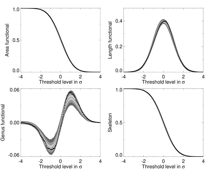
The three Minkowski functionals and the length of the skeleton, computed from maps smoothed with a Gaussian beam (Kp0 base mask), are shown in Figure 4. The WMAP data are plotted with black filled circles, while the median computed from the ensemble of 5000 Monte Carlo simulations is shown as a thin solid line. The 1, 2, and confidence bands around the median are shown as gray bands. However, in all cases except the genus, the confidence regions are so narrow that it is virtually impossible to distinguish between the different elements.
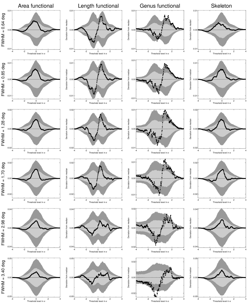
For this reason, we subtract in what follows the median from each bin before plotting the functions, and such results are shown for the full-sky measurements in Figure 5. In these plots there are several points worth noticing: First, we see that the genus confidence bands are asymmetric in the tails. This is because of the inability of our method to deal with masks; i.e., on a cut sky, the number of maxima plus the number of minima minus the number of saddle-points is likely to be non-zero, and this translates in our method into a non-zero genus at . On the other hand, there are no stationary points at very high thresholds (when the remaining area of the sky is very small); therefore, the genus will always be zero here. However, this asymmetry is only a very minor problem for thresholds between and , and the effect is in any case calibrated by simulations.
Second, the plots show that the properties of the full-sky field on scales up to are in fairly good agreement with the model. No single function shows excessive deviations, but the deviations are also not too small compared to the confidence bands, as could easily be the case if the power spectrum was flawed. However, the genus curve does seem to have a somewhat large amplitude, and more so at large scales. At FWHM the genus lies clearly outside the band.
In order to quantify the degree of deviation in each case, we use the diagonal statistic described in §5. The results from these measurements are shown in Table 3 (for the Kp0 base mask) and Table 4 (for the larger base mask). The numbers in these tables indicate the percentage of simulations with a lower value than that of the observed WMAP data. Once again we see that the full-sky numbers are in excellent agreement with the Gaussian theoretical model, except for the genus at large (–) scales, which has a that is high at the 96% level.
| FWHM | Area | Length | Genus | Skeleton |
|---|---|---|---|---|
| Full sky | ||||
| 49.4% | 67.8% | 86.2% | 23.4% | |
| 43.9% | 65.2% | 88.3% | 28.6% | |
| 35.2% | 56.8% | 89.4% | 35.4% | |
| 26.9% | 44.3% | 89.3% | 29.3% | |
| 23.5% | 34.8% | 86.0% | 28.4% | |
| 21.5% | 29.1% | 79.5% | 24.8% | |
| 19.9% | 19.1% | 77.5% | 20.8% | |
| 16.2% | 13.8% | 69.3% | 16.6% | |
| 12.5% | 10.8% | 95.9% | 11.3% | |
| 8.2% | 7.6% | 94.3% | 8.1% | |
| ** computed only for thresholds between and . | 4.3% | 3.1% | 80.5% | 7.8% |
| Northern hemisphere | ||||
| 12.5% | 34.5% | 95.9% | 14.4% | |
| 15.4% | 32.5% | 95.3% | 15.1% | |
| 14.1% | 24.6% | 97.2% | 18.9% | |
| 9.6% | 26.7% | 95.7% | 13.8% | |
| 9.4% | 30.6% | 98.4% | 18.4% | |
| 13.1% | 34.6% | 98.4% | 23.0% | |
| 17.7% | 35.3% | 99.5% | 20.3% | |
| 20.3% | 29.6% | 94.9% | 32.2% | |
| ** computed only for thresholds between and . | 28.3% | 29.4% | 77.3% | 40.1% |
| Southern hemisphere | ||||
| 33.5% | 54.9% | 27.7% | 33.6% | |
| 53.2% | 70.9% | 37.7% | 58.4% | |
| 59.2% | 64.0% | 43.0% | 67.0% | |
| 58.6% | 65.7% | 28.8% | 55.9% | |
| 58.6% | 71.4% | 19.4% | 54.6% | |
| 54.2% | 70.5% | 85.2% | 49.5% | |
| 51.4% | 66.6% | 57.6% | 43.9% | |
| 45.0% | 56.3% | 21.8% | 35.5% | |
| ** computed only for thresholds between and . | 39.6% | 40.4% | 9.6% | 32.2% |
Note. — Area functional, length functional, and genus results from diagonal tests, as computed from values of the threshold between and . The numbers indicate the percentage of simulated realizations with a value lower than that for the co-added WMAP map using the Kp0 mask.
| FWHM | Area | Length | Genus | Skeleton |
|---|---|---|---|---|
| Northern hemisphere | ||||
| 22.5% | 48.0% | 97.6% | 22.6% | |
| 11.3% | 49.8% | 99.2% | 20.2% | |
| 9.2% | 49.8% | 99.9% | 33.2% | |
| 10.6% | 46.0% | 94.5% | 29.5% | |
| 12.3% | 40.2% | 62.2% | 24.5% | |
| ** computed only for thresholds between and . | 12.1% | 27.5% | 42.0% | 16.5% |
| Southern hemisphere | ||||
| 31.5% | 18.7% | 16.6% | 35.9% | |
| 36.2% | 12.7% | 1.0% | 36.8% | |
| 31.5% | 7.2% | 34.1% | 36.3% | |
| 34.6% | 13.6% | 17.1% | 25.0% | |
| 33.5% | 16.2% | 96.8% | 19.2% | |
| ** computed only for thresholds between and . | 32.0% | 15.5% | 78.9% | 6.1% |
Note. — Same as Table 3, but where all areas with have been included in the mask.
This pattern is clearly stronger in the northern hemisphere. Here the genus generally is very large, with a pronounced peak at . At that scale only 0.5% of the simulations have a larger . The other functionals are all perfectly acceptable. In the southern hemisphere, even the genus is acceptable, and no signs of discrepancy between the observed sky and the simulations are found there. We see that these results are not particularly dependent on the choice of base mask, except that with the larger mask, the genus peaks at FWHM in the northern hemisphere, rather than at , and that it is curiously low at in the southern hemisphere (at the 1% level). However, it is difficult to attach much significance to the latter result, since it is highly unstable with respect to both Galactic cut and smoothing scale.
The statistic only measures the overall level of deviation between a given function and the theoretical mean. It is possible that other statistics could be more sensitive to particular features. To study the behavior of the genus in more detail, we therefore fit the parametric function given by Equation (24) to each realization (Park, 2004), allowing for non-zero shifts and arbitrary amplitudes. The results from these computations are shown in Tables 5 (Kp0 base mask) and 6 (larger base mask). Only the amplitudes and the asymmetry parameters are shown; the shift parameters are in all cases well inside the range, except for the smallest scales ( and FWHM) . The number in parentheses here shows the percentage of the simulated maps having the fitted parameter smaller than for the WMAP data.
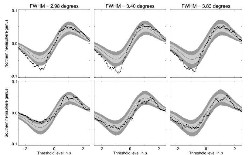
We see that the genus amplitude (and especially when fitted for in the range to , i.e., ) is very high in the northern hemisphere and relatively small in the southern hemisphere, compared with the simulations. In particular, the scale once again stands out as special ( scale with the base mask); in the northern hemisphere the negative threshold amplitude is so large that only 1 out of 5000 simulations has a larger amplitude. Using the larger base mask, no simulations have as large as the WMAP map at FWHM. In adition, the asymmetry parameter is clearly large at the level in the northern hemisphere.
| FWHM | ||||
|---|---|---|---|---|
| Full sky | ||||
| 0.087 (87.3%) | 0.086 (82.6%) | 0.091 (98.0%) | -0.024 (5.5%) | |
| 0.092 (87.4%) | 0.090 (79.3%) | 0.096 (98.9%) | -0.034 (2.3%) | |
| 0.091 (91.5%) | 0.089 (86.4%) | 0.094 (98.3%) | -0.027 (8.1%) | |
| 0.082 (91.9%) | 0.080 (85.4%) | 0.087 (98.4%) | -0.038 (10.3%) | |
| 0.078 (90.4%) | 0.076 (84.2%) | 0.084 (98.6%) | -0.049 (11.3%) | |
| 0.080 (95.3%) | 0.080 (93.8%) | 0.080 (94.4%) | 0.000 (53.9%) | |
| 0.082 (96.4%) | 0.083 (96.0%) | 0.080 (92.2%) | 0.018 (67.5%) | |
| 0.081 (93.6%) | 0.083 (92.9%) | 0.083 (93.8%) | -0.001 (55.2%) | |
| 0.095 (99.5%) | 0.101 (99.6%) | 0.081 (86.8%) | 0.111 (93.5%) | |
| 0.096 (99.1%) | 0.104 (99.5%) | 0.081 (82.0%) | 0.128 (93.2%) | |
| 0.094 (96.9%) | 0.097 (96.1%) | 0.091 (93.9%) | 0.031 (67.7%) | |
| Northern hemisphere | ||||
| 0.100 (97.5%) | 0.099 (96.9%) | 0.104 (99.7%) | -0.021 (18.3%) | |
| 0.090 (93.9%) | 0.089 (91.0%) | 0.094 (98.4%) | -0.027 (20.4%) | |
| 0.091 (97.9%) | 0.091 (96.6%) | 0.092 (97.7%) | -0.004 (47.3%) | |
| 0.095 (98.7%) | 0.097 (98.8%) | 0.087 (89.4%) | 0.056 (85.4%) | |
| 0.104 (99.9%) | 0.110 (99.9%) | 0.085 (81.0%) | 0.132 (97.6%) | |
| 0.110 (99.9%) | 0.120 (99.9%) | 0.085 (76.8%) | 0.170 (98.3%) | |
| 0.122 (99.9%) | 0.134 (99.9%) | 0.092 (85.7%) | 0.188 (97.5%) | |
| 0.116 (99.5%) | 0.129 (99.7%) | 0.086 (65.8%) | 0.204 (97.0%) | |
| 0.113 (97.7%) | 0.123 (98.0%) | 0.094 (77.3%) | 0.136 (87.2%) | |
| Southern hemisphere | ||||
| 0.084 (23.3%) | 0.081 (15.5%) | 0.088 (46.3%) | -0.039 (5.6%) | |
| 0.077 (38.6%) | 0.074 (26.6%) | 0.081 (58.9%) | -0.044 (10.7%) | |
| 0.070 (26.1%) | 0.066 (15.9%) | 0.078 (60.7%) | -0.083 (4.4%) | |
| 0.069 (28.7%) | 0.065 (19.4%) | 0.076 (54.0%) | -0.076 (12.4%) | |
| 0.068 (27.0%) | 0.062 (16.8%) | 0.077 (57.9%) | -0.108 (9.2%) | |
| 0.058 (7.6%) | 0.047 (2.4%) | 0.083 (69.9%) | -0.271 (0.4%) | |
| **The two large cold spots discussed by Park (2004) are masked out. | 0.064 (16.0%) | 0.054 (6.5%) | 0.094 (89.2%) | -0.269 (0.9%) |
| 0.078 (54.2%) | 0.082 (63.3%) | 0.067 (20.3%) | 0.100 (86.0%) | |
| 0.082 (58.6%) | 0.083 (60.7%) | 0.077 (43.2%) | 0.036 (65.4%) | |
| 0.086 (63.2%) | 0.083 (55.4%) | 0.089 (67.8%) | -0.038 (43.3%) | |
Note. — The fitted amplitude of the genus for the full range in , for negative , and for positive , and the genus asymmetry parameter, using the co-added WMAP map with Kp0 mask. The numbers in parentheses show the percentage of the 5000 simulations with a value smaller than for the WMAP map.
| FWHM | ||||
|---|---|---|---|---|
| Northern hemisphere | ||||
| 0.106 (99.4%) | 0.110 (99.4%) | 0.094 (88.8%) | 0.079 (88.6%) | |
| 0.115 (99.8%) | 0.124 (99.9%) | 0.091 (76.7%) | 0.155 (97.0%) | |
| 0.131 (99.9%) | 0.144 (100%) | 0.095 (79.8%) | 0.206 (97.8%) | |
| 0.125 (99.5%) | 0.137 (99.6%) | 0.101 (83.0%) | 0.151 (90.8%) | |
| 0.117 (95.4%) | 0.129 (96.2%) | 0.099 (73.2%) | 0.132 (83.5%) | |
| 0.120 (93.4%) | 0.131 (92.8%) | 0.106 (77.2%) | 0.107 (75.6%) | |
| Southern hemisphere | ||||
| 0.078 (43.7%) | 0.077 (40.9%) | 0.084 (64.0%) | -0.044 (27.7%) | |
| 0.079 (46.2%) | 0.079 (44.5%) | 0.081 (48.5%) | -0.014 (45.7%) | |
| 0.068 (15.3%) | 0.064 (14.1%) | 0.077 (32.8%) | -0.088 (21.2%) | |
| 0.077 (33.6%) | 0.082 (45.6%) | 0.065 (10.3%) | 0.117 (85.6%) | |
| 0.108 (89.1%) | 0.127 (96.6%) | 0.064 (8.4%) | 0.334 (99.6%) | |
| 0.104 (79.1%) | 0.123 (90.8%) | 0.069 (13.0%) | 0.279 (97.5%) | |
Note. — Same as Table 5, but with all areas with added to the mask.
In the southern hemisphere, the genus amplitudes are relatively, but not extremely, low. However, here the asymmetry parameter is rather small, at the 99% level, for smoothing and use of the Kp0 base mask. This result is in fact quite peculiar, and it is difficult to decide how much significance one should attach to it; it is very sensitive to smoothing scale, and it is not seen in the larger base mask measurement. One could suspect that this result is caused by some features near the Galactic plane. However, we have not been able to locate any region that by exclusion brings the results to an acceptable level. One example from this search is shown in Table 5, marked by an asterisk. In this case we have removed two disks of radius centered on and , corresponding to the two large cold spots discussed by Park (2004). Obviously, the peculiar 99% result is not connected to these regions.
The genus for both the northern and the southern hemispheres at , , and FWHMs is shown in Figure 6. Here we clearly see the origin of the extreme numbers found above: the northern hemisphere genus at around FWHM lies well outside the lower confidence region and even outside the region for an extended range of thresholds. In addition, the genus has a very small amplitude at negative thresholds on the southern hemisphere, but an average amplitude at positive thresholds, resulting in a rather extreme asymmetry parameter.
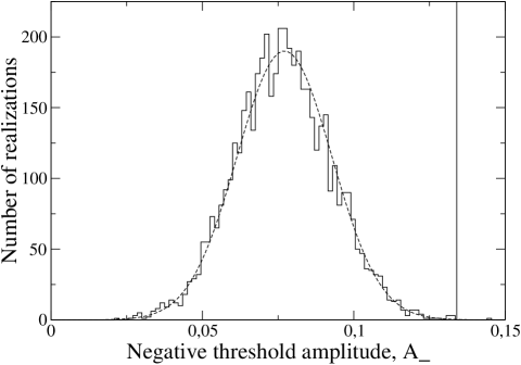
The distribution of negative threshold amplitudes for the northern hemisphere at FWHM is shown for the 5000 simulations in Figure 7, together with the observed WMAP value of 0.134 (vertical line). The distribution is close to Gaussian with a mean of 0.0771 and a standard deviation of 0.0157. Thus, the observed WMAP -value is formally larger than the simulations at . However, this number is likely to be slightly overestimated: since the amplitude is a strictly positive number, we should expect the true distribution to be somewhat skewed toward large values. On the other hand, this effect cannot be very significant in our case, given the good fit between the histogram and the Gaussian approximation. The case seems solid for rejecting the null hypothesis at considerably more than confidence.
6.3. Comparison with alternative maps
So far we have only studied the co-added WMAP map, which is dominated by the -band. The influence of residual foregrounds could therefore be an important concern when interpreting these results. In order to study this issue closer, we now reestimate the northern hemisphere statistics (using the Kp0 mask), this time for a set of seven different maps: (1) the co-added WMAP map, (2) the Tegmark et al. cleaned map (Tegmark, de Oliveira-Costa, & Hamilton 2003), (3) the WMAP Internal Linear Combination (ILC) map (Bennett et al., 2003b), (4)–(6) the averaged -, - and -bands, and (7) a synchrotron-corrected map [defined by ; see Vielva et al. 2004)].
Each of these maps has its own effective beam profile, and in order for a direct comparison to be meaningful, we have to pre-smooth each map so that they have a common resolution. This was achieved by first deconvolving the old beam and subsequently convolving with a Gaussian beam. The only exception is the ILC map, which is already smoothed to the appropriate resolution.
The simulations that we carry out in this paper are very CPU-intensive, and it would therefore be very time consuming to perform a complete analysis of each of the above-mentioned maps. However, after pre-smoothing each map to a common resolution, only the effect of noise can potentially modify the results, and on the large scales that we consider, this effect is very small. We may therefore instead use the existing simulations when interpreting the new results.
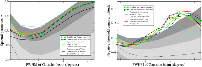
The two panels of Figure 8 show the results from this analysis for the spectral parameter and the negative threshold genus amplitude . Each panel contains two sets of fundamentally different elements. First, the gray 1, 2, and confidence regions and the light green curve with green filled circles (the co-added WMAP map) show the results of §6.2 and are thus not pre-smoothed to resolution. The seven remaining curves correspond to the maps listed above and are pre-smoothed.
The effect of the pre-smoothing operation may be reconstructed by comparing the two green curves (with circles and with diamonds), which show the results for the co-added WMAP map, un-smoothed and smoothed, respectively. For the spectral parameter (left panel), we see that the pre-smoothing process effectively suppresses on small scales, but increases it very slightly on large scales. However, this effect is both small and stable on large scales, and is thus not difficult to account for. The effect on the genus amplitude (right panel) is slightly less predictable but follows the same pattern; the pre-smoothed function lies generally a little higher than the un-smoothed function on large scales.
The main conclusion to be drawn from these plots, however, is that the quantities discussed above show a remarkable stability with respect to both frequency and foreground correction method. If we neglect the synchrotron-corrected map and the WMAP ILC map, we see that the scatter in is much less than , as seen by the width of the confidence regions. The same is true for the genus amplitude on the scale of most interest, namely, FWHM. We note that the WMAP team warns (see the LAMBDA Web site) that the ILC map should not be used for CMB studies, and indeed it is the most deviant with respect to the other maps in the analysis.
The final issue to consider is the effect of point sources. We therefore now apply a median filter to the co-added map, compute the same set of quantities for this filtered map, and compare the results to those of the unfiltered map. Our median filter is implemented by replacing each pixel value that is excluded by the WMAP point-source mask, i.e., the mask consisting of about 700 disks of radius, by the median evaluated over a disk around that pixel. Such filters are commonly used in, e.g., radio astronomy, to eliminate outliers.
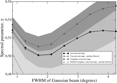
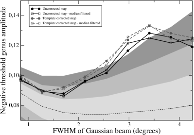
The results from this experiment are shown in Figure 9. Once again, we plot and estimated in the northern hemisphere (Kp0 mask), since these quantities represent the two strongest detections presented in this paper. The results are shown for two different maps, the raw co-added map and the WMAP template-corrected map. In both cases the effect of the median filter may be seen by comparing the solid and dashed lines (circles and squares), which correspond to the raw map and the median filtered map, respectively.
It is apparent that median filtering changes by a negligible amount on large scales while on small scales is very slightly decreased. The effect on the genus amplitude is less predictable, as the two curves lie both above and below each other. However, it is interesting to note that the filtered maps are associated with a slightly larger amplitude than the raw maps at FWHM and a slightly smaller amplitude at FWHM. Of course, it is difficult to estimate the significance of this. In any case, it is clear that the impact of point sources is too small to explain the reported large-scale results in this paper.
6.4. Correlations between the measurements
In the previous sections we presented measurements of several important statistics. In this section we go one step further and seek to understand the correlations between some of these statistics. This goal is important both in order to understand the nature of the quantities themselves and for assessing the combined significance of the quoted results. In the following we focus on the full-sky measurements smoothed with a FWHM Gaussian beam.
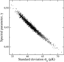
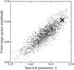
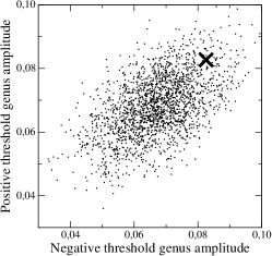
Figure 10 shows the following scalar quantities plotted pair-wise against each other: the temperature standard deviation versus the spectral parameter , the spectral parameter versus the full range genus amplitude , and the negative threshold genus amplitude versus the positive threshold amplitude . The values from each simulated realization are marked by a small filled circle, and the WMAP results are marked by a cross.
In Figure 10a we see that the correlation between and is very strong and negative. Of course, given that , this is no surprise. Nevertheless, it is well worth noticing that the spectral parameter may in many respects be identified with the standard deviation of the map.
Figure 10b demonstrates the clear correlation between the spectral parameter and the full range genus amplitude . Although the scatter is non-negligible, a high -value is probably accompanied by a large genus amplitude. Thus, given the large -value of WMAP, the large observed genus amplitude seen in both Table 5 and Figure 5 is not unexpected.
Finally, in Figure 10c we see that there is only a very weak correlation between the negative threshold genus amplitude and the positive threshold amplitude .
The conclusions to be drawn from these plots are therefore the following:
-
•
The spectral parameter is almost inversely proportional to the standard deviation of the map.
- •
-
•
The negative and positive threshold genus amplitudes are only very mildly correlated.
Given these relations, we may now make a few connections between the results presented in §6.2. First, we noted that the WMAP spectral parameter was large in both the full-sky measurements and particularly the northern hemisphere. However, it was not significantly different from the simulations in the southern hemisphere. These results are thus in perfect agreement with the genus measurements shown in Figures 5 and 6, and the parameters given in Table 5 — both and the genus amplitudes are large in the northern hemisphere, but fully acceptable in the southern hemisphere. The measurements of and the genus amplitudes may obviously not be regarded as independent.
One further interesting connection may be made through the relation between and the standard deviation , which may be taken as a very crude measure of the overall power in the map, determined primarily by the large-scale modes. Since is very large in the northern hemisphere, the standard deviation is very small; in other words, there is little power in this region. This result therefore supports the conclusions of Eriksen et al. (2004), that there is a clear lack of large-scale power in the northern hemisphere. Conversely, the genus results are generally stronger than the results, and given the relatively high results, a complete explanation must probably be formulated as a combination of power spectrum and other non-Gaussianity effects.
7. Conclusions
In this paper we have presented the three two-dimensional Minkowski functionals and the length of the skeleton of the co-added WMAP map, as well as a number of other statistics, and compared these with simulations based on Gaussian perturbations with a best-fit power spectrum and WMAP-specific noise and beam properties. On scales between and , all the statistics except for the genus Minkowski functional accept the model. On scales smaller than there are too many stationary points, a result that is interpreted as an effect of point sources.
By studying each Galactic hemisphere separately, it was found that on scales around , the northern hemisphere deviates significantly from the simulations. Most importantly, the genus functional has a very large amplitude on these scales; only 1 Monte Carlo realization out of 5000 simulations has a larger amplitude for negative thresholds. Interestingly, the southern hemisphere genus has a fairly small amplitude around the same scales. Furthermore, the spectral parameter is higher in the WMAP data than in the simulations on scales in the northern hemisphere. These asymmetries may be compared with those recently announced by Eriksen et al. (2004) and Park (2004). Park also reports an asymmetry in the genus amplitudes between the northern and southern hemispheres. However, these results are found on significantly smaller scales than those considered here, and it is therefore difficult to establish a direct link between our findings and those of Park (2004).
Many of the results presented in this paper depend on both the power spectrum and the higher-order statistical properties of the field. For example, the genus amplitude depends to a large extent on the power spectrum, and the strong results found on the northern hemisphere may therefore be influenced by both power spectrum and non-Gaussianity issues. However, the asymmetry parameter, , is a much cleaner test of non-Gaussianity, and we found that this was extreme at the 99% level in the southern hemisphere in a few cases. This result may therefore be taken as support for the results presented by Vielva et al. (2004), who find non-Gaussian signatures in the southern hemisphere using spherical wavelets. However, the WMAP parameter is also large at the level in the north around FWHM, and this is not supported by the results of Vielva et al. (2004). It is therefore quite difficult to determine if our results support the previously reported non-Gaussian effects, or whether these findings are independent.
It is in any case clear that the currently accepted Gaussian model has problems accounting for the statistical properties of the WMAP data on large and intermediate scales. In this paper we have focused particularly on the co-added WMAP data, but have also shown that the results are very stable with respect to frequencies and different foreground correction methods. Thus, uncertainties in foreground contributions or residuals are unlikely to resolve these issues. While it certainly is too early to conclude that these detections are of primordial origin, the possibility should certainly be taken into account. The 2-year WMAP data, and eventually the Planck data, will be essential in determining the nature of these detections.
References
- Bennett et al. (2003a) Bennett, C. L. et al. 2003a, ApJS, 148, 1
- Bennett et al. (2003b) Bennett, C. L. et al. 2003b, ApJS, 148, 97
- Bernardeau & Uzan (2003) Bernardeau, F., & Uzan, J.-F. 2003, Phys. Rev. D, 67, 121301(R)
- Bouchet et al. (2002) Bouchet, F. R., Peter, P., Riazuelo, A., & Sakellariadou, M. 2002, Phys. Rev. D, 65, 021301(R)
- Coles (1988) Coles, P. 1988, MNRAS, 234, 509
- Coles & Barrow (1987) Coles, P., & Barrow, J. D. 1987, MNRAS, 228, 407
- Coles et al. (2004) Coles, P., Dineen, P., Earl, J., & Wright, D. 2004, MNRAS, 350, 989
- Colley & Gott (2003) Colley, W. N., & Gott, J. R. 2003, MNRAS, 344, 686
- Copi et al. (2004) Copi, C. J., Huterer, D., & Starkman, G. D. 2004, Phys. Rev. D, 70, 043515
- Eriksen et al. (2004) Eriksen, H. K., Hansen, F. K., Banday, A. J., Górski, K. M., & Lilje, P. B. 2004, ApJ, 605, 14
- Górski et al. (1999) Górski, K. M., Hivon, E., & Wandelt, B. D., 1999, in Evolution of Large-Scale Structure: From Recombination to Garching, ed. A. J. Banday, R. K. Sheth, & L. N. da Costa (Garching: ESO), 37
- Gott, Melott, & Dickinson (1986) Gott, J. R., Melott, A. L., & Dickinson, M. 1986, ApJ, 306, 341
- Gott et al. (1990) Gott, J. R., Park, C., Juszkiewicz, R., Bies, W. E., Bennett, D. P., Bouchet, F. R., & Stebbins, A. 1990, ApJ, 352, 1
- Hadwiger (1957) Hadwiger, H. 1957, Vorlesungen über Inhalt, Oberfläche und Isoperimetrie (Berlin: Springer)
- Hansen et al. (2004) Hansen, F. K., Cabella, P., Marinucci, D., & Vittorio, N. 2004, ApJ, 607, L67
- Hinshaw et al. (2003) Hinshaw, G. et al. 2003, ApJS, 148, 135
- Komatsu et al. (2003) Komatsu, E. et al. 2003, ApJS, 148, 119
- Lyth & Wands (2002) Lyth, D. H., & Wands, D. 2002, Physics Letters B, 524, 5
- Minkowski (1903) Minkowski, H. 1903, Mathematische Annalen, 57, 447
- Naselsky et al. (2003) Naselsky, P. D., Verkhodanov, O. V., Chiang, L.-Y., & Novikov, I. D. 2003, ApJ, submitted (astro-ph/0310235)
- Novikov et al. (2003) Novikov, D., Colombi, S., & Doré, O., 2003, MNRAS, submitted (astro-ph/0307003)
- Novikov, Feldman, & Shandarin (1999) Novikov, D., Feldman, H. A., & Shandarin, S. F. 1999, Int. J. Mod. Phys. D, 8, 291
- Novikov et al. (2000) Novikov, D., Schmalzing, J., & Mukhanov, V. F. 2000, A&A, 364, 17
- Park (2004) Park, C.-G. 2004, MNRAS, 349, 313
- Schmalzing & Górski (1998) Schmalzing, J., & Górski, K. M. 1998, MNRAS, 355
- Shandarin et al. (2002) Shandarin, S. F., Feldman, H. A., Xu, Y., & Tegmark, M. 2002, ApJS, 141, 1
- Spergel et al. (2003) Spergel, D. N. et al. 2003, ApJS, 148, 175
- Tegmark et al. (2003) Tegmark, M., de Oliveira-Costa, A., & Hamilton, A. 2003, Phys. Rev. D, 68, 123523
- Vielva et al. (2004) Vielva, P., Martínez-González, E., Barreiro, R. B., Sanz, J. L., & Cayón, L. 2004, ApJ, 609, 22
- Wang & Kamionkowski (2000) Wang, L., & Kamionkowski, M. 2000, Phys. Rev. D, 61, 063504
- Winitzki & Kosowsky (1998) Winitzki, S, & Kosowsky, A. 1998, New Astronomy, 3, 75