A Preliminary Seismic Analysis of 51 Peg: Large and Small Spacings from Standard Models

Abstract

We present a preliminary theoretical seismic study of the astronomically famous star 51 Peg. This is done by first performing a detailed analysis within the Hertzsprung-Russell diagram (HRD). Using the Yale stellar evolution code (YREC), a grid of stellar evolutionary tracks has been constructed for the masses $1.00M_{\odot},1.05M_{\odot}$ and $1.10M_{\odot}$, in the metallicity range $Z=0.024-0.044$, and for values of the Galactic helium enrichment ratio ($\Delta Y/\Delta Z$) in the range 0-2.5. Along these evolutionary tracks, we select 75 stellar model candidates that fall within the 51 Peg observational error box in the HRD (all turn out to have masses of $1.05M_{\odot}$ and $1.10M_{\odot}$). The corresponding allowable age range for these models, which depends sensitively on the parameters of the model, is relatively large and is $\sim$2.5 - 5.5 Gyr. For each of the 75 models, a non-radial pulsation analysis is carried out, and the large and small frequency spacings are calculated. The results show that just measuring the large and small frequency spacings will greatly reduce the present uncertainties in the derived physical parameters and in the age of 51 Peg. Finally we discuss briefly refinements in the physics of the models and in the method of analysis which will have to be included in future models to make the best of the precise frequency determinations expected from space observations.

1 Introduction

With current stellar structure and evolution theories, the placement of a star on the Hertzsprung-Russell diagram (HRD) does not allow a complete stellar parameterization. This stems from the fact that, except for the Sun, the number of free parameters is higher than the number of observables. We therefore look at seismology for additional observables to remove this degeneracy and to perform a more thorough analysis.

Traditional observations of nearby stars lead to a range in uncertainties for stellar radii and luminosity. In the best cases an accuracy of $1\%-10\%$ is attainable (Demarque et al. 1986). And with current modeling of stellar evolution, the stellar ages are not known better than $\pm 10\%-25\%$. However, with the help of seismology, it is expected that the uncertainty levels will be significantly reduced (Guenther 1998).

At the simplest level of detection, even when it is not feasible to determine individual frequencies, it is often possible to identify two quantities in the stellar p-mode oscillation spectrum, the large and small frequency spacings (Tassoul 1980). These quantities are defined in §3.1 below. As shown by Christensen-Dalsgaard (1984), these two quantities can be used to constrain the radius and age of the star, provided its chemical composition is known (Ulrich 1986). Thus the large and small frequency spacings can provide important tests of the theory of stellar structure and evolution for stars whose chemical composition and distance are known.

We now take the case of the relatively well-studied nearby star 51 Peg and attempt to constrain its basic parameters by combining stellar evolution modeling and stellar pulsation calculations. 51 Peg (HD 217014, HR 8729, HIP 113357) is classified as a G2.5IVa (Hoffleit 1982). It is best known for the discovery that it harbors an extra-solar, Jupiter-like planet (Mayor & Queloz 1995; Marcy & Butler 1998). The excitement associated with the planetary system of 51 Peg has placed it high on the target list for upcoming space missions. One mission of special interest is the recently launched Canadian MOST (Microvariability and Oscillation of STars) microsatellite which has begun observing a number of stars (Matthews et al. 2000), including 51 Peg. We present this analysis in anticipation of the MOST observations.

This paper begins with the construction of stellar evolutionary tracks constrained by the conventional astronomical parameters for 51 Peg. Stellar models are then selected from these evolutionary tracks on the basis of whether or not they fall within the observational error box mapped for 51 Peg onto the HRD. These candidates are then pulsed and the calculated non-radial oscillation frequencies are used to derive both large and small p-mode frequency spacings. We show how, when combined with upcoming seismic data, the calculated large and small spacings will reduce the uncertainties in 51 Peg’s physical parameters and age estimate. Thus, the spacings will help us refine future stellar interior models for this star.

The organization of the paper goes as follows: In §2.1 we discuss the specifics of our models and the physics implemented for their calculations. Then in §2.2 we outline how we go on to use observational data to help constrain our models through our HRD analysis. §3 describes the calculation of both large and small p-mode spacings and how they can assist in constraining the parameters of 51 Peg. Lastly, in §4, we summarize our analysis, which is necessarily exploratory in the absence of seismic observations. Some shortcomings of our models which will have to be addressed when precise frequency measurements become available are discussed. Finally, we point out the need to devise more sophisticated approaches to analyze the high quality data expected from the space missions.

2 Stellar Models

2.1 Model Physics

All evolutionary tracks were computed using the Yale stellar evolution code (YREC) (Guenther et al. 1992). The initial zero age main sequence (ZAMS) model used for 51 Peg was created from pre-main sequence evolution calculations. Post-main sequence models of various compositions were then constructed by first rescaling the composition of the ZAMS models.

In constructing the models we made use of the current OPAL equation of state tables (Rogers et al.1996). OPAL tables (Iglesias & Rogers 1996) were also used to calculate interior opacities, while the surface and atmosphere opacities were taken from the work of Alexander and Ferguson (1994). Due to the lack of better information, we assume a solar mixture of heavy elements. We accounted for the diffusion of both the helium and heavy element abundances by weight (Y and Z, respectively), using the diffusion coefficients of Thoul et al. (1994), in the way described by Guenther & Demarque (1997) in their models of the Sun.

As expected, all the stellar models in this study exhibit a convective envelope. In such stellar models, the calculated pulsational frequencies are known to be sensitive to the treatment of the atmosphere and outer convective layers (Guenther et al. 1992; Robinson et al. 2003). In the atmosphere, we used the Eddington T-$\tau$ relation for a grey atmosphere, and the mixing length theory to describe convectively unstable layers (Böhm-Vitense 1958). The calculated radius also depends on the choice of the mixing length parameter $\alpha$ (mixing length to scale-height ratio). We set $\alpha$ = 1.7 for all models, close to the value required to reproduce the solar radius under the same physical assumptions and stellar evolution code. A fuller description of the treatment of the outer layers and of the constitutive physics incorporated into YREC can be found in Guenther et al. (1992).

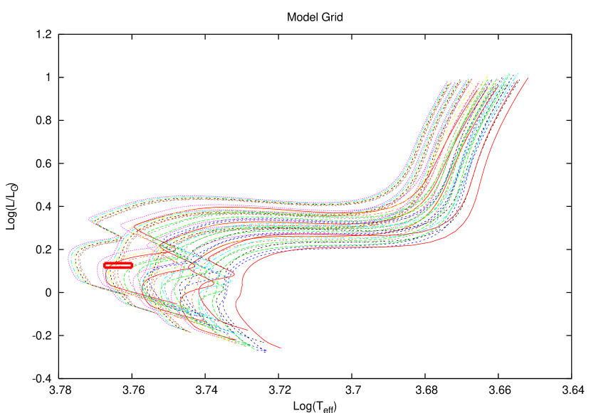
Inspection of the evolutionary tracks in Figure 1 shows evidence in some of the tracks for a hydrogen exhaustion phase indicative of the presence of a convective core near the main sequence. For simplicity, and because of the exploratory nature of this study, we have assumed in this study that no overshoot takes place at the edge of convective cores, i.e. we have set $\alpha_{OV}$ = 0.0, where $\alpha_{OV}$ is the core overshoot parameter. The main consequence of core overshoot is to shorten the evolutionary lifetime. Thus the presence of core overshoot would extend the core burning phase of evolution and increase the estimated age of 51 Peg (see e.g. Audard et al. 1995; Yi et al. 2000; Woo & Demarque 2001). This important topic will be the subject of a separate study.

2.2 Constraining Models with Observations

Table 1 lists the principal constraints from observation. They are the position of 51 Peg in the HRD, with the associated error box, and two quantities derived from spectroscopy, i.e. the metallicity [Fe/H] and surface gravity $g$ (Santos et al. 2003). The spectroscopic estimate of log $g$ is a relatively weak constraint which is easily satisfied since log $g$ changes little all along the main sequence.

In mapping the observables onto the HRD, we have calculated the luminosity of 51 Peg using the published visual magnitude in the Hipparcos catalog (Perryman et al. 1997). Error estimates were derived based on the associated Hipparcos parallax error. Assuming a solar bolometric magnitude of 4.75 mag, we then calculated the bolometric correction by linear interpolation in the color-correction tables of Green et al. (1987) in $T_{\rm eff}$, [Fe/H], and log g, to obtain our final estimate of $L_{\rm bol}$. No transformation of $T_{\rm eff}$ was necessary since it maps directly from observation onto the theoretical HRD. Thus we constructed an error box based on

$$L_{\rm bol}=1.343_{-0.037}^{+0.025}L_{\sun}$$ (1)

and,

$$T_{\rm eff}=5805\pm 50{\rm K}$$ (2)

which is shown in Figure 1. Where a star lies in the theoretical HRD ($L_{\rm bol}$ vs. $T_{\rm eff}$) is a complicated function of Y and Z, stellar mass, and age. In addition to the observational constraints from Table 1, the mass and helium content of 51 Peg are only approximately known. We used theoretical evolutionary tracks, as outlined in the next section, to better constrain these two parameters and to derive an age for 51 Peg. Only those models which fell inside the error box in the HRD were considered as possible candidates for 51 Peg.

2.3 Evolutionary Tracks and Candidates for Pulsation

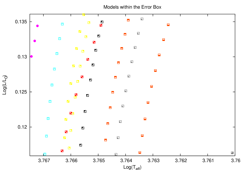
Table 2 lists the parameters adopted for the grid of evolutionary tracks. The heavy element content by mass, Z, was derived from [Fe/H]. The helium abundance Y, which cannot be observed directly, was taken to be solar with several plausible values of the nucleosynthetic helium enrichment parameter $\Delta Y/\Delta Z$ at higher Z. The position in the HRD and the measured log$~{}g$ suggested a mass in the vicinity of one solar mass or slightly higher. Thus our grid of stellar evolutionary tracks was constructed in the three parameter space of mass, Z, and $\Delta Y/\Delta Z$ given in Table 2. The complete calculated grid contained 45 evolutionary tracks of models for analysis. Having constructed the grid we further selected those models which we considered as candidates for pulsation on the basis of whether or not they landed within the observational error box in the theoretical HRD. This error box is shown in Figure 1. A total of 75 models fall within this region and are listed in Table 3.

We see in Table 3 that none of the 1.0 $M_{\sun}$ evolutionary tracks pass through the error box in the HRD. For the 1.05 $M_{\sun}$ tracks, only models for Z = 0.024 satisfy the HRD position constraint. In this case, the acceptable range in $\Delta Y/\Delta Z$ is 0.5-2.5. On the other hand, for the 1.10 $M_{\sun}$ models, the range of possible metallicities includes Z = 0.034-0.044, with correspondingly higher helium abundances.

We also note that on the basis of this analysis alone, the age of 51 Peg is still quite uncertain, and in the range $\sim$2.5 - 5.5 Gyr. For comparison, we recall previous age estimates of 8.5 Gyr, Noble et al. (2002), and 7.0 Gyr, quoted by Edvardsson et al. (1993) and Ng & Bertelli (1998). All these ages are based on sets of isochrones by VandenBerg (1985) and Bertelli et al. (1994), and for various reasons, appear to be overestimates. More recently, Gonzalez (1998) estimates $6\pm 2$ Gyr for the age and $1.05\pm 0.03M_{\odot}$ for the mass of 51 Peg on the basis of the Schaller et al. (1992) and Schaerer et al. (1992) isochrones.

In summary, for the purpose of this paper, and in view of the large uncertainties discussed above, we shall treat the 75 models listed in Table 3 as equally likely model candidates for 51 Peg. We shall see below that seismic observations of 51 Peg would greatly constrain parameters such as mass, age and metallicity.

3 Pulsation Analysis

We now go through the exercise of evaluating the p-mode frequencies of the 75 selected models using Guenther’s stellar pulsation code (Guenther 1994). It is important to remember that the theoretical frequencies calculated here should not be expected to match the observed frequencies of 51 Peg very closely. To start with, our theoretical models do not match either the radius or mass of 51 Peg precisely. But even in the hypothetical case in which the model radius and mass reproduce the stellar radius and mass with high precision (as in a calibrated standard solar models), the calculated frequencies could still differ appreciably from the observed frequencies due to the uncertainty in calculating the sound speed in the outer layers of the models where non-adiabatic effects become important. For instance, in the case of standard solar models constructed under the same physical assumptions as the 51 Peg models we present, this discrepancy can reach 10-20 $\mu Hz$ at the higher frequencies (see Guenther & Demarque 1997; Winnick et al. 2001). This discrepancy is reduced by a factor of four in standard solar models that include a more realistic description of convection in the atmosphere (Li et al. 2002). Because the discrepancies are themselves a function of frequency, these could also result in a smaller but significant effect on the calculated large spacings discussed in §3.2 and §4.

On the other hand, the small spacings, being primarily sensitive to the central concentration of the model, are less affected by the details of the surface boundary conditions. The small spacings are sensitive primarily to age and to the size of the convective core when one is present.

3.1 Generating $p$-Mode Frequencies and Spacings

Guenther’s (1994) pulsation code allows for the non-adiabatic corrections in the pulsation needed to account for radiation in the Eddington approximation. The accuracy of these corrections is a function of frequency such that at high frequencies it is harder to account for non-adiabatic effects due to convection-oscillation interactions and thus errors are larger. We define the large spacings $\Delta\nu$ and small spacings $\delta\nu$ in the usual way, such that,

$$\Delta\nu_{\it{n,l}}\equiv\nu(n,l)-\nu(n-1,l)$$ (3)

and,

$$\delta\nu_{\it{n,l}}\equiv\nu(n,l)-\nu(n-1,l+2),$$ (4)

where n is the radial order, l is the azimuthal order, and $\nu$ is the frequency. The importance of these spacings and association with upcoming observations is discussed in §3.2 and §3.3.

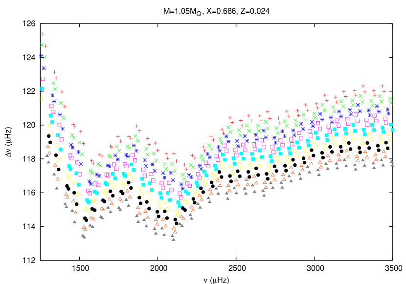
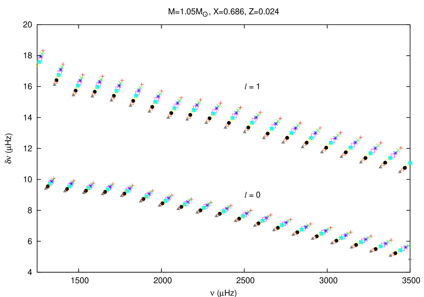
Large and small spacings were obtained over the ranges of $n=1-30$ and $l=0-3$. These values of n and l correspond to a frequency range of $\sim 1000\mu$Hz to $\sim 4000\mu$Hz. We, however, only plot the frequency range out to $\sim 3500\mu$Hz due to the expected acoustic cutoff just beyond this limit.

In Table 3 we give the parameters of each model along with characteristic large and small spacings. The mean large spacings are averages over $\ell$ = 0,1,2,3 and $n$ = 10,11,12,…,30. The mean small spacings are averages over $n$ = 10,11,12,…,30 at a fixed $\ell$. For illustration, we have plotted in Figures 2 and 3, average large and small spacings respectively vs. frequency for a given subset of nine individual stellar models along the evolutionary track having M $=1.05M_{\sun}$, X $=0.686$, and Z $=0.024$, which fell within our error box.

3.2 Large Spacings

It is well known from asymptotic theory that the large spacings are mainly sensitive to the stellar radius (Tassoul 1980; Christensen-Dalsgaard 1984). More precisely, the asymptotic behavior of $\Delta\nu$ is expected to scale with $(M/R^{3})^{1/2}$ where M is the mass of the star and R is its radius. It is therefore not surprising that perturbations in Y and Z will have less effect on the large spacings than uncertainties in the luminosity and $T_{\rm eff}$ $(L\propto R^{2}T_{\rm eff}^{4}$).

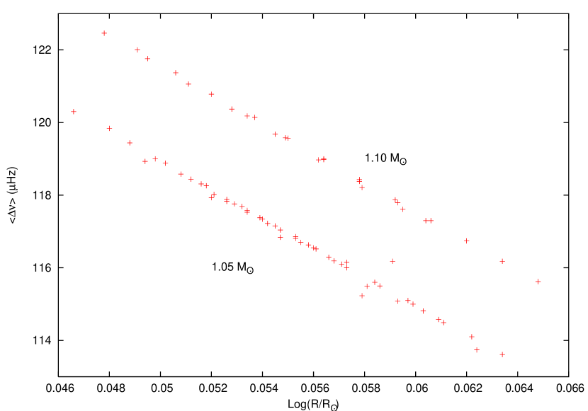
As pointed out by Guenther (1998), one of the most easily identifiable characteristics in the p-mode spectrum are the large spacings. They are seen as a peak in the Fourier transform of the power spectrum and because they are mostly uncontaminated by composition effects, these large separations provide a much more precise way to measure stellar radii compared with conventional techniques. In Figure 4 we plot the average large spacings vs. model radius.

It is clear from the plot that radius increases as $\Delta\nu$ decreases with very little scatter for the 1.05 $M_{\sun}$ models. We find that a degeneracy in predicted radius occurs for models of different mass. Specifically, in our analysis, we see that $\Delta\nu$ calculated from 1.10$M_{\sun}$ models lie on a nearly parallel line to that generated by the 1.05$M_{\sun}$ models having a vertical shift of around 2.7$\mu$Hz in $\Delta\nu$ and a much larger scatter. Such a shift implies that an observed $\Delta\nu$ can lead to the calculation of a radius differing by nearly $\sim.007R_{\sun}$ depending on whether the stellar mass is 1.05 $M_{\sun}$ or 1.10 $M_{\sun}$. This degeneracy may be lifted by using solar models with the assumption of a homologous scaling.

It is sometimes convenient to assume homology to compare theoretical models by introducing a “reduced” radius (see e.g. Fernandes and Monteiro 2003) such that,

$$\Delta\nu_{r}=\Delta\nu_{n,l}\left(\frac{R}{R_{\sun}}\right)^{3/2},$$ (5)

We have listed the values of $\Delta\nu_{r}$ for each model in Table 3.

It is easily seen that the values of the “reduced” spacings are relatively consistent for each mass such that $\Delta\nu_{r}\sim 141\mu$Hz for 1.05 $M_{\sun}$ models and $\Delta\nu_{r}\sim 144\mu$Hz for 1.10 $M_{\sun}$. Were our stellar models purely homologous, then the reduced spacing would only be a function of mass. This would then lead us to calculate the correct mass when $\Delta\nu_{r}=\Delta\nu_{\sun}$. We could therefore obtain a correct radius for 51 Peg from the $\Delta\nu$ versus radius plot. Note however that this is only approximately true. Scatter exists within the calculated $\Delta\nu_{r}$ due to significant departure from homology between the solar interior structure and the models for 51 Peg. These fluctuations in $\Delta\nu_{r}$ are due to variations in chemical composition and age, as well as other input physics of each model such as the depth of the convection zone. Direct measurements of stellar diameters from interferometric observations may be able to help provide an independent check with these asteroseismic predictions (Boden et al. 1998; Kervella et al. 2003a,b).

3.3 Small Spacings

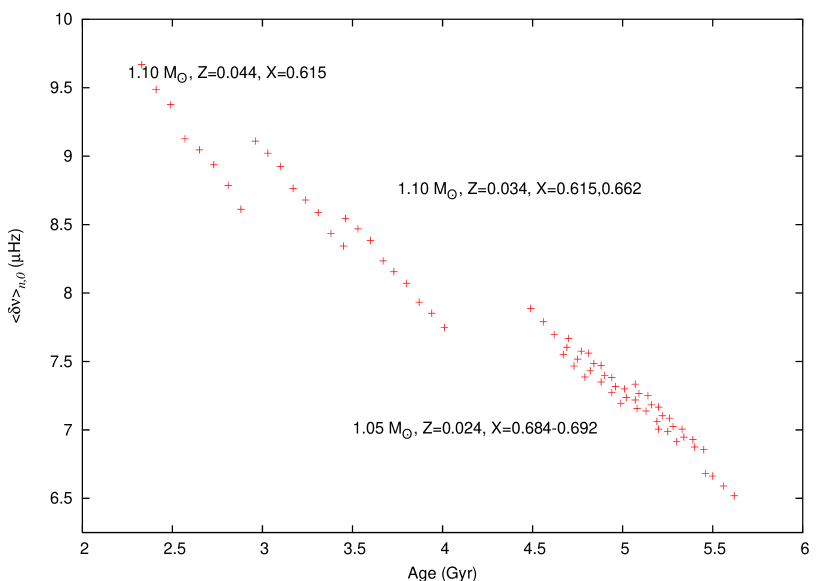
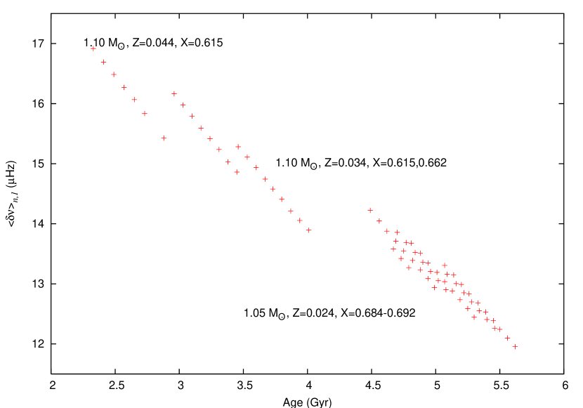
As mentioned earlier, it was initially believed that the calculation of small spacings could put a constraint on the age of the star (Christensen-Dalsgaard 1984). However, it was subsequently realized that only if the composition of the star is known completely can one use the small spacings to correctly identify a stellar age unequivocally (Ulrich 1986). This point is illustrated in Figure 5, where we plot the average small spacings vs. the calculated age for all potential 51 Peg model candidates. It is obvious that the models of different chemical compositions each define a distinct locus of points which seems to follow offset linear relationships such that age increases with decreasing $\delta\nu$. Each locus of model points at each composition seem to have very nearly the same slope, but shifted both vertically and horizontally. Thus, the various chemical compositions create a degeneracy in age determination.

The small spacings, like the large spacings, will be visible as peaks in the Fourier transform of the power spectrum. However, as Figure 5 clearly shows, the small spacings seem rather sensitive to composition and therefore to the structure of the core. The extreme sensitivity of the stellar core density stratification to several parameters has been discussed in the case of $\alpha$ Cen A (Kim 1999; Guenther & Demarque 2000; Morel et al. 2000). Though sensitive to composition, the small spacings can still be used to further constrain the models and obtain a radius once precise observations are available. The measurement of the small spacing will enable us to constrain the mass in Figure 5 to a much narrower range than is presently possible on the basis of HRD position alone. Note that there is an extremely small overlap in $\delta\nu$ for stars with 1.05 $M_{\sun}$ and 1.10 $M_{\sun}$. Given an observed small spacing, one could determine more precisely which range of models to use to calculate the radius in Figure 4. Thus, by obtaining both small and large spacings it is possible in principle to reduce considerably the $\Delta\nu$-radius degeneracy with mass, and to reduce the age uncertainty to less than 1.0 Gyr.

4 Summary and conclusions

Using the constraints from the best available observations of the star’s position in the HRD, as well as the available spectroscopic constraints on its metallicity and surface gravity, we have made an analysis of the pulsation properties of a set of evolutionary models for the star 51 Peg. All of these models were selected from the evolutionary tracks for their location within the HRD error box of 51 Peg. These evolutionary tracks covered a range of metallicities. (Note that spectroscopy also provided an estimate of the surface gravity, a weaker constraint, but a useful consistency check in this case). In order to construct the tracks, two additional parameters had to be chosen , the helium abundance, and the mass. The adopted composition and mass parameters for the 45 evolutionary tracks are given in Table 2.

Table 3 lists the acceptable models for 51 Peg. The range in stellar parameter space through the initial survey within the HRD is relatively large. In this case, the conventional astronomical tests leave a mass uncertainty of about $5\%$ and a large range in age $(2.5-5.5Gyr$).

Thus it is clear that p-mode observations, even at the most basic level, will aid in the analysis of stellar evolution and structure. We have outlined the usefulness of both the calculation of the large and small spacings as well as discuss how both can be used in conjunction with one another to lift existing degeneracies in detailed stellar parameterization. In particular, since the large p-mode spacings are primarily sensitive to radius while insensitive to composition, they will, along with precise parallax measurements, provide improvements in the calculation of stellar radii and $T_{\rm eff}$. And, as a result, it should be possible to reduce the uncertainty in age to less than 1 Gyr.

We emphasize that the expected high quality and quantity of the space observations, including the precise measurements of individual oscillation mode frequencies, will necessitate more sophisticated stellar models than presented in this paper. As pointed out by Guenther & Demarque (2000) in the case of $\alpha$ Cen A, quality seismic data can reveal the presence of a convective core, either at this time or during the past evolution of the star, and the size of the mixed region. This important point has recently been made more graphically by Guenther & Brown (2004). Observations from space will be needed to settle this issue. The recent ground-based observations (Bouchy & Carrier 2002; Carrier & Bourban 2003) of individual frequencies in $\alpha$ Cen A and B have improved our knowledge of the system, but the uncertainties are still such that interior models constructed with those data have yet to reach a consensus (Thévenin et al. 2002; Thoul et al. 2003).

Two significant effects with seismic signatures should be included in future models of 51 Peg, i.e. convective core overshoot, and turbulence in the outer layers of the convection zones. The extent of core overshoot may be detectable from the small frequency spacings and from the signature of mode bumping. The detailed comparison of individual mode frequencies will also require taking into account the effects of turbulence in the outer convectively unstable layers in the stellar models which shift the observed frequencies. The parameterization of turbulence tested on the Sun by Li et al. (2002) can be applied to models for Sun-like stars as well. This parameterization can be extended to other stars by using the three-dimensional radiative hydrodynamical simulations of Robinson et al. (2003), which are based on the same microscopic physics, and can readily be parameterized in the YREC stellar evolution code. We intend to explore both the effects of convective core overshoot and of including turbulence in modeling the outer layers in subsequent papers. We now await the first results from MOST on 51 Peg to compare our theory to observations.

At the same time, high quality observations from space will also require more powerful techniques of analysis than we have used to interpret the observations and take advantage of the wealth of information contained in a spectrum of well determined frequencies (Brown et al. 1984). Powerful new approaches are being developed to extract precise masses and metallicities (Guenther & Brown 2004) and envelope helium abundances (Basu et al. 2003) for individual stars from precisely measured pulsation frequencies.

Figure 1: To the left, we plot our initial grid of evolutionary tracks (45 in total) in the theoretical HRD, spanning the parameter values listed in Table 2. The observational error box is drawn. To the right, we plot a blow-up of the error box showing the 75 acceptable individual stellar models along each track. Parameters of the models are listed in Table 3.

Figure 2: Large frequency spacings vs. frequency for 9 individual stellar models (models 4-12 in Table 3) along the evolutionary track with parameters: $M=1.05M_{\sun}$, $X=0.686$, and $Z=0.024$.

Figure 3: Small frequency spacings vs. frequency for the same 9 stellar models as in Fig.2. Spacings for $\ell=0$ and $\ell=1$ are marked.

Figure 4: Average calculated large frequency spacings vs. stellar radius (in solar units) for each of the 75 stellar models.

Figure 5: Average calculated small frequency spacings vs. age for each of the 75 stellar models. The left-hand panel shows the spacings for $\ell=0$, the right-hand panel for $\ell=1$.

Table 1: Observational Data of 51 Peg

Observable	Value	Source
$T_{\rm eff}$	5805 $\pm$ 50K	Santos et al. 2003
log g	4.51 $\pm$ 0.15 dex	Santos et al. 2003
$\pi$ (″)	0.06510 $\pm$ 0.00076	Hipparcos Catalog
$[$Fe/H$]$	0.21 $\pm$ 0.06 dex	Santos et al. 2003

Table 2: Input Parameters for Model Tracks

Variable	minimum value	maximum value	$\delta$
$M/M_{\sun}$	1.00	1.10	0.05
Z	0.024	0.044	0.01
$\Delta$Y/$\Delta$Z	0.0	2.5	0.5

Note. — $\delta$ defines the increment between minimum and maximum parameter values used to create the model array.

Table 3: Model Parameters

Star	M	X	$\Delta$Y/$\Delta$Z	Z	Log Teff	Log L	Log R	Age	$<$$\Delta\nu$$>$	$<$$\delta\nu$$>$	$<$$\delta\nu$$>$	$<$$\Delta\nu_{r}$$>$
	($M_{\sun}$)					($L_{\sun}$)	($R_{\sun}$)	(Gyr)		(n,0)	(n,1)
1	1.05	0.684	2.50	0.0240	3.7675	0.128	0.0526	4.67	117.83	7.5502	13.579	141.33
2	1.05	0.684	2.50	0.0240	3.7674	0.130	0.0539	4.73	117.38	7.4667	13.422	141.42
3	1.05	0.684	2.50	0.0240	3.7673	0.132	0.0553	4.79	116.86	7.3860	13.269	141.44
4	1.05	0.686	2.00	0.0240	3.7670	0.113	0.0466	4.49	120.30	7.8876	14.224	141.29
5	1.05	0.686	2.00	0.0240	3.7670	0.116	0.0480	4.56	119.84	7.7898	14.047	141.43
6	1.05	0.686	2.00	0.0240	3.7669	0.119	0.0494	4.62	118.93	7.6952	13.878	141.05
7	1.05	0.686	2.00	0.0240	3.7668	0.121	0.0508	4.69	118.58	7.6040	13.711	141.30
8	1.05	0.686	2.00	0.0240	3.7668	0.124	0.0521	4.75	118.02	7.5165	13.549	141.29
9	1.05	0.686	2.00	0.0240	3.7667	0.126	0.0534	4.82	117.53	7.4320	13.391	141.34
10	1.05	0.686	2.00	0.0240	3.7666	0.128	0.0547	4.88	116.84	7.3498	13.235	141.16
11	1.05	0.686	2.00	0.0240	3.7665	0.130	0.0560	4.94	116.55	7.2716	13.087	141.43
12	1.05	0.686	2.00	0.0240	3.7664	0.133	0.0573	4.99	116.15	7.1941	12.938	141.57
13	1.05	0.688	1.50	0.0240	3.7661	0.114	0.0488	4.70	119.44	7.6681	13.857	141.36
14	1.05	0.688	1.50	0.0240	3.7661	0.117	0.0502	4.77	118.88	7.5753	13.688	141.38
15	1.05	0.688	1.50	0.0240	3.7660	0.120	0.0516	4.84	118.31	7.4847	13.522	141.37
16	1.05	0.688	1.50	0.0240	3.7659	0.122	0.0529	4.90	117.76	7.3989	13.361	141.36
17	1.05	0.688	1.50	0.0240	3.7658	0.124	0.0542	4.96	117.22	7.3162	13.206	141.38
18	1.05	0.688	1.50	0.0240	3.7658	0.126	0.0555	5.02	116.70	7.2359	13.053	141.38
19	1.05	0.688	1.50	0.0240	3.7657	0.129	0.0568	5.08	116.19	7.1570	12.902	141.38
20	1.05	0.688	1.50	0.0240	3.7656	0.131	0.0581	5.14	115.49	$\cdots$	$\cdots$	141.14
21	1.05	0.688	1.50	0.0240	3.7654	0.133	0.0593	5.20	115.08	7.0054	$\cdots$	141.25
22	1.05	0.689	1.00	0.0240	3.7657	0.115	0.0498	4.81	119.00	7.5607	13.678	141.36
23	1.05	0.689	1.00	0.0240	3.7656	0.117	0.0512	4.88	118.44	7.4708	13.512	141.37
24	1.05	0.689	1.00	0.0240	3.7656	0.120	0.0526	4.94	117.88	7.3822	13.347	141.37
25	1.05	0.689	1.00	0.0240	3.7655	0.122	0.0540	5.01	117.34	7.2997	13.192	141.38
26	1.05	0.689	1.00	0.0240	3.7654	0.124	0.0553	5.07	116.81	7.2187	13.037	141.39
27	1.05	0.689	1.00	0.0240	3.7653	0.127	0.0566	5.13	116.29	7.1378	12.883	141.39
28	1.05	0.689	1.00	0.0240	3.7652	0.129	0.0579	5.19	115.23	7.0621	12.736	140.72
29	1.05	0.689	1.00	0.0240	3.7651	0.131	0.0591	5.25	116.18	6.9868	12.589	142.48
30	1.05	0.689	1.00	0.0240	3.7650	0.133	0.0603	5.30	114.81	6.9136	12.445	141.41
31	1.05	0.691	0.50	0.0240	3.7648	0.116	0.0520	5.03	117.93	$\cdots$	$\cdots$	141.16
32	1.05	0.691	0.50	0.0240	3.7647	0.118	0.0534	5.09	117.58	7.2654	13.160	141.40
33	1.05	0.691	0.50	0.0240	3.7647	0.120	0.0547	5.16	117.04	7.1834	13.004	141.40
34	1.05	0.691	0.50	0.0240	3.7646	0.123	0.0561	5.22	116.52	7.1034	12.852	141.41
35	1.05	0.691	0.50	0.0240	3.7645	0.125	0.0573	5.28	116.00	7.0238	12.699	141.41
36	1.05	0.691	0.50	0.0240	3.7644	0.127	0.0586	5.34	115.50	6.9478	12.551	141.41
37	1.05	0.691	0.50	0.0240	3.7643	0.129	0.0599	5.40	115.00	6.8747	12.407	141.42
38	1.05	0.691	0.50	0.0240	3.7641	0.131	0.0611	5.46	114.49	6.6822	12.261	141.40
39	1.05	0.691	0.50	0.0240	3.7640	0.133	0.0624	5.51	113.74	$\cdots$	$\cdots$	141.07
40	1.05	0.692	0.50	0.0240	3.7644	0.114	0.0518	5.07	118.26	7.3337	13.307	141.40
41	1.05	0.692	0.50	0.0240	3.7643	0.116	0.0532	5.14	117.69	7.2495	13.148	141.41
42	1.05	0.692	0.50	0.0240	3.7643	0.118	0.0545	5.20	117.15	7.1661	12.989	141.41
43	1.05	0.692	0.50	0.0240	3.7642	0.121	0.0558	5.26	116.63	7.0860	12.835	141.42
44	1.05	0.692	0.50	0.0240	3.7641	0.123	0.0571	5.33	116.10	7.0058	12.682	141.42
45	1.05	0.692	0.50	0.0240	3.7640	0.125	0.0584	5.39	115.60	6.9293	12.533	141.42
46	1.05	0.692	0.50	0.0240	3.7639	0.127	0.0597	5.45	115.10	6.8553	12.387	141.44
47	1.05	0.692	0.50	0.0240	3.7638	0.129	0.0609	5.50	114.58	6.6625	12.242	141.42
48	1.05	0.692	0.50	0.0240	3.7637	0.131	0.0622	5.56	114.10	6.5905	12.098	141.42
49	1.05	0.692	0.50	0.0240	3.7635	0.133	0.0634	5.62	113.61	6.5189	11.954	141.43
50	1.10	0.615	2.50	0.0440	3.7665	0.114	0.0478	2.33	122.46	9.6681	16.917	144.45
51	1.10	0.615	2.50	0.0440	3.7663	0.117	0.0495	2.41	121.76	9.4855	16.692	144.44
52	1.10	0.615	2.50	0.0440	3.7662	0.119	0.0511	2.49	121.06	9.3758	16.485	144.44
53	1.10	0.615	2.50	0.0440	3.7660	0.122	0.0528	2.57	120.37	9.1264	16.270	144.45
54	1.10	0.615	2.50	0.0440	3.7658	0.125	0.0545	2.65	119.68	9.0453	16.067	144.45
55	1.10	0.615	2.50	0.0440	3.7656	0.127	0.0562	2.73	118.97	8.9367	15.834	144.45
56	1.10	0.615	2.50	0.0440	3.7654	0.130	0.0579	2.81	118.21	8.7847	$\cdots$	144.36
57	1.10	0.615	2.50	0.0440	3.7652	0.132	0.0595	2.88	117.61	8.6115	15.426	144.46
58	1.10	0.656	2.00	0.0340	3.7663	0.116	0.0491	2.96	122.00	9.1095	16.163	144.53
59	1.10	0.656	2.00	0.0340	3.7662	0.118	0.0506	3.03	121.37	9.0214	15.977	144.54
60	1.10	0.656	2.00	0.0340	3.7662	0.121	0.0520	3.10	120.78	8.9242	15.793	144.54
61	1.10	0.656	2.00	0.0340	3.7661	0.124	0.0534	3.17	120.18	8.7645	15.593	144.54
62	1.10	0.656	2.00	0.0340	3.7660	0.126	0.0549	3.24	119.58	8.6796	15.416	144.54
63	1.10	0.656	2.00	0.0340	3.7659	0.129	0.0564	3.31	118.98	8.5877	15.237	144.55
64	1.10	0.656	2.00	0.0340	3.7658	0.131	0.0578	3.38	118.38	8.4349	15.030	144.54
65	1.10	0.656	2.00	0.0340	3.7657	0.134	0.0593	3.45	117.79	8.3435	14.861	144.55
66	1.10	0.662	1.50	0.0340	3.7635	0.114	0.0537	3.46	120.14	8.5445	15.281	144.60
67	1.10	0.662	1.50	0.0340	3.7635	0.116	0.0550	3.53	119.57	8.4686	15.109	144.60
68	1.10	0.662	1.50	0.0340	3.7634	0.119	0.0564	3.60	119.00	8.3837	14.936	144.61
69	1.10	0.662	1.50	0.0340	3.7633	0.121	0.0578	3.67	118.43	8.2343	14.744	144.60
70	1.10	0.662	1.50	0.0340	3.7632	0.123	0.0592	3.73	117.87	8.1555	14.578	144.61
71	1.10	0.662	1.50	0.0340	3.7630	0.126	0.0606	3.80	117.30	8.0715	14.408	144.61
72	1.10	0.662	1.50	0.0340	3.7629	0.128	0.0620	3.87	116.74	7.9327	14.212	144.61
73	1.10	0.662	1.50	0.0340	3.7628	0.130	0.0634	3.94	116.18	7.8519	14.055	144.61
74	1.10	0.662	1.50	0.0340	3.7626	0.132	0.0648	4.01	115.62	7.7468	13.894	144.62
75	1.10	0.669	1.00	0.0340	3.7602	0.114	0.0604	4.15	117.30	$\cdots$	$\cdots$	144.51

Note. — The above mean large spacings were calculated averaging over $l=0,1,2,3$ and $n=10,11,12,...,30$. The mean small spacings were averages over $n=10,11,12,...,30$ at a fixed l (as indicated)

References

- Alexander & Ferguson (1994) Alexander, D. R. & Ferguson, J. W. 1994, ApJ, 437, 879
- Audard et al. (1995) Audard, N., Provost, J. & Christensen-Dalsgaard, J. 1995, A&A, 297, 427
- Basu et al. (2004) Basu, S., Mazumdar, A., Antia, H.M., & Demarque, P. 2004, MNRAS, accepted
- Böhm-Vitense (1958) Böhm-Vitense, E. 1958, ZAp, 46, 108
- Boden et al. (1998) Boden, A. F., van Belle, G. T., Colavita, M. M., et al. 1998, ApJ, 504, L39
- Bertelli et al. (1994) Bertelli, G., Bressan, A., Chiosi, C., Fagotto, F., & Nasi, E. 1994, A&AS, 106, 275
- Bouchy & Carrier (2002) Bouchy, F. & Carrier, F. 2002, A&A, 390, 205
- Brown et al. (1984) Brown, T.M., Christensen-Dalsgaard, J., Weibel-Mihalas, B., & Gilliland, R.L. 1994, ApJ, 427, 1013
- Carrier & Bourban (2003) Carrier, F. & Bourban, G. 2003, A&A, 406, L23
- Christensen-Dalsgaard (1984) Christensen-Dalsgaard, J. in Space Research Prospects in Stellar Activity and Variability, eds. A. Mangeney and F. Praderie (Meudon: Obs. de Paris-Meudon), p. 11
- Demarque et al. (1986) Demarque, P., Guenther, D. B., & van Altena, W. F. 1986, ApJ, 300,773
- Fernandes & Monteiro (2003) Fernandes, J. & Monteiro, M. J. P. G. 2003 A&A, 399, 243
- Edvardsson et al. (1993) Edvardsson, B., Andersen, J., Gustafsson, B., Lambert, D.L., Nissen, P.E., & Tomkin, J. 1993, A&A, 275, 101
- Gonzalez (1998) Gonzalez, G. 1998, A&A, 334, 221
- Green et al. (1987) Green, E. M., Demarque, P., & King, C. R. 1987, The Revised Yale Isochrones and Luminosity Functions (New Haven: Yale Univ. Obs.)
- Guenther (1994) Guenther, D. B. 1994, ApJ, 422, 400
- Guenther (1998) Guenther, D. B. 1998, in Proc. SOHO 6/GONG 98 Workshop, Structure and Dynamics of the Interior of the Sun and Sun-like Stars, ed S. Korzennik & A. Wilson (ESA SP-418), 375
- Guenther & Brown (2004) Guenther, D.B. & Brown, K.I.T. 2004, ApJ, in press
- Guenther et al. (1992) Guenther, D. B., Demarque, P., Kim, Y.-C., & Pinsonneault, M. H. 1992, ApJ, 387, 372
- Guenther & Demarque (1997) Guenther, D.B. & Demarque, P. 1997, ApJ, 484, 937
- Guenther & Demarque (2000) Guenther, D. B. & Demarque P. 2000, ApJ, 531, 503
- Hoffleit (1982) Hoffleit, D. 1982, The Bright Star Catalogue, 4th edn. (Yale University Observatory, New Haven)
- Iglesias & Rogers (1996) Iglesias, C.A. & Rogers, F.J. 1996, ApJ, 464, 943
- Kervella et al. (2003) Kervella, P., Thévenin, F., Morel, P., Bordé, P., Di Folco, E. 2003a, A&A, 408, 681
- Kervella et al. (2003) Kervella, P., Thévenin, F., Ségransan, D., Berthomieu, G., Lopez, B., Morel, P., Provost, J. 2003b, A&A, 404, 1087
- Kim (1999) Kim, Y. -C. 1999, JKAS, 32, 119
- Li et al. (2002) Li, L.H., Robinson, F.J., Demarque, P., Sofia, S., & Guenther, D.B. 2002, ApJ, 567, 1192
- Marcy & Butler (1998) Marcy, G.W. & Butler, R.P. 1998, ARA&A, 36, 57
- Matthews et al. (2000) Matthews, J.M., Kuschnig, P., Walker, G.A.H. et al. 2000, in The Impact of Large Scale Surveys on Pulsating Star Research, ASP Conf. Ser. Vol. 203, eds. L. Szabados & D. Kurtz, p. 74
- Mayor & Queloz (1995) Mayor, M. & Queloz, D. 1995 Nature, 378, 355
- Morel et al. (2000) Morel, P., Provost, J.,Lebreton, Y., Thévenin, F., & Berthomieu, G. 2000, A&A, 363, 675
- Ng & Bertelli (1998) Ng Y. K. & Bertelli, G. 1998, A&A, 329, 943
- Noble et al. (2002) Noble, M., Musielak, Z. E., and Cuntz, M. 2002, ApJ, 572, 1024
- Perryman et al. (1997) Perryman, M.A.C., Lindegren, L., Kovalevsky, J. et al. 1997, A&A, 323, 49
- Robinson, F.J. et al. (2003) Robinson, F.J., Demarque, P., Li, L.H., Sofia, S., Kim, Y.-C., Chan, K.L. & Guenther, D.B. 2003, MNRAS, 340, 923
- Rogers, Swenson, & Iglesias (1996) Rogers, F. J., Swenson, F. J., & Iglesias, C. A. 1996, ApJ, 456, 902
- Santos et al. (2003) Santos, N. C., Israelian, G., Mayor, M., Rebolo, R., & Udry, S. 2003, A&A, 398, 363
- Tassoul (1980) Tassoul, M. 1980, ApJS, 43, 469
- Thévenin et al. (2002) Thévenin, F., Provost, J., Morel, P., Berthomieu, G., Bouchy, F. & Carrier, F. 2002, A&A, 392, L9
- Thoul et al. (1994) Thoul, A.A., Bahcall, J.N. & Loeb, A. 1994, ApJ, 421, 828
- Thoul, A. et al. (2003) Thoul, A., Scufflaire, R., Noels, A., Vatovez, B., Briquet, M., Dupret, M.-A. & Montalban, J. 2003, A&A, 402, 293
- Ulrich (1986) Ulrich, R. K. 1986, ApJ, 306, L37
- VandenBerg (1985) VandenBerg, D.A. 1985, ApJS, 58, 711
- Winnick,R.A et al. (2002) Winnick, R.A., Demarque,P., Basu, S., Guenther, D.B. 2002, ApJ, 576, 1075
- Woo & Demarque, P. (2001) Woo, J.-H. & Demarque, P. 2001, AJ, 122, 1602
- Yi et al. (2001) Yi, S., Demarque, P., Kim, Y.-C., Lee, Y.-W., Ree, C.H., Lejeune, Th. & Barnes, S. 2001, ApJS, 136, 417