Statistical properties of the combined emission of a population of discrete sources: astrophysical implications

Abstract

We study the statistical properties of the combined emission of a population of discrete sources (e.g. X-ray emission of a galaxy due to its X-ray binaries population). Namely, we consider the dependence of their total luminosity $L_{\rm tot}=\sum L_{k}$ and of fractional $rms_{\,\rm tot}$ of their variability on the number of sources $n$ or, equivalently, on the normalization of the luminosity function. We show that due to small number statistics a regime exists, in which $L_{\rm tot}$ grows non-linearly with $n$, in an apparent contradiction with the seemingly obvious prediction $\left<L_{\rm tot}\right>=\int L\,\frac{dN}{dL}\,dL\propto n$. In this non-linear regime, the $rms_{\,\rm tot}$ decreases with $n$ significantly more slowly than expected from the $rms\propto 1/\sqrt{n}$ averaging law. For example, for a power law luminosity function with a slope of $\alpha=3/2$, in the non-linear regime, $L_{\rm tot}\propto n^{2}$ and the $rms_{\,\rm tot}$ does not depend at all on the number of sources $n$. Only in the limit of $n\rightarrow\infty$ do these quantities behave as intuitively expected, $L_{\rm tot}\propto n$ and $rms_{\,\rm tot}\propto 1/\sqrt{n}$. We give exact solutions and derive convenient analytical approximations for $L_{\rm tot}$ and $rms_{\,\rm tot}$.

Using the total X-ray luminosity of a galaxy due to its X-ray binary population as an example, we show that the $L_{X}-$SFR and $L_{X}-M_{*}$ relations predicted from the respective “universal” luminosity functions of high and low mass X-ray binaries are in a good agreement with observations. Although caused by small number statistics the non-linear regime in these examples extends as far as SFR$\la 4-5$ M_⊙/yr and $\log(M_{*}/M_{\odot})\la 10.0-10.5$, respectively.

1 Introduction and qualitative consideration

In many astrophysical situations a problem arises to predict or interpret results of measurements of the total (combined) luminosity of a population of discrete sources. Among many examples are the total luminosity of X-ray binaries in a galaxy, or total flux of background sources detected above the sensitivity limit inside the field of view of a telescope.

In the following discussion we will use high mass X-ray binaries (HMXB) in star forming galaxies as an example. As was shown by Grimm, Gilfanov & Sunyaev (2003), the luminosity distribution of HMXB sources in a galaxy is described to first approximation by a ”universal” luminosity function whose shape is the same in all galaxies and whose normalization is proportional to the star formation rate (SFR) of the parent galaxy:

$$\frac{dN}{dL}\propto{\rm SFR}\times f(L)$$ (1)

In a broad luminosity range, $\log(L_{X})\sim 35.5-40.5$, the shape of the HMXB “universal” luminosity function is close to a power law, $f(L)=L^{-\alpha}$, with the slope of $\alpha\approx 1.6$. Importantly, the luminosity of the compact sources in star forming galaxies appears to be restricted by a maximum value of $L_{\rm cut}\sim{\rm few}\times 10^{40}$ erg/s. This cut-off luminosity can be defined, for example, by the Eddington luminosity limit for the most massive objects associated with the star forming regions. Obviously, on the faint side, the luminosity distribution eq.(1) must become flatter or have a cut-off as well, in order to keep the total number of sources finite. This low luminosity cut-off may be caused for example by the propeller effect (, 1975) as discussed by Shtykovskii & Gilfanov (2004).

The expectation value for the total number of sources in a galaxy equals

$$\left<N_{\rm tot}\right>=\int_{0}^{+\infty}\frac{dN}{dL}dL\propto{\rm SFR}$$ (2)

and, naturally, is directly proportional to its star formation rate. The number of sources actually observed in a given galaxy obeys Poisson distribution $p_{\mu}(N)$ with $\mu$ defined by eq.(2). Apart from effects of counting statistics, the number of HMXB sources found in an arbitrarily chosen galaxy will be close to the above expectation value.

The problem, considered in this paper, is the behavior of the total luminosity of high mass X-ray binaries in a galaxy

$$L_{\rm tot}=\sum_{k=1}^{k=N}L_{k}$$ (3)

as a function of its star formation rate.

An apparently obvious expression for the $L_{\rm tot}$ can be obtained integrating the luminosity distribution (1):

$$\left<L_{\rm tot}\right>=\int_{0}^{+\infty}L\,\frac{dN}{dL}\,dL\propto{\rm SFR}$$ (4)

Hence, one might expect that the total X-ray luminosity of HMXB sources is also directly proportional to the star formation rate of the host galaxy, as is the total number of sources. This problem, however, involves some subtleties related to the statistical properties of the power law distribution of the sources over luminosity, which appear not to have been recognized previously, at least in astrophysical context (a somewhat related problem has been considered by Kalogera et al. 2001 in connection with estimating the coalescence rate for the NS–NS binaries in the Galaxy). Although eq.(4) correctly predicts the average X-ray luminosity computed for a large number of galaxies with similar values of star formation rate, it fails to describe the relation between the most probable value of X-ray luminosity of an arbitrarily chosen galaxy and its SFR. The main surprise of the study presented here is that, in the low SFR regime, the relation between SFR of the host galaxy and the total luminosity of its HMXBs is non-linear – with increase of the star formation rate the luminosity appears to grow faster than linear. The relation becomes linear only for sufficiently high star formation rates, when the total number of objects with a luminosity close to the maximum possible value, defined by $L_{\rm cut}$, becomes sufficiently large.

This can be illustrated by the following simple consideration. For an arbitrarily chosen galaxy, the brightest source is most likely going to have a luminosity $\tilde{L}_{\rm max}$ defined by the condition

$$N(L>\tilde{L}_{\rm max})=\int_{\tilde{L}_{\rm max}}^{+\infty}\frac{dN}{dL}\,dL\sim 1$$ (5)

For a power law luminosity distribution with slope $\alpha$ and with a cut-off at $L_{\rm cut}$, eq.(1), the above expression yields:

$$\begin{array}[]{lll}\tilde{L}_{\rm max}&\propto SFR^{\ \frac{1}{\alpha-1}}&\mbox{low SFR}\\ \tilde{L}_{\rm max}&=L_{\rm cut}&\mbox{high SFR}\end{array}$$ (8)

As might be intuitively expected, at low SFR, the most probable luminosity of the brightest source increases with SFR, until it reaches the maximum value of $L_{\rm cut}$. The threshold value of the star formation rate, separating low and high SFR regimes, is defined by the condition $N(L\sim L_{\rm cut})\sim 1$, i.e. that there are $\sim$few sources expected, with luminosity close to the cut-off value $L_{\rm cut}$.

The most probable value of the total luminosity, $\tilde{L}_{\rm tot}$ can be then computed integrating the luminosity function from $L_{min}$ to $\tilde{L}_{\rm max}$:

$$\tilde{L}_{\rm tot}\approx\int^{\tilde{L}_{\rm max}}_{L_{min}}\frac{dN}{dL}L~{}dL$$ (9)

which, for $1<\alpha<2$ and $L_{\rm min}<<\tilde{L}_{\rm max}$, leads to

$$\tilde{L}_{\rm tot}\propto\left\{\begin{array}[]{ll}SFR^{\frac{1}{\alpha-1}}&\mbox{low SFR}\\ SFR&\mbox{high SFR}\end{array}\right.$$ (12)

i.e. is non-linear in the low SFR regime and becomes linear only at high star formation rates.

This can be qualitatively understood as follows. For a slope of the luminosity distribution $1<\alpha<2$, the total luminosity of a galaxy is defined by the brightest sources. The non-linear behavior in the low-SFR limit is caused by the fact that an increase of the SFR leads to non-linear increase of the luminosity of the brightest sources. Therefore their total luminosity grows faster than the star formation rate. This non-linear growth continues until the maximum possible value of the luminosity of the compact sources is achieved. Further increase of the star formation rate leads to a linear increase of the number of the brightest sources in the galaxy, but not of their individual luminosities. Consequently, the $L_{X}-$SFR relation becomes linear.

In the more formal language of statistics such a behavior is related to the properties of the probability distribution of the collective luminosity $p\,(L_{\rm tot})$. In particular, it can be understood in terms of the difference between the expectation mean and the mode of the probability distribution. The expectation mean is defined as

$$\left<L_{\rm tot}\right>=\int_{0}^{\infty}p\,(L_{\rm tot})\,L_{\rm tot}\,dL_{\rm tot}$$ (13)

and is given by eq.(4). The mode of the statistical distribution, $\tilde{L}_{\rm tot}$, is defined as the value of the random variable ($L_{\rm tot}$ in our case) at which the probability distribution $p\,(L_{\rm tot})$ reaches its maximum value. Whereas the expectation mean $\left<L_{\rm tot}\right>$ describes the result of averaging of the X-ray luminosities of many galaxies having similar values of SFR, it is the mode of the $p\,(L_{\rm tot})$ distribution that predicts the most probable value of the total luminosity of a randomly chosen galaxy. The non-linear behavior in the low SFR regime is caused by the skewness of the probability distribution $p\,(L_{\rm tot})$ resulting in a difference between expectation mean and mode. In the high SFR limit, the $p\,(L_{\rm tot})$ distribution asymptotically approaches the Gaussian distribution, in accord with the Central Limit Theorem. The boundary value of SFR, separating the non-linear and linear regimes of the $L_{X}-$SFR relation is defined by the parameters of the luminosity function.

Interestingly, the fact of the existence of a linear regime in the $L_{X}$–SFR relation is a direct consequence of the cut-off in the luminosity function. Only in the presence of a maximum possible luminosity for the sources, $L_{\rm cut}$, (for instance Eddington limit for a neutron star) a linear regime can exist, when the total luminosity of a galaxy is defined by a sufficiently large number of bright sources near $L_{\rm cut}$, and any subsequent increase of the star formation rate results in linear growth of the total luminosity.

In the above discussion, we used high mass X-ray binary populations in star forming galaxies as an example. Obviously, the effect considered in this paper is of a broader general interest and is at work in many situations related to computing/measuring integrated luminosity of a finite number of discrete sources. One example related to the application of stellar synthesis models to observations of stellar clusters has been independently discovered by Cervino & Luridana (2004).

The paper is structured as follows. In section 2 we consider the statistical properties of the total luminosity, in particular in section 2.1 derive the formulae for the probability distribution $p\,(L_{\rm tot})$, using two different approaches, and present results of numerical calculations in 2.2. The variability of the total emission is studied in section 3. In section 4 we discuss astrophysical applications, including the properties of the total X-ray emission of a galaxy due to its population of high- (section 4.2, 4.3) and low- (section 4.4) mass X-ray binaries. Our results are summarized in section 5. In the Appendixes we derive convenient approximations for $\tilde{L}_{\rm tot}$ and fractional $rms$ of the total emission and consider their asymptotical behaviour. A casual reader, not interested in the mathematical aspects of the problem, can skip section 2.1 and proceed with section 2.2.

2 Total luminosity

We consider a population of sources with a luminosity function (LF):

$$\frac{dN}{dL}=A\,f(L)$$ (14)

The expectation values for the total number of sources and the total luminosity are:

$$\left<n\right>=\int_{0}^{\infty}\frac{dN}{dL}\,dL$$ (15)

$$\left<L_{\rm tot}\right>=\int_{0}^{\infty}L\,\frac{dN}{dL}\,dL$$ (16)

It is assumed that both quantities are well defined and finite.

2.1 The probability distribution of the total luminosity

Below we present two methods of computing the probability distribution of the total luminosity. The second of these two methods is somewhat more convenient computationally.

2.1.1 Method I

To compute the probability distribution for the total luminosity, $p\,(L_{\rm tot})$, we divide the $L_{1}-L_{2}$ luminosity range into intervals of infinitesimal width $\delta L_{k}$ and express the combined luminosity of all sources as a sum

$$L_{\rm tot}=\sum_{k}L_{\rm tot,k}$$ (17)

where $L_{\rm tot,k}$ is the combined luminosity of the sources in the $k$-th interval, running from $L_{k}$ to $L_{k}+\delta L_{k}$. The number of sources in the interval ($L_{k}$, $L_{k}+\delta L_{k}$) obeys a Poisson distribution with mean

$$\mu_{k}=\frac{dN}{dL}(L=L_{k})\,\delta L_{k}$$ (18)

For $\delta L_{k}\rightarrow 0$, it is sufficient to consider the occurrence of either zero or one source per interval whose probabilities are, respectively:

$$p_{k}(0)=1-\frac{dN}{dL}\,\delta L_{k}+O\left(\delta L_{k}^{2}\right)$$ (19)

$$p_{k}(1)=\frac{dN}{dL}\,\delta L_{k}+O\left(\delta L_{k}^{2}\right)~{}~{}~{}~{}~{}$$

The probability distribution for the combined luminosity of the sources in the $k$-th interval is

$$p\,(L_{\rm tot,k})=\delta(L_{\rm tot,k})\left(1-\frac{dN}{dL}\,\delta L_{k}\right)+$$

$$\delta(L_{\rm tot,k}-L_{k})\frac{dN}{dL}\,\delta L_{k}$$ (20)

where $\delta(x-x_{0})$ is the delta function. The characteristic function of this distribution is

$$\hat{p}\,(L_{\rm tot,k})=\int p\,(L_{\rm tot,k})\,e^{i\omega L}\,dL=$$

$$1-\frac{dN}{dL}\,\delta L_{k}+\frac{dN}{dL}\,\delta L_{k}\,e^{i\omega L_{k}}$$ (21)

Using the convolution theorem, the characteristic function of the probability distribution of the total luminosity can be computed as a product of characteristic functions of $p\,(L_{\rm tot,k})$

$$\hat{p}\,(L_{\rm tot})=\prod_{k}\hat{p}\,(L_{\rm tot,k})$$ (22)

$$\ln\hat{p}\,(L_{\rm tot})=\sum_{k}\ln(1-\frac{dN}{dL}\,\delta L_{k}+\frac{dN}{dL}\,\delta L_{k}\,e^{i\omega L_{k}})=$$

$$-\sum_{k}\frac{dN}{dL}\,\delta L_{k}+\sum_{k}\frac{dN}{dL}\,\delta L_{k}\,e^{i\omega L_{k}}+O\left(\delta L_{k}^{2}\right)=$$

$$-\int\frac{dN}{dL}\,dL+\int\frac{dN}{dL}\,e^{i\omega L}\,dL$$ (23)

Finally,

$$p\,(L_{\rm tot})=\int\hat{p}\,(L_{\rm tot})\,e^{-i\omega L_{\rm tot}}\,d\omega=$$

$$\int exp\left(\int\frac{dN}{dL}\,e^{i\omega L}\,dL-\left<n\right>-i\omega L_{\rm tot}\right)\,d\omega$$ (24)

where $\left<n\right>$ is given by eq.(15).

Figure 1: Probability distributions of the average luminosity, $\sum_{k=1}^{n}L_{k}/n$, of $n$ discrete sources with a power law LF, eq.(31). The lower and upper luminosity cut-offs were fixed at $L_{1}=1$ and $L_{2}=10^{3}$ for all plots. The value of the slope $\alpha$ is indicated in each panel. Each curve is marked according to the number of sources $n$. The vertical dashed lines show the expectation mean $\left<L_{\rm tot}\right>/n$.

Figure 2: The ratio of the most probable value of the total luminosity $\tilde{L}_{\rm tot}$ to the expectation mean $\left<L_{\rm tot}\right>$ versus number of sources observed in $L_{1}-L_{2}$ luminosity range for different values of the LF slope $\alpha$ and the ratio $L_{2}/L_{1}$. The results of exact calculation using eq.(27) are shown by the solid symbols connected with thick line. The thin solid line shows the approximate relation calculated from eqs.(47) and (43), as described in the Appendix A.1.

2.1.2 Method II

The probability distribution of the total number of sources follows a Poisson distribution $P_{\mu}(n)=\mu^{n}\,e^{-\mu}/n!$ with mean $\mu$ given by eq.(15). The probability distribution of the total luminosity is:

$$p\,(L_{\rm tot})=\sum_{n=0}^{n=\infty}P_{\mu}(n)\,p_{n}(L_{\rm tot})$$ (25)

where $p_{n}(L_{\rm tot})$ is the probability distribution of the total luminosity of exactly $n$ sources. In the majority of practically interesting cases, the total number of sources is sufficiently large, $\left<n\right>>>1$, and the Poisson distribution in eq.(25) can be replaced by the delta-function $\delta(n-\left<n\right>)$:

$$p\,(L_{\rm tot})\approx p_{n}(L_{\rm tot}),~{}~{}n=\left<n\right>>>1$$ (26)

where $n=\left<n\right>$ is given by eq.(15)

The probability distribution of the sum of $n$ random variables, $L_{\rm tot}=\sum_{k=1}^{k=n}L_{k}$, can be calculated using the convolution theorem:

$$\widehat{p_{n}}=\widehat{p_{1}}^{n}$$

$$\widehat{p_{1}}(\omega)=\int_{0}^{\infty}p_{1}(L)\,e^{i\omega L}\,dL$$ (27)

$$p_{n}(L_{\rm tot})=\int_{-\infty}^{+\infty}\widehat{p_{n}}(\omega)\,e^{-i\omega L_{\rm tot}}\,d\omega$$

where $p_{1}(L)$ is the probability distribution for the luminosity of one source, which equals the luminosity function with appropriate normalization:

$$p_{1}(L)=\frac{1}{\left<n\right>}\ \frac{dN}{dL}$$ (28)

The probability distribution $p_{n}(L_{\rm tot})$, defined by eq.(27), describes the case when $n$ sources are observed. On the contrary, the distribution $p\,(L_{\rm tot})$, defined by eq.(24), is parametrized via the normalization of the luminosity function or, equivalently, via the expectation value $\left<n\right>$, and describes the case when $\left<n\right>$ sources are expected. These two distributions are related via eq.(25). For $n>>1$, which is often the case, they are nearly identical, and it can be assumed that $n=\left<n\right>$ and both quantities are related to the normalization of the luminosity function via eq.(15).

Figure 3: The most probable value of the total luminosity $\tilde{L}_{\rm tot}$ and its intrinsic dispersion versus number of observed sources for different values of the LF slope $\alpha$. The lower and upper cut-off luminosities were fixed at $L_{1}=1$, $L_{2}=10^{3}$. The results of exact calculation using eq.(27). Behavior of $\tilde{L}_{\rm tot}$ is shown by the thick solid line. The narrower and broader dashed areas correspond to its 67% and 90% intrinsic dispersion. The thin solid line shows linear relation for the expectation mean $\left<L_{\rm tot}\right>\propto n$.

2.2 Illustrative examples

To illustrate the behaviour of the total luminosity we assume a power law luminosity function:

$$\frac{dN}{dL}=\left\{\begin{array}[]{ll}AL^{-\alpha}&\mbox{if $L_{1}\leq L\leq L_{2}$}\\ 0&\mbox{otherwise}\end{array}\right.$$ (31)

2.2.1 Probability distribution $p_{n}\,(L_{\rm tot})$

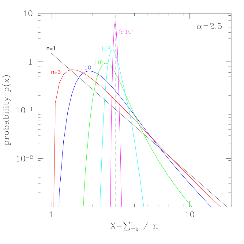
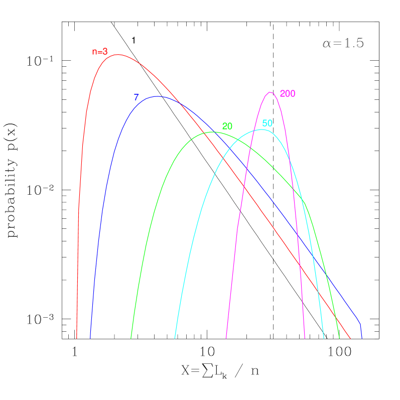
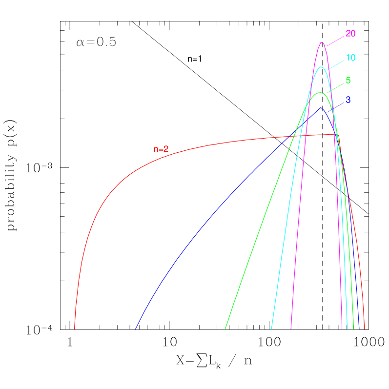
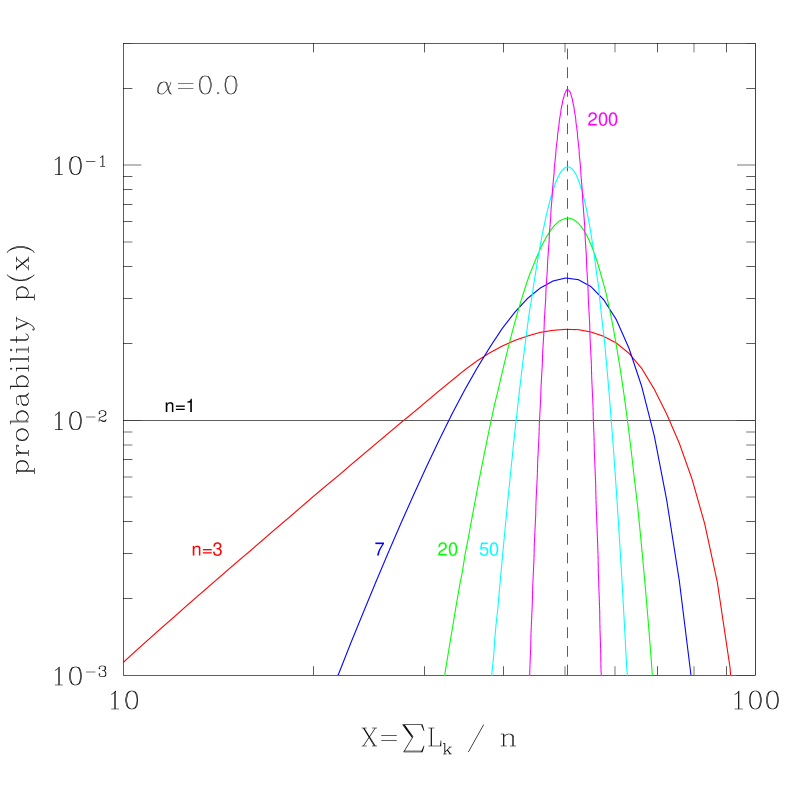
The probability distributions $p_{n}(L_{\rm tot})$ for various values of the slope $\alpha$ and the number of sources $n$ are shown in Fig.1. To facilitate the comparison of distributions for different values of $n$, the abscissa in these plots is the average luminosity $L_{\rm tot}/n=\sum_{k=1}^{k=n}L_{k}/n$. The values of the luminosity cut-offs were fixed at $L_{1}=1$ and $L_{2}=10^{3}$

The skewness of the probability distribution $p_{n}(L_{\rm tot})$ leads to a deviation of its mode $\tilde{L}_{\rm tot}$ (the most probable value of the total luminosity) from the expectation mean $\left<L_{\rm tot}\right>$ indicated in each panel by the vertical dashed line. The effect is most pronounced for $\alpha\sim 3/2$, is unimportant for for shallow luminosity functions with $\alpha<1$ and gradually diminishes with increasing $\alpha$ at $\alpha>2$.

For illustration, we also show in Fig.1 the probability distributions for a flat LF, $\alpha=0$, in which case $\tilde{L}_{\rm tot}$ exactly equals $\left<L_{\rm tot}\right>$. Naturally, for any value of $\alpha$ the $p_{n}(L_{\rm tot})\rightarrow$ Gaussian distribution in the limit of $n\rightarrow\infty$, in accord with the Central Limit Theorem. Correspondingly $\tilde{L}_{\rm tot}\rightarrow\left<L_{\rm tot}\right>$ in this limit.

2.2.2 The most probable value of total luminosity

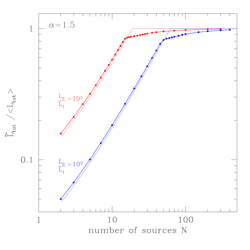
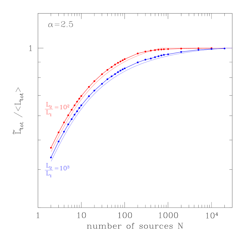
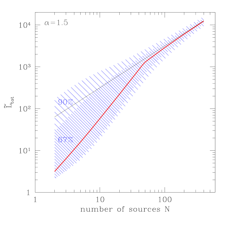
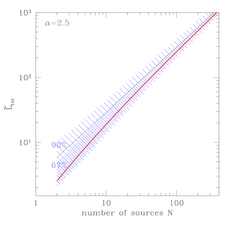
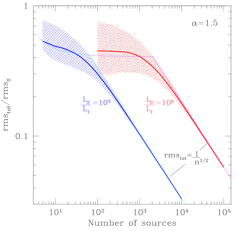
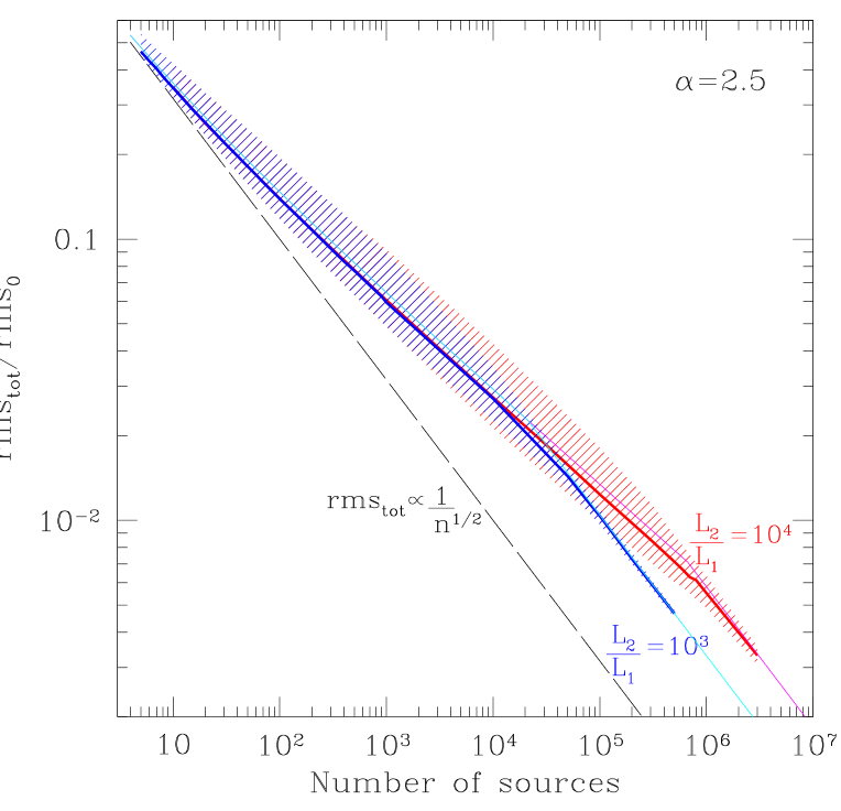
The dependence of the most probable value of the total luminosity $\tilde{L}_{\rm tot}$ on the total number of sources $n$ for different values of $\alpha$ and the ratio $L_{2}/L_{1}$ is shown in Fig.2 and 3. Convenient analytical approximations for the $\tilde{L}_{\rm tot}-n$ relation are derived in Appendix A and its asymptotical behavior is considered in Appendix A.2.

The $\tilde{L}_{\rm tot}-n$ relation is significantly non-linear for “small” number of sources or, equivalently, for small values of the LF normalization $A$. For $L_{1}<<L_{2}$, $\alpha>1$, the boundary between the non-linear and linear regimes, expressed in terms of the normalization $A$, depends only on the LF slope $\alpha$ and its high luminosity cut-off $L_{2}$ (see Appendix A.2). This is due to the fact that the behavior of $\tilde{L}_{\rm tot}$ is defined by the number of sources near the high luminosity cut-off of the luminosity function, rather than by the total number of sources in the entire $L_{1}-L_{2}$ luminosity range, i.e. the condition for the linear regime is:

$$N(L\sim L_{2})\sim L_{2}\frac{dN}{dL}\left(L=L_{2}\right)\ga 1$$ (32)

The total number of sources in the $L_{1}-L_{2}$ luminosity range, on the contrary, is defined by the low luminosity cut-off $L_{1}$ (for $\alpha>1$). For sufficiently large $L_{2}/L_{1}$, the non-linear regime can occur for an arbitrarily large total number of sources (cf. the curves corresponding to different values of $L_{2}/L_{1}$ in Fig.2). Interestingly, for the LF slope in the range of $1<\alpha<2$, where the effect is strongest, there is a relatively sharp break separating the non-linear part of the dependence from the linear part.

Although for small $n$ the most probable value of luminosity $\tilde{L}_{\rm tot}$ can deviate significantly from the expectation mean $\left<L_{\rm tot}\right>$ (Fig.1,2), the condition $\int p\,(L_{\rm tot})\,L_{\rm tot}\,dL_{\rm tot}=\left<L_{\rm tot}\right>$ is satisfied for any $n$. Consequently, the average of $L_{\rm tot}$ over a large number of realizations with the same $n$ always equals $\left<L_{\rm tot}\right>$. This equality is achieved due to the existence of outliers, having values of $L_{\rm tot}$ significantly exceeding both $\tilde{L}_{\rm tot}$ and $\left<L_{\rm tot}\right>$, in accordance with the skewness of the probability distribution $p_{n}(L_{\rm tot})$ for small $n$. This naturally leads to enhanced and asymmetric dispersion of the observed values of $L_{\rm tot}$ in the non-linear regime as illustrated by the shaded areas in Fig.3.

2.3 The luminosity of the brightest source in a sample

The probability distribution for the luminosity of the brightest source observed in a sample of $n$ sources equals:

$$p\,(L_{\rm max})=\left[p_{1}(L<L_{\rm max})\right]^{n-1}p_{1}(L_{\rm max})\ n$$ (33)

where $p_{1}(L)$ is the probability distribution for the luminosity of one source (e.g. eq.(28)) and $p_{1}(L<L_{\rm max})$ denotes the cumulative probability $p_{1}(L<L_{\rm max})=\int_{0}^{L_{\rm max}}p_{1}(L)\,dL$.

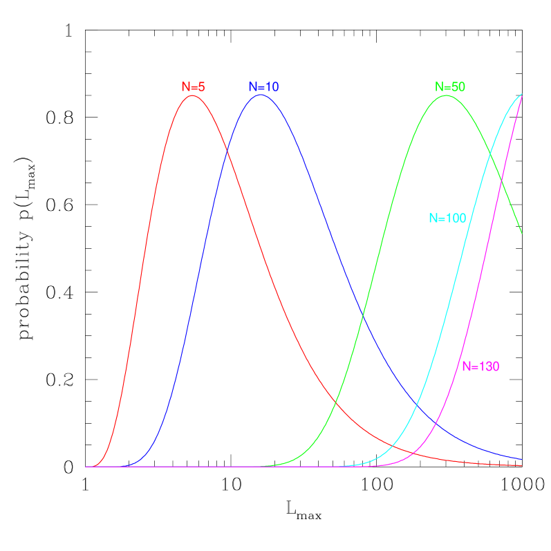
The $p\,(L_{\rm max})$ distribution for $\alpha=1.5$ is shown in Fig.4 and illustrates the intuitively obvious fact that if the number of sources is sufficiently small the brightest sources most likely will not reach the highest possible value of $L_{2}$. An analytical formula for the most probable value of the luminosity of the brightest source is given by eq.(41).

Figure 4: Probability distributions $p\,(L_{\rm max})$ of the luminosity of the brightest source in a sample of $n$ sources with a power law LF with the slope $\alpha=1.5$ and $L_{1}=1$, $L_{2}=10^{3}$. Each curve is marked according to the number of sources $n$.

Figure 5: Variability of the total emission. The ratio of the fractional $rms$ of the combined emission to that of one source, $rms_{0}$, as a function of the number of sources for different values of the LF slope $\alpha$ (indicated in the upper-right corner of each plot) and different values of the ratio of $L_{2}/L_{1}$. The thick solid lines show the square root of the most probable value of the $rms_{\rm\,tot}^{2}/rms_{0}^{2}$, the shaded areas show the 67% intrinsic dispersion, both obtained from the Monte-Carlo simulations. The thin solid lines were computed using the approximation given by eq.(68). The dashed line shows $rms_{\rm\,tot}/rms_{0}\propto 1/\sqrt{n}$ dependence.

3 Variability of the total emission

For a population of $n$ sources with luminosities $L_{k}$ and fractional $rms$ of aperiodic variability $rms_{k}$, the fractional rms of the total emission equals:

$$rms_{\,\rm tot}^{2}=\frac{\sum_{k=1}^{n}L_{k}^{2}\ rms_{k}^{2}}{\left(\sum_{k=1}^{n}L_{k}\right)^{2}}$$ (34)

assuming that variations of the source fluxes are uncorrelated with each other. In the following we also assume for simplicity that all sources have the same value of fractional rms, i.e. $rms_{k}=rms_{0}$.

In the limit of $n\rightarrow\infty$, corresponding to the linear regime in the $\tilde{L}_{\rm tot}-n$ relation, the sums in the eq.(34) can be replaced by the respective integrals of the LF:

$$\frac{rms_{\,\rm tot}^{2}}{rms_{0}^{2}}=\frac{\int L^{2}\,dN/dL\,dL}{\left(\int L\,dN/dL\,dL\right)^{2}}\propto\frac{1}{n}\propto\frac{1}{A}\propto\frac{1}{L_{\rm tot}}$$ (35)

In the linear regime the fractional $rms$ of the collective emission obeys $\propto 1/\sqrt{n}$ averaging law, as expected for uncorrelated variations of individual sources.

In the non-linear regime, however, for a sufficiently flat luminosity function, the total luminosity is defined by a few brightest sources. To first approximation the number of such sources effectively contributing to the sums in eq.(34) does not depend on the LF normalization. Consequently, the fractional $rms$ of the total emission is constant, independently on the total number of sources or of their total luminosity. This contradicts the intuitive expectation that the fractional $rms$ decreases with the number of sources as $rms\propto 1/\sqrt{n}$.

To illustrate this behavior we performed a series of the Monte-Carlo simulations for a power law LF. For each set of parameters and a given value of the number of sources, in each run $n$ sources were placed between $L_{1}$ and $L_{2}$ with a power law luminosity distribution, eq.(31). For each run, the ratio $rms_{\,\rm tot}^{2}/rms_{0}^{2}$ was computed following eq.(34). From results of many runs, the probability distribution for $rms_{\,\rm tot}^{2}/rms_{0}^{2}$ was obtained. The maximum of this distribution defines the most probable value of $rms_{\,\rm tot}^{2}$ and its width characterizes the intrinsic dispersion of this quantity. The examples are shown in Fig.5 for two values of the LF slope, $\alpha=1.5,\,2.5$. For $\alpha<1$ and $\alpha>3$ there is no non-linear regime and the fractional $rms$ of the total emission obeys $\propto 1/\sqrt{n}$ law for any $n$. In plotting Fig.5, we converted $rms_{\,\rm tot}^{2}$ to $rms_{\,\rm tot}$, so that the thick solid curves shows the behavior of the square root of the most probable value of the $rms_{\,\rm tot}^{2}/rms_{0}^{2}$ ratio.

Approximate formulae for $rms_{\,\rm tot}^{2}$ are derived in Appendix B.

Figure 6: Left: The probability distributions $p(L_{\rm tot}/{\rm SFR})$ for different values of SFR. The vertical dashed line shows the expectation mean, defined by eq.(4). Right: The $L_{X}-$SFR relation. The open circles are nearby galaxies observed by Chandra, the filled triangles are spatially unresolved nearby galaxies observed by ASCA and BeppoSAX, for which only total luminosity is available, the filled circles are distant star forming galaxies from the HDF-N. The thick grey line is relation between the SFR and the most probable value of the total luminosity, predicted from the “universal” HMXB XLF, the shaded area shows its 67% intrinsic spread, the dashed line is the expectation mean, defined by eq.(4). The five nearby galaxies, used by Grimm et al. (2003) to derive the “universal” HMXB XLF, are marked as crossed boxes.

4 Astrophysical applications

4.1 Determining LF parameters from total emission of unresolved sources

The shape of the $\tilde{L}_{\rm tot}-A$ relation ($A$ is the normalization of the luminosity function) is defined by the parameters of the luminosity function. For $1\la\alpha\la 2$, it has two distinct power law regimes, separated by a break (Fig.2 and 3):

$$\tilde{L}_{\rm tot}\propto\left\{\begin{array}[]{ll}A^{\frac{1}{\alpha-1}}&A<A_{\rm break}\\ A&A>A_{\rm break}\end{array}\right.$$ (38)

The position of the break between the non-linear and linear regime is defined by the high luminosity cut-off of the LF and its slope as described by eq.(55). This opens a possibility to determine the LF parameters without actually resolving the individual sources, but studying large samples of objects (e.g. galaxies) and the relation between their total emission and the normalization $A$. The value of $A$ in many cases can be determined independently from observations at other wavelengths. For example, the normalizations of the luminosity functions of high and low mass X-ray binaries are proportional to the star formation rate (Grimm et al., 2003) and stellar mass (Gilfanov, 2004) of the host galaxy respectively. Both quantities can be determined from the conventional indicators, such as radio or near-infrared luminosities.

Of course with the sub-arcsec angular resolution of Chandra the luminosity distribution of point sources in nearby galaxies can be studied directly. However, for more distant galaxies, D$\ga 30-50$ Mpc, even Chandra resolution becomes insufficient and only the total luminosity of the galaxy can be measured. Provided that the contaminating contribution of the emission of a central AGN and/or of hot X-ray emitting gas can be constrained or separated, one can study the relation between the total luminosity $L_{X}$ of a (unresolved) galaxy and its star formation rate or stellar mass. The $L_{X}-$SFR or $L_{X}-M_{*}$ “growth curves” constructed for large samples of galaxies and spanning a broad range of SFR and $M_{*}$ can be used to constrain the XLF parameters of X-ray binaries in distant galaxies including those located at intermediate and high redshifts. With this, one can study the influence of a number of factors such as effects of binary evolution, metallicity, regimes of star formation, etc. on the luminosity distribution of X-ray binaries.

4.2 High mass X-ray binaries in star forming galaxies

4.2.1 $L_{X}-$SFR relation for star forming galaxies

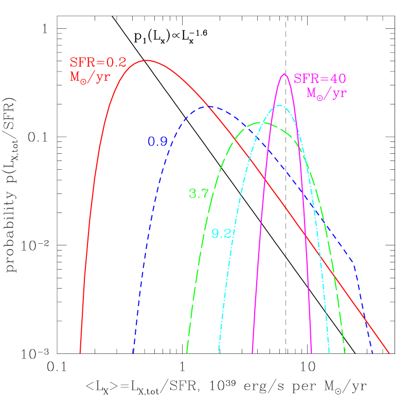
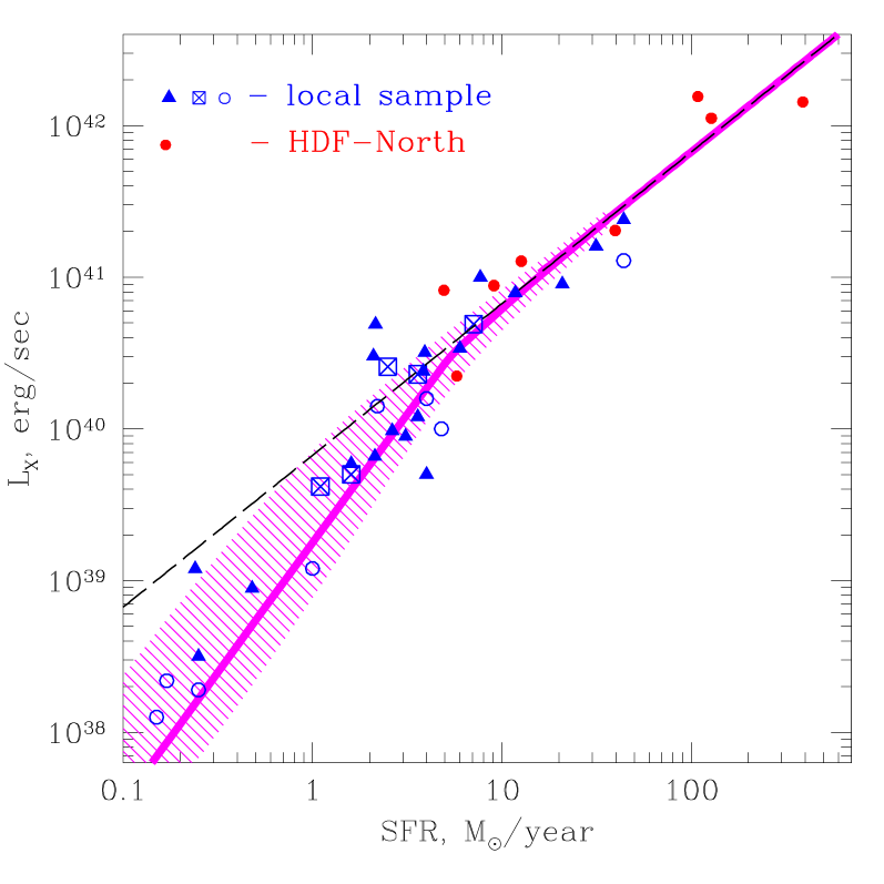
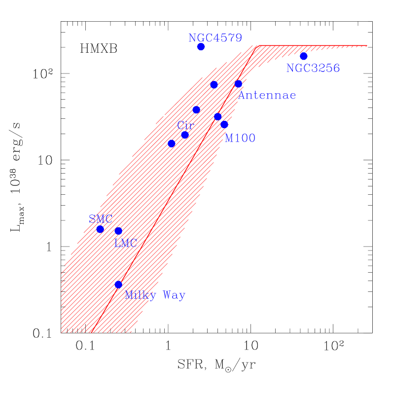
The slope of the “universal” luminosity function of HMXBs, $\alpha=1.6$, is in the range where the non-linear behavior of the $\tilde{L}_{\rm tot}-A$ relation is most pronounced. In the left panel of Fig.6 we plot the probability distribution of the total luminosity $p\,(L_{\rm tot})$, computed for different values of the star formation rate. The distribution is strongly asymmetric in the non-linear low-SFR regime which, for the parameters of the “universal” HMXB XLF, corresponds to the formation rate of massive stars below SFR$\la 4-5$ M_⊙/yr. Note that a small value of SFR does not necessarily imply a small total number of sources, which is defined by the (unknown) low luminosity cut-off of the HMXB XLF. For example, for SFR=0.2 M_⊙/yr, when the non-linear effect is very pronounced, the total number of sources might be as large as $\sim 300$ ($\sim 1200$) for the low luminosity cut-off of $10^{34}$ ($10^{33}$) erg/s. These low values of the star formation rate correspond to the familiar examples of the Milky Way galaxy and the Magellanic Clouds. On the opposite end among the relatively nearby and well known galaxies are the Antennae interacting galaxies which, with the star formation rate of SFR$\sim 7$ M_⊙/yr, have a nearly symmetric $p\,(L_{\rm tot})$ distribution, sufficiently close to the normal distribution.

The predicted $L_{X}-$SFR relation is shown in the right panel in Fig.6, along with the measured values of X-ray luminosities and the star formation rates for a number of nearby galaxies and galaxies observed with Chandra at intermediate redshifts, $z\sim 0.2-1.3$, in the Hubble Deep Field North. The data shown in Fig.6 are from Grimm et al. (2003), complemented with the local galaxies data from Ranalli, Comastri & Seti (2003). In plotting the latter we removed the duplications and the galaxies likely to be contaminated by the contribution of low mass X-ray binaries, unrelated to the current star formation activity, as discussed by Gilfanov et al. (2004). The luminosities and star formation rates for the Hubble Deep Field North galaxies (Brandt et al., 2001) were computed for the following cosmological parameters: $H_{0}=70$ km/s/Mpc, $\Omega_{m}=0.3$, $\Lambda=0.7$, as described in Gilfanov et al. (2004).

Fig.6 further illustrates the difference between the mode and the expectation mean of the $p\,(L_{\rm tot})$ probability distribution. The thick solid line in the right panel shows the SFR–dependence of the mode of $p\,(L_{\rm tot})$ and predicts the most probable value of the X-ray luminosity of a randomly chosen galaxy. If observations of many (different) galaxies with similar values of SFR are performed, the obtained values of $L_{\rm tot}$ will obey the probability distribution depicted in the left panel. The average of the measured values of $L_{\rm tot}$ will be equal to the expectation mean given by eq.(4) and shown by the dashed straight lines in the left and right panels. Due to the properties of $p\,(L_{\rm tot})$ these two quantities are not identical in the low-SFR limit when the total luminosity is defined by the small number of the most luminous sources. Only in the large SFR limit when there are sufficiently many sources with luminosities near the cut-off of the luminosity function, $\log(L_{X})\sim 40$, does the $L_{X}-$SFR relation behave in the intuitively expected way.

Owing to the skewness of the probability distribution $p\,(L_{\rm tot})$ large and asymmetric dispersion among the measured values of $L_{\rm tot}$ is expected in the non-linear low-SFR regime. This asymmetry is already seen in Fig.6 – at low SFR values there are more points above the thick solid curve than below. Moreover, the galaxies lying significantly above the solid and dashed curves in Fig.6 should be expected at low SFR and will inevitably appear as the plot is populated with more objects. Such behavior differs from a typical astrophysical situation and should not be ignored when analyzing and fitting the $L_{X}$–SFR relation in the low SFR regime. In particular, due to non-Gaussianity of the $p\,(L_{\rm tot})$ distribution the standard data analysis techniques – least square and $\chi^{2}$ fitting – become inadequate.

Figure 7: Dependence of the $L_{X}-$SFR relation on the XLF cut-off luminosity $L_{\rm cut}$. The three curves, corresponding to different values of $L_{\rm cut}$ coincide in the non-linear low SFR regime but differ in the position of the break between linear and non-linear regimes. The data are the same as in Fig.6.

Figure 8: Variability of the total emission of HMXBs in star forming galaxies. Dependence of the ratio $rms_{\rm\,tot}/rms_{0}$ on the star formation rate. The thick solid line shows the most probable value of the $rms_{\rm\,tot}/rms_{0}$, the shaded area shows its 67% intrinsic dispersion, both obtained from the Monte-Carlo simulations for a power law LF with the slope of $\alpha=1.6$ and a cut-off at $L_{2}=2\cdot 10^{40}$ erg/s. The dashed line shows asymptotical behavior at large SFR. The filled circles correspond to HMXB sources in the Milky Way, SMC and the Antennae galaxies, computed from eq.(34), using the observed luminosities of X-ray sources in these galaxies.

Figure 9: Left: The probability distribution of the luminosity of the brightest HMXB source for different values of the star formation rate, computed from eq.(33) using the parameters of the “universal” luminosity function of HMXBs. Right: Expected luminosity of the brightest HMXB vs. star formation rate. The thick solid line shows the most probable value of the $L_{\rm max}$ (eq.(41)), the shaded area shows its 67% intrinsic dispersion, obtained from the probability distribution given by eq.(33). The filled circles show maximum observed luminosity of HMXBs in the Milky Way and several nearby star forming galaxies.

4.2.2 High luminosity cut-off in the HMXB XLF

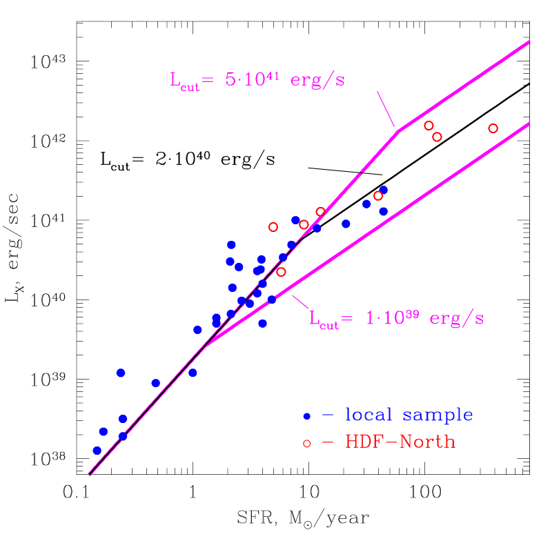
The position of the break between the non-linear and linear parts of the $L_{X}$–SFR relation depends on the LF slope and its cut-off luminosity (Fig.7, eq.55): ${\rm SFR}_{\rm break}\propto L_{\rm cut}^{\alpha-1}$. This allows to constrain the parameters of the luminosity distribution of compact sources using the data of spatially unresolved galaxies as discussed in section 4.1.

Agreement of the predicted $L_{X}-$SFR relation with the data both in high- and low-SFR regimes confirms the universality of the HMXB luminosity function, derived by Grimm et al. (2003) from significantly fewer galaxies (shown as crossed boxes) than plotted in Figs.6, 7. It provides an independent confirmation of the existence of a cut-off in the HMXB XLF at $\log(L_{\rm cut})\sim 40.5$, including HMXBs in spatially unresolved high redshift galaxies from the Hubble Deep Field North. This implies, in particular, that ultra-luminous X-ray sources (ULX) at redshifts of $z\sim 0.2-1.3$ were not significantly more luminous than those observed in the nearby galaxies.

4.2.3 Aperiodic variability

X-ray flux from X-ray binaries is known to be variable in a broad range of time scales, from $\sim$msec to $\sim$ years. In addition to a number of coherent phenomena and quasi-periodic oscillations, significant continuum aperiodic variability is often observed. The fractional rms of aperiodic variations depends on the nature of the binary system and the spectral state of the X-ray source and is usually in the range from a fraction of a per cent to $\sim 20-30$ per cent. Correspondingly, the combined emission of X-ray binaries in a galaxy should be also variable in a similarly broad range of time scales. It has been suggested by Grimm, Gilfanov & Sunyaev (2004) that due to a large difference in the characteristic time scales of the accretion flow onto a stellar mass object and onto a supermassive black hole variability of the X-ray emission from a galaxy can be used to distinguish between the combined emission of a population of X-ray binaries and that of an accreting supermassive black hole in the centre of a galaxy (AGN).

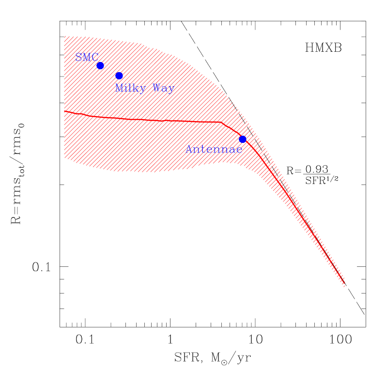
From results of section 3 and Appendix B one should expect that in the non-linear low-SFR regime the fractional $rms$ of the total X-ray emission of a star forming galaxy is independent of SFR. This prediction is confirmed by the results of the Monte-Carlo simulations performed as described in section 3 and shown in Fig.8. For moderate star formation rates, SFR$\la 5-10~{}M_{\sun}$/yr, we predict a rather large aperiodic variability of the total emission of HMXBs at the level of $\sim 1/3-1/2$ of the fractional $rms$ of individual X-ray binaries. At larger values of SFR, corresponding to the linear regime in the $L_{X}-$SFR relation, it decreases as $rms\propto 1/\sqrt{\rm SFR}$, in accord with eq.(68). Also shown in Fig.8 are values of the fractional $rms$ reduction, computed directly from eq.(34) using the luminosities of the observed HMXBs in the Milky Way (Grimm et al., 2002), SMC (Yokogawa et al., 2000), and in the Antennae galaxies (Zezas et al., 2002). Note, that the predicted $rms-$SFR relation can be modified by the luminosity dependence of the $rms$ of individual sources. This factor might become especially important at large values of SFR when the total luminosity of a star forming galaxy is dominated by ULXs whose variability properties we know little about.

Figure 10: Illustration of the effect of hypothetical intermediate mass black holes on the $L_{X}-$SFR relation. Left: The luminosity function of compact sources at different levels of star formation rate. Right: Corresponding $L_{X}-$SFR relation. The thin straight line shows the linear dependence.

4.2.4 Luminosity of the brightest source

As the first Chandra observations of compact sources in nearby galaxies became available, it has been noted (e.g. Sarazin et al., 2001; Irwin et al., 2002; Fabbiano & White, 2003) that the luminosity of the brightest X-ray binary in a galaxy might depend on its properties. In particular in the case of high mass X-ray binaries it appeared to correlate with the star formation rate of the host galaxy. For example, in the Antennae galaxies, a number of compact sources have been discovered with luminosities of $\sim 10^{40}$ erg/s (Zezas et al., 2002). On the other hand, the luminosities of the brightest HMXB sources in the Milky Way do not exceed $\la 10^{38}$ erg/s (Grimm et al., 2002). It has been argued that this might reflect the difference in the intrinsic source properties, related to the difference in the galactic environment and in initial conditions for X-ray binary formation in starburst galaxies and in galaxies with weak and steady star formation.

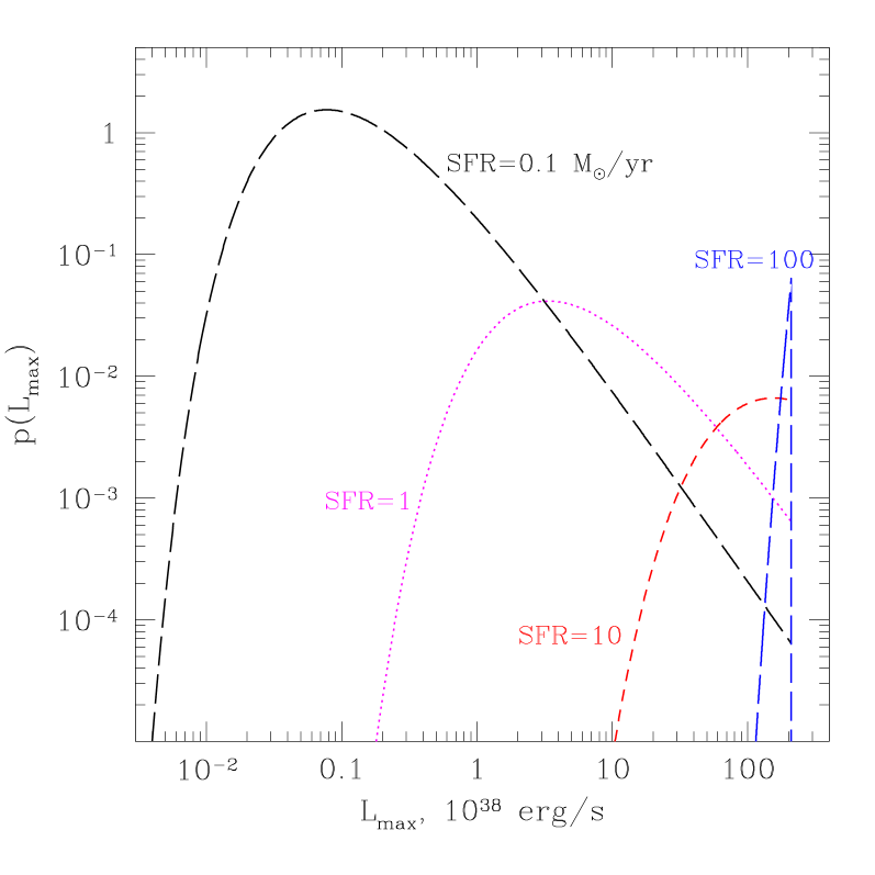
However, as discussed in section 2.3, the probability distribution for the luminosity of the brightest source in a galaxy, $p\,(L_{\rm max})$, depends on the LF normalization, i.e. on the SFR of the host galaxy in the case of HMXBs. The luminosity of the brightest source increases with SFR, until it reaches the maximum possible value, defined by the high luminosity cut-off of the LF. The $p\,(L_{\rm max})$ distributions, computed from eq.(33) for the parameters of the “universal” HMXB XLF, are shown for different values of SFR in the left panel of Fig.9. The right panel in Fig.9 shows the dependence of the most probable value of the luminosity of the brightest HMXB on the SFR of the host galaxy, described by eq.(41), along with its intrinsic 67% uncertainty. Filled symbols in Fig.9 are the luminosities of the brightest source observed in star forming galaxies from the sample of Grimm et al. (2003, and references therein). As is clear from the plot, the large difference in the maximum luminosity between low- and high-SFR galaxies, e.g. between the Milky Way and the Antennae galaxies, can be naturally understood in terms of the properties of the probability distribution $p\,(L_{\rm max})$. No additional physical processes, affecting HMXBs formation in starburst galaxies, need to be invoked.

4.3 Intermediate mass black holes

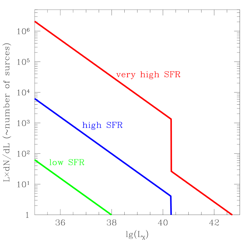
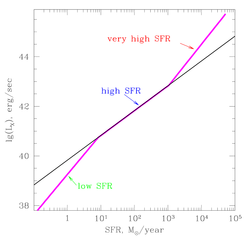
The hypothetical intermediate mass black holes, probably reaching masses of $\sim 10^{2-5}M_{\odot}$, might be produced, e.g. via black hole merges in dense stellar clusters, and can be associated with extremely high star formation rates. To accrete efficiently they should form close binary systems with normal stars or be located in dense molecular clouds. It is natural to expect, that such objects are significantly less frequent than $\sim$stellar mass black holes. The transition from $\sim$stellar mass BH HMXB to intermediate mass BHs should manifest itself as a step in the luminosity distribution of compact sources (Fig.10, left panel). If the cut-off in the HMXB XLF, observed at $\log(L_{\rm cut})\sim 40.5$ corresponds to the maximum possible luminosity of “ordinary” $\sim$stellar mass black holes and if at $L>L_{\rm cut}$ a population of hypothetical intermediate mass BHs emerges, it should lead to a drastic change in the slope of the $L_{X}$–SFR relation at extreme values of SFR (Fig.10, right panel). Therefore, observations of $L_{X}-$SFR relation for distant star forming galaxies with very high SFR might be an easy way to probe the population of intermediate mass black holes.

Figure 11: Left: Probability distribution for the luminosity of the brightest LMXB for different values of the stellar mass, computed from eq.(33), using the parameters of the broken power law approximation to the “universal” luminosity function of LMXBs. Right: Expected luminosity of the brightest LMXB source vs. stellar mass of the host galaxy. The thick solid line shows the most probable value of the $L_{\rm max}$, the shaded area shows its 67% intrinsic dispersion, both obtained from the probability distribution given by eq.(33). The filled circles show maximum observed luminosities of LMXB sources in the Milky Way and several nearby galaxies, studied with Chandra. The “broken” shape of the predicted dependence is a consequence of the broken power law approximation of the “universal” LMXB XLF, used in the calculations.

4.4 Low mass X-ray binaries

4.4.1 $L_{X}-$stellar mass relation and maximum luminosity

As was shown by Gilfanov (2004) the luminosity distribution of low mass X-ray binaries in nearby early type galaxies and bulges of spiral galaxies can be described by a “universal” XLF whose shape is approximately the same in different galaxies and whose normalization is proportional to the stellar mass of a galaxy. The shape of the “universal” LMXB XLF is significantly more complex than that of HMXBs. It appears to follow the $L^{-1}$ power law at low luminosities, gradually steepens at $\log(L_{X})\ga 37.0-37.5$, and has a rather abrupt cut-off at $\log(L_{X})\sim 39.0-39.5$. In the $\log(L_{X})\sim 37.5-38.7$ luminosity range, it approximately follows a power law with the differential slope of $\approx 1.8-1.9$.

Given the shape of the XLF, the total luminosity of LMXB sources in a galaxy is defined by the sources with $\log(L_{X})\sim 37-38$, the contribution of the brighter and, especially, weaker sources being less significant. Therefore the non-linear regime in the $L_{X}-M_{*}$ relation, although does exist for $\log(M_{*})\la 10.0-10.5$, is less important than in the $L_{X}-$SFR relation for high mass X-ray binaries (see, for example, Fig.14 in Gilfanov 2004).

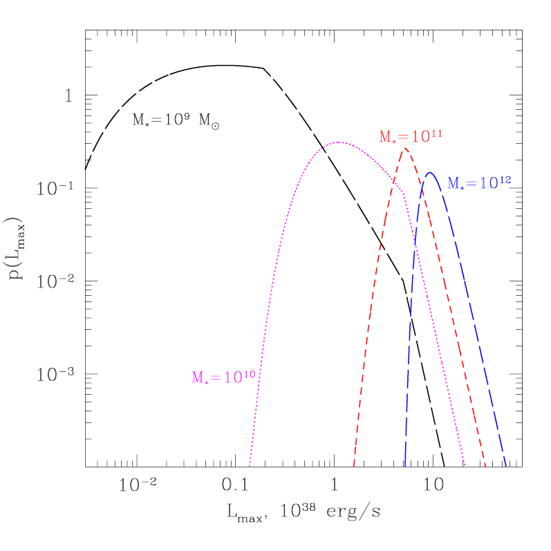
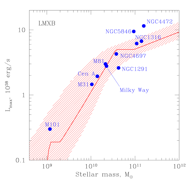
Significantly more pronounced is the dependence of the luminosity of the brightest source on the LF normalization, i.e. on the stellar mass of the host galaxy. In order to study this dependence we used the broken power law approximation for the LMXB XLF from Gilfanov (2004) and performed a series of the Monte-Carlo simulations, similar to those described in section 3. The probability distribution of the maximum luminosity $p\,(L_{\rm max})$, obtained from these simulations, is shown in the left panel in Fig.11 for different values of the stellar mass of the host galaxy. The right panel shows the dependence of the most probable value of the maximum luminosity and of its 67% intrinsic spread on the stellar mass. Its broken line shape is a result of the broken power law approximation of the LMXB XLF used in the simulations. Solid symbols show the observed values of the maximum luminosity for the number of nearby early type galaxies, bulges of spiral galaxies and for LMXBs in the Milky Way from the sample of Gilfanov (2004, and references therein).

Similarly to HMXBs in star forming galaxies it is obvious from Fig.11 that the significant difference in the value of the luminosity of the brightest source can be naturally explained by the properties of the luminosity function of LMXBs. The same effect leads to an artificial (unphysical) dependence of the average luminosity of low mass X-ray binaries in a galaxy on its stellar mass (e.g. Fig.17 in Gilfanov 2004). So far there is no evidence for a significant change of intrinsic properties of low mass X-ray binaries with galactic environment. The difference between the luminosity of the brightest LMXB in massive elliptical galaxies and the bulges of spiral galaxies can be understood based on the probability arguments.

4.4.2 Variability

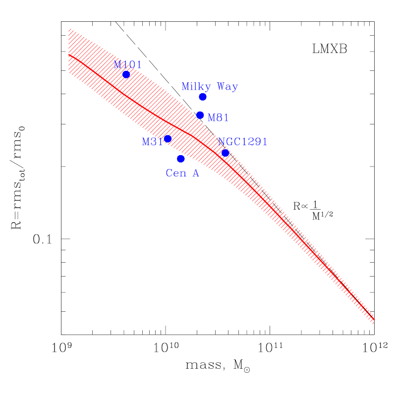
As in the case of HMXBs, in the linear large-mass limit, $\log(M_{*})\ga 10.5$, the fractional $rms$ of the aperiodic variability of the combined emission of LMXBs follows the $rms_{\rm\,tot}\propto 1/\sqrt{M_{*}}$ averaging law. Owing to the shape of the LMXB XLF it decreases rather quickly with the stellar mass of the galaxy in the non-linear low-mass regime as well (Fig.12). Consequently, in massive elliptical galaxies, with stellar mass $\log(M_{*})\sim 11.0-11.5$, the fractional $rms$ variability of the total emission will be suppressed by a factor of $\sim 10-15$ with respect to the $rms$ of individual sources. In a galaxy similar to the Milky Way with $\log(M_{*})\sim 10.5-10.7$ the suppression factor is $\sim 5$. Considerable variability on the level of $\sim 1/4-1/2$ of that of individual X-ray binaries can be expected only for light bulges of spiral galaxies with masses in the $\log(M_{*})\sim 9.5-10.5$ range.

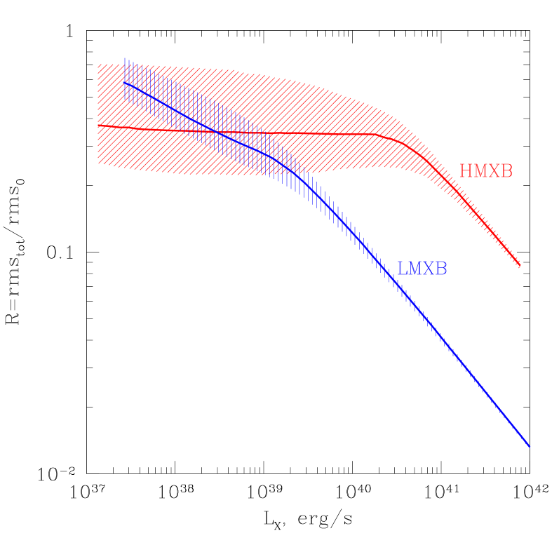
Fig.13 compares the dependence of the fractional $rms$ on the most probable value of the total luminosity for high and low mass X-ray binaries. In the bright luminosity end, $\log(L_{X})\ga 39.5$, the X-ray emission from early type galaxies is expected to be significantly, up to a factor of $\sim 7$, less variable than from star forming galaxies.

Figure 12: Variability of the total emission of low mass X-ray binaries. Dependence of the ratio $rms_{\rm\,tot}/rms_{0}$ on the stellar mass of the galaxy. The thick solid line shows the most probable value of the $rms_{\rm\,tot}/rms_{0}$, the shaded area shows its 67% intrinsic dispersion, both obtained from the Monte-Carlo simulations for the “universal” luminosity function from Gilfanov (2004). The dashed line shows asymptotical behavior at large $M_{*}$. The filled circles correspond to LMXBs in the Milky Way and several nearby galaxies, computed from eq.(34), using the observed luminosities of X-ray sources in these galaxies.

Figure 13: Comparison of variability of low and high mass X-ray binaries. Dependence of the ratio $rms_{\rm\,tot}/rms_{0}$ on the total X-ray luminosity of the galaxy due to X-ray binaries. The thick solid lines show the most probable value of the $rms_{\rm\,tot}/rms_{0}$, the shaded areas show its 67% intrinsic dispersion, both obtained from the Monte-Carlo simulations for the respective “universal” luminosity functions from Grimm et al. (2003) and Gilfanov (2004). For both curves, the linear parts at high $L_{X}$ follow $rms\propto 1/\sqrt{L_{X}}$ averaging law.

5 Summary

We studied the statistical properties of the combined emission of a population of discrete sources. Namely, we considered the properties of their total luminosity

$$L_{\rm tot}=\sum_{k=1}^{k=n}L_{k}$$ (39)

and its dependence on the number of sources $n$ or, equivalently, on the normalization of the luminosity function (LF). Using high mass X-ray binaries in star forming galaxies as an example, $L_{k}$ are the luminosities of individual X-ray binaries in a galaxy and $L_{\rm tot}$ is its total X-ray luminosity due to HMXB population. In this example the normalization of the luminosity function, i.e. the number of HMXBs in the galaxy $n$, is proportional to its star formation rate. We showed that due to statistical properties of the probability distribution $p\,(L_{\rm tot})$ the result of a measurement of the total luminosity of a randomly chosen galaxy might deviate significantly from the intuitively obvious expression

$$\left<L_{\rm tot}\right>=\int_{0}^{+\infty}L\,\frac{dN}{dL}\,dL\propto n\propto{\rm SFR}$$ (40)

These properties of $p\,(L_{\rm tot})$ can result in a surprising non-linear dependence of the total luminosity on $n$. They can also cause anomalous variability of the combined emission in an apparent violation of the $rms\propto 1/\sqrt{n}\,$ averaging law for uncorrelated variations of individual sources.

Our results can be summarized as follows:

1. The probability distribution $p\,(L_{\rm tot})$ can be computed numerically from eq.(24) or alternatively eq.(27). Examples are shown in Fig.1.

2. The relevant characteristics of the $p\,(L_{\rm tot})$ distribution are: (1) its mode $\tilde{L}_{\rm tot}$ – the value of the random variable $L_{\rm tot}$ for which $p\,(L_{\rm tot})$ has the maximum and (2) the expectation mean $\left<L_{\rm tot}\right>$ defined by eq.(40).

   It is the mode of the $p\,(L_{\rm tot})$ distribution that predicts the most probable value of the total luminosity of a randomly chosen galaxy. If many galaxies with $\sim$same total number of sources $n$ are observed the measured values of their total X-ray luminosities are distributed according to the $p\,(L_{\rm tot})$ distribution whose shape depends on the chosen value of $n$ (Fig.6, left panel). The average of the measured values of $L_{\rm tot}$ is equal to the expectation mean $\left<L_{\rm tot}\right>$ and is always proportional to $n$ in agreement with eq.(40).

3. For small values of the LF normalization, $\tilde{L}_{\rm tot}$ and $\left<L_{\rm tot}\right>$ do not equal each other (Fig.1) and the $\tilde{L}_{\rm tot}-n$ relation is non-linear (Fig.2–3, 6). Only in the limit of $n\gg 1$, $\tilde{L}_{\rm tot}=\left<L_{\rm tot}\right>$ and $\tilde{L}_{\rm tot}$ depends on $n$ linearly. The threshold value of $n$ depends on the LF shape and can be arbitrarily large.

4. The skewness of the $p\,(L_{\rm tot})$ probability distribution in the non-linear regime (Fig.1) results in an enhanced and significantly asymmetric intrinsic dispersion of the measured values of $L_{\rm tot}$ (Fig.3,6). Its non-Gaussianity precludes the use of the standard fitting techniques in analyzing the $L_{\rm tot}-n$ relation (e.g. $L_{X}-$SFR relation for star forming galaxies), such as $\chi^{2}$ minimization technique.

5. The variability of the total emission (e.g. aperiodic variability of X-ray emission of a galaxy due to superposition of variabilities of individual sources) in the non-linear regime decreases with the number of sources more slowly than $rms\propto 1/\sqrt{n}\,$ law for uncorrelated variations of individual sources, resulting in anomalously high variability of the total emission. In the linear regime the $rms\propto 1/\sqrt{n}$ dependence is restored (section 3, Fig.5).

6. The amplitude of the discussed effect depends on the shape of the luminosity function. For a power law LF it is strongest for $1<\alpha<2$, is unimportant for shallow luminosity functions with $\alpha<1$, and gradually diminishes with increase of $\alpha$ above $\alpha=2$ (Fig.1–3).

We illustrate these results using the example of the combined emission of X-ray binaries in galaxies and its dependence on the star formation rate and on the stellar mass of the host galaxy.

1. For the slope of the HMXB “universal” XLF, $\alpha\approx 1.6$, the discussed effects are strongest with a significant non-linear regime in the $L_{X}-$SFR relation at SFR$\la 4-5$ $M_{\odot}$/yr. The predicted $L_{X}-$SFR dependence is in good agreement with observations (Fig.6). Given the shape of the “universal” LMXB XLF no significant non-linearity of the $L_{X}-M_{*}$ relations is expected, also in a good agreement with observations.

2. The $L_{X}-$SFR relation can be used to constrain the XLF parameters of HMXBs in distant unresolved galaxies including the galaxies observed with Chandra in HDF-N at redshifts $z\sim 0.2-1.3$ (sections 4.2.2, 4.3, Figs.7, 10).

3. Both for high and low mass X-ray binaries a strong dependence of the luminosity of the brightest source on the SFR and stellar mass of the host galaxy is expected. The $L_{\rm max}-$SFR and $L_{\rm max}-M_{*}$ dependences predicted from the respective “universal” XLFs explain well the results of Chandra observations of nearby galaxies (Fig.9 and 11). The significant difference in the luminosity of the brightest LMXB between bulges of spiral galaxies and giant ellipticals or between the brightest HMXB in the Milky Way and in starburst galaxies can be understood based solely on probability arguments.

4. We predict enhanced variability of X-ray emission from star forming galaxies due to HMXBs, significantly above the $\propto 1/\sqrt{n}$ averaging law. For SFR$\la 5$ M_⊙/yr the expected fractional $rms$ of variability of the combined emission of HMXBs does not depend on the star formation rate and approximately equals  $\sim 1/3-1/2$ of the $rms$ of individual sources (Fig.8). On the contrary, variability of X-ray emission from early type galaxies due to LMXBs will be significantly suppressed because of the averaging effect (Fig.12), upto $\sim 3-10$ times in the $\sim 10^{10}-10^{11}$ M_⊙ stellar mass range. For the same total luminosity star forming galaxies are expected to have significantly larger fractional $rms$, than massive elliptical and S0 galaxies assuming that fractional the $rms$ of individual sources are comparable (Fig.13).

6 Acknowledgements

We thank the anonymous referee for the comments, which helped to improve the presentation of the paper.

Appendix A Approximate solution for the total luminosity

We consider the case of a power law LF, eq.(31), with a slope $\alpha>0$. The probability distribution for the luminosity of the brightest source in the sample of $n$ sources is defined by eq.(33). The maximum of this distribution gives the most probable value of the luminosity of the brightest sources:

$$\tilde{L}_{\rm max}=\min\left(L^{\prime}_{\rm max}\,,L_{2}\right)$$ (41)

$$\left(\frac{L^{\prime}_{\rm max}}{L_{1}}\right)^{\alpha-1}=1+\frac{\alpha-1}{\alpha}\,(n-1)$$

Similarly, the probability distribution of the minimum luminosity in the sample is:

$$p\,(L_{\rm min})=\left[p_{1}(L>L_{\rm min})\right]^{n-1}p_{1}(L_{\rm min})\ n$$ (42)

Contrary to $p\,(L_{\rm max})$ $p\,(L_{\rm min})$ declines steeply at $L>L_{1}$ for any $n$ (for $\alpha>0$). Within the accuracy of this approximation we can assume $p\,(L_{\rm min})=\delta(L_{\rm min}-L_{1})$, i.e. $L_{\rm min}=L_{1}$.

The total luminosity of $n$ sources distributed between $L_{1}$ and $L_{\rm max}$ according to the power law with the slope of $\alpha$ ($\alpha\neq 1,\ \alpha\neq 2$) can be approximated as:

$$L_{\rm tot}\approx n\;\frac{1-\alpha}{2-\alpha}\;\frac{L_{\rm max}^{2-\alpha}-L_{1}^{2-\alpha}}{L_{\rm max}^{1-\alpha}-L_{1}^{1-\alpha}}$$ (43)

Knowing the probability distribution $p\,(L_{\rm max})$ the probability distribution $p_{n}(L_{\rm tot})$ can be calculated as:

$$p_{n}(L_{\rm tot})\approx p\,(L_{\rm max})\cdot\left(\frac{dL_{\rm tot}}{dL_{\rm max}}\right)^{-1}$$ (44)

where $L_{\rm max}=L_{\rm max}(L_{\rm tot})$ is inverse function to eq.(43) and $p\,(L_{\rm max})$ is given by eq.(33).

The most probable value of $L_{\rm tot}$ is defined by the condition

$$\frac{dp_{n}(L_{\rm tot})}{dL_{\rm tot}}=0$$ (45)

With eq.(33), (43) and (44) the above equation can be transformed to:

$$(\alpha-2)\xi^{2\alpha}-(\alpha-2)(1+\alpha-n+\alpha n)\xi^{1+\alpha}+$$ (46)

$$+(\alpha-1)^{2}(1+n)\xi^{\alpha}+\left[1+(\alpha-1)n\right]\xi^{2}=0$$

$$\xi=\frac{L_{\rm max}}{L_{1}}$$

or, equivalently:

$$n=\frac{(\alpha-2)\xi^{2\alpha}+(2+\alpha-\alpha^{2})\xi^{1+\alpha}+(\alpha-1)^{2}\xi^{\alpha}-\xi^{2}}{(\alpha-1)[(\alpha-2)\xi^{1+\alpha}-(\alpha-1)\xi^{\alpha}+\xi^{2}]}$$ (47)

$\alpha\neq 1,\ \alpha\neq 2$. Because of the simplifying assumption $p_{\rm min}(L_{\rm min})=\delta(L_{\rm min}-L_{1})$ and the approximate nature of eq.(43), the probability distribution defined by eq.(44), is valid only for $L_{\rm tot}<\left<L_{\rm tot}\right>$ and is undefined otherwise. This, however, is sufficient for our purpose as $L_{\rm max}\sim L_{2}$ corresponds to the break in the $\tilde{L}_{\rm tot}-n$ relation (Fig.2 and 3), above which $\tilde{L}_{\rm tot}=\left<L_{\rm tot}\right>$.

A.1 The practical recipe

The $\tilde{L}_{\rm tot}-n$ relation can be computed parametrically using eqs.(47) and (43) The practical recipe is for a set of values of $L_{\rm max}$, $L_{1}<L_{\rm max}\leq L_{2}$, to compute $n$ from eq.(47) and $L_{\rm tot}$ from eq.(43). The pairs of values $(L_{\rm tot},n)$ define the $\tilde{L}_{\rm tot}-n$ relation before and up to the break. Above the break, $\tilde{L}_{\rm tot}=\left<L_{\rm tot}\right>$ and can be computed from eq.(43) with $L_{\rm max}=L_{2}$ and $n>n_{\rm break}$ – free parameter. The $n$ in the obtained $\tilde{L}_{\rm tot}-n$ relation can be transformed to the normalization $A$ via eq.(15).

The approximation defined by the eqs.(47) and (43) is compared with the results of the exact calculation in Fig.2. It is accurate within $\sim$ several per cent everywhere, except the break region, where its accuracy is $\sim 10-20\%$.

A.2 Asymptotics

Using the approximate solution for $\tilde{L}_{\rm tot}$ from Appendix A we consider the asymptotical behavior of the $\tilde{L}_{\rm tot}-n$ relation in the limit of $L_{2}/L_{1}\rightarrow\infty$, $\alpha>1$.

From eq.(47) variable $\xi$ is related to the number of sources by (see footnote 2):

$$\xi^{\alpha-1}=(\alpha-1)n+O(1)$$

$$L_{\rm max}=\xi L_{1}$$ (48)

in the limit of $n>>1$ or equivalently $L_{\rm max}>>L_{1}$. Although in the limit $n\rightarrow\infty$ this approximation is valid for any $\alpha>1$, its accuracy deteriorates considerably for $\alpha\la 1.6$ where it can be improved by replacing $n$ in eq.(48):

$$n\rightarrow n-\frac{1+\alpha-\alpha^{2}}{(\alpha-1)(\alpha-2)},~{}~{}1<\alpha\la 1.6$$ (49)

The most probable value of the total luminosity is given by

$$\frac{\tilde{L}_{\rm tot}}{\left<L_{\rm tot}\right>}\approx\frac{1-\left[(\alpha-1)\,n\,\right]^{\frac{2-\alpha}{\alpha-1}}}{1-\left(L_{2}/L_{1}\right)^{2-\alpha}}$$ (50)

$\alpha>1$, $\alpha\neq 2$, $n>>1$. Using eq.(15), (16) it can be expressed via the normalization of the luminosity function $A$ or transformed to the relations for $\tilde{L}_{\rm tot}$. As with eq.(48), the accuracy of eq.(50) can be significantly improved using eq.(49) for $\alpha\la 1.6$.

For $1<\alpha<2$ the $\tilde{L}_{\rm tot}-n$ relation shows a sharp break between the non-linear and linear regimes (Fig.2,3). From eq.(50) one can obtain:

$$\tilde{L}_{\rm tot}\propto\left\{\begin{array}[]{ll}n^{\frac{1}{\alpha-1}}&n<n_{\rm break}\\ n&n>n_{\rm break}\end{array}\right.$$ (53)

This is in an agreement with eq.(12) based on simple qualitative arguments. The position of the break in the $\tilde{L}_{\rm tot}-n$ relation can be obtained from eq.(47) substituting $\xi=\frac{L_{2}}{L_{1}}$ and using the fact that $\xi>>1$:

$$n_{\rm break}\approx\frac{1}{\alpha-1}\cdot\left(\frac{L_{2}}{L_{1}}\right)^{\alpha-1}$$ (54)

Expressed in terms of the the normalization $A$ of the luminosity function eq.(31) it is:

$$A_{\rm break}\approx L_{2}^{\alpha-1}$$ (55)

As intuitively expected, the break position expressed in terms of the normalization of the luminosity function does not depend on the low luminosity cut-off $L_{1}$ and is defined only by the slope of the luminosity function and the high luminosity cut-off (see discussion in section 2.2.2). The total luminosity at the break, however, depends on the low luminosity cut-off for steep luminosity function with $\alpha>2$:

$$L_{\rm tot,break}\approx\left\{\begin{array}[]{ll}\frac{L_{2}}{2-\alpha}&\mbox{if $1<\alpha<2$}\\ \frac{L_{2}}{\alpha-2}\times\left(\frac{L_{2}}{L_{1}}\right)^{\alpha-2}&\mbox{if $\alpha>2$}\end{array}\right.$$ (58)

as the total luminosity for $\alpha>2$ is defined by the sources near the low luminosity cut-off.

Appendix B Variability of the total emission

In the linear regime of $L_{\rm tot}-n$ relation, the fractional $rms^{2}$ of the collective emission is inversely proportional to the number of sources:

$$\frac{rms_{\,\rm tot}^{2}}{rms_{0}^{2}}\approx\left\{\begin{array}[]{ll}\frac{(2-\alpha)^{2}}{(1-\alpha)(3-\alpha)}\ \frac{1}{n}&\mbox{if $\alpha<1$}\\ \frac{(2-\alpha)^{2}}{(\alpha-1)(3-\alpha)}\ \left(\frac{L_{2}}{L_{1}}\right)^{\alpha-1}\frac{1}{n}&\mbox{if $1<\alpha<2$}\\ \frac{(2-\alpha)^{2}}{(\alpha-1)(3-\alpha)}\ \left(\frac{L_{2}}{L_{1}}\right)^{3-\alpha}\frac{1}{n}&\mbox{if $2<\alpha<3$}\\ \frac{(2-\alpha)^{2}}{(\alpha-1)(\alpha-3)}\ \frac{1}{n}&\mbox{if $\alpha>3$}\end{array}\right.$$ (63)

or, equivalently, to their total luminosity:

$$\frac{rms_{\,\rm tot}^{2}}{rms_{0}^{2}}\approx\left\{\begin{array}[]{ll}\frac{2-\alpha}{3-\alpha}\ \frac{L_{2}}{L_{\rm tot}}&\mbox{if $\alpha<2$}\\ \frac{\alpha-2}{3-\alpha}\ \frac{L_{2}}{L_{\rm tot}}\ \left(\frac{L_{1}}{L_{2}}\right)^{\alpha-2}&\mbox{if $2<\alpha<3$}\\ \frac{\alpha-2}{\alpha-3}\ \frac{L_{1}}{L_{\rm tot}}&\mbox{if $\alpha>3$}\end{array}\right.$$ (67)

The above formulae are valid in the limit $L_{1}<<L_{2}$.

Similarly to the most probable value of the total luminosity (Appendix A) the fractional $rms$ of the total emission can be approximately calculated substituting $L_{2}$ in eq.(35) with some value $L_{\rm max}\leq L_{2}$. In principle, the probability distribution for the $rms_{\rm\,tot}$ in eq.(34) could be derived using the probability distribution for $L_{\rm max}$. The maximum of this probability distribution would give a sufficiently accurate approximation for $rms_{\,\rm tot}/rms_{0}$. However, for simplicity we use the value of $L_{\rm max}$ from eq.(47). In the limit $L_{2}>>L_{1}$ one finds for $1<\alpha<3$:

$$\frac{rms_{\,\rm tot}^{2}}{rms_{0}^{2}}=\frac{(\alpha-2)^{2}}{(\alpha-1)(3-\alpha)}\,\frac{\xi^{3-\alpha}}{(\xi^{2-\alpha}-1)^{2}}\,\frac{1}{n}$$ (68)

for $n<n_{\rm break}$, where $\xi$ is defined by eq.(48) with substitution of eq.(49) for $1<\alpha\la 1.6$ and $n_{\rm break}$ is defined by eq.(54). For $\alpha<1$ and $\alpha>3$ there is no non-linear regime and the fractional $rms_{\rm tot}$ obeys eq.(63) and (67) for any $n$.

From eq.(68) one finds for $1<\alpha<2$

$$\frac{rms_{\,\rm tot}^{2}}{rms_{0}^{2}}=\frac{(\alpha-2)^{2}}{(3-\alpha)}\ \ \ \ \ \ \ \ \ \ n<n_{\rm break}$$ (69)

i.e. in the non-linear regime the fractional $rms$ of the collective emission does not depend on the number of sources.

The accuracy of eqs.(68) and (69) is sufficiently good for $\alpha\ga 1.5$ but deteriorates for smaller values of $\alpha$. In the linear regime eqs.(63) and (67) are almost precise, their only approximation is in neglecting higher orders of the $L_{1}/L_{2}$.

References

- Brandt et al. (2001) Brandt W.N. et al., 2001, AJ, 122, 2810
- Cervino & Luridana (2004) Cervino M. & Luridana V., 2004, A&A, 413, 145
- Fabbiano & White (2003) Fabbiano G. & White N., 2003, in: “Compact Stellar X-ray Sources”, Cambridge University Press (eds., W. Lewin & M. van der Klis), astro-ph/0307077
- Gilfanov (2004) Gilfanov M., 2004, MNRAS, in press, astro-ph/0309454
- Gilfanov et al. (2004) Gilfanov M., Grimm H.-J. & Sunyaev R., 2004, MNRAS, 347, L57
- Grimm et al. (2002) Grimm H.-J., Gilfanov M.& Sunyaev R., 2002, A&A, 391, 923
- Grimm et al. (2003) Grimm H.-J., Gilfanov M.& Sunyaev R., 2003, MNRAS, 339, 793
- Grimm et al. (2004) Grimm H.-J., Gilfanov M.& Sunyaev R., 2004, in preparation
- (9) Illarionov A.F. & Sunyaev R.A., A&A, 1975, 39, 185
- Irwin et al. (2002) Irwin J.A., Sarazin C.L. & Bregman J.N., 2003, ApJ, 570, 152
- Kalogera et al. (2001) Kalogera V. et al, ApJ, 2001, 556, 340
- Ranalli et al. (2003) Ranalli P., Comastri A. & Seti G., 2003, A&A, 399, 39
- Sarazin et al. ( 2001) Sarazin C.L., Irwin J.A.& Bregman J.N, 2001, ApJ, 556, 533
- Shtykovskii & Gilfanov (2004) Shtykovskii P. & Gilfanov M., in preparation
- Yokogawa et al. (2000) Yokogawa J. et al., 2000, ApJS, 128, 491
- Zezas et al. (2002) Zesas A. et al., 2002, ApJS, 142, 239