Photometric redshifts with the $Multilayer$ $Perceptron$ Neural Network: application to the HDF–S and SDSS

We present a technique for the estimation of photometric redshifts based on feed-forward neural networks. The Multilayer Perceptron (MLP) Artificial Neural Network is used to predict photometric redshifts in the HDF–S from an ultra deep multicolor catalog. Various possible approaches for the training of the neural network are explored, including the deepest and most complete spectroscopic redshift catalog currently available (the Hubble Deep Field North dataset) and models of the spectral energy distribution of galaxies available in the literature. The MLP can be trained on observed data, theoretical data and mixed samples. The prediction of the method is tested on the spectroscopic sample in the HDF–S (44 galaxies). Over the entire redshift range, $0.1<z<3.5$, the agreement between the photometric and spectroscopic redshifts in the HDF–S is good: the training on mixed data produces $\sigma_{z}^{test}\simeq 0.11$, showing that model libraries together with observed data provide a sufficiently complete description of the galaxy population. The neural system capability is also tested in a low redshift regime, $0<z<0.4$, using the Sloan Digital Sky Survey Data Release One (DR1) spectroscopic sample. The resulting accuracy on 88108 galaxies is $\sigma_{z}^{test}\simeq 0.022$. Inputs other than galaxy colors - such as morphology, angular size and surface brightness - may be easily incorporated in the neural network technique. An important feature, in view of the application of the technique to large databases, is the computational speed: in the evaluation phase, redshifts of $10^{5}$ galaxies are estimated in few seconds.

1 Introduction

Deep multicolor surveys, using a selection of broad- and/or intermediate-band filters to simultaneously cover the spectral energy distribution (SED) of a large number of targets, have been an important part of astronomy for many years but have remarkably surged in popularity in recent times. Digital detectors and telescopes with improved spatial resolution in all wavelength regimes have enabled astronomers to reach limits that were unthinkable only a few decades ago and are now revealing extremely faint sources (see for a review Cristiani, Renzini & Williams 2001). A general hindrance for the transformation of this wealth of data into cosmologically useful information is the difficulty in obtaining spectroscopic redshifts of faint objects, which, even with the new generation of 8m-class telescopes, is typically limited to I(AB)$\simeq$25. This has spurred a widespread interest in the estimation of the redshift directly from the photometry of the targets (photometric redshifts). Major spectral features, such as the $Balmer$ $Break$ or the $Lyman$ $limit$, can be identified in the observed SED and, together with the overall spectral shape, make possible a redshift estimation and a spectral classification.

The photometric redshift techniques described in the literature can be classified into two broad categories: the so-called empirical training set method, and the fitting of the observed Spectral Energy Distributions by synthetic or empirical template spectra. In the first approach (see, for example, Connolly et al. (1995)), an empirical relation between magnitudes and redshifts is derived using a subsample of objects in which both the redshifts and photometry are available (the so-called training set). A slightly modified version of this method was used by Wang et al. (1998) to derive redshifts in the HDF–N by means of a linear function of colors.

In the SED-fitting approach a spectral library is used to compute the colors of various types of sources at any plausible redshift, and a matching technique is applied to obtain the “best-fitting” redshift. With different implementations, this method has been used in the HDF–N (Le Borgne & Rocca-Volmerange (2002), Massarotti et al. (2001), Sawicki et al. (1997), Fernández-Soto, Lanzetta & Yahil (1999), Benítez (2000), Arnouts et al. 1999a ) and ground–based data (Giallongo et al. (2000), Fontana et al. (1999), Fontana et al. (2000)).

A crucial test in all cases is the comparison between the photometric and spectroscopic redshifts which is typically limited to a subsample of relatively bright objects.

In the present work, photometric redshifts have been obtained using a $Multilayer$ $Perceptron$ Neural Network (MLP) with the primary goal of recovering the correct redshift distributions up to the highest redshifts in deep fields such as the HDFs. The method has been tested on the HDF–S spectroscopic sample (0.1$<$z$<$3.5) and on a sample of galaxies (in a relatively low-redshift regime 0$<$z$<$0.4) from the Sloan Digital Sky Survey Data Release One (SDSS DR1, Abazajian et al. (2003)).

The structure of this paper is as follows: in Section 2 we give an introduction to the neural network methods. Section 3 describes the training set for the HDF–S and Section 4 the training technique. In Section 5 we apply the method to the spectroscopic sample in the HDF–S. An application to the SDSS DR1 samples is described in section 6. Section 7 is dedicated to a general discussion. Our conclusions are summarized in Section 8.

2 Artificial Neural Networks

According to the $DARPA\leavevmode\nobreak\ Neural\leavevmode\nobreak\ Network\leavevmode\nobreak\ Study$ (1988, AFCEA International Press), a neural network is a system composed of many simple processing elements operating in parallel whose function is determined by the network structure, connection strengths, and the processing performed at the computing elements or nodes.

An artificial neural network has a natural proclivity for storing experimental knowledge and making it available for use. The knowledge is acquired by the network through a learning process and the interneuron connection strengths - known as synaptic weights - are used to store the knowledge (Haykin (1994)).

There are numerous types of neural networks (NNs) for addressing many different types of problems, such as modelling memory, performing pattern recognition, and predicting the evolution of dynamical systems. Most networks therefore perform some kind of data modelling.

The two main kinds of learning algorithms are: $supervised$ and $unsupervised$. In the former the correct results (target values) are known and given to the NN during the training so that the NN can adjust its weights to try to match its outputs to the target values. In the latter, the NN is not provided with the correct results during training. Unsupervised NNs usually perform some kind of data compression, such as dimensionality reduction or clustering.

The two main kinds of network topology are feed-forward and feed-back. In feed-forward NN, the connections between units do not form cycles and usually produce a relatively quick response to an input. Most feed-forward NNs can be trained using a wide variety of efficient conventional numerical methods (e.g. conjugate gradients, Levenberg-Marquardt, etc.) in addition to algorithms invented by NN researchers. In a feed-back or recurrent NN, there are cycles in the connections. In some feed-back NNs, each time an input is presented, the NN must iterate for a potentially long time before producing a response.

2.1 The Multilayer Perceptron

In the present work we have used one of the most important types of supervised neural networks, the feed-forward multilayer perceptron (MLP), in order to produce photometric redshifts. The term $perceptron$ is historical, and refers to the function performed by the nodes. An introduction on Neural Networks is provided by Sarle 1994a , and on multilayer Perceptron by Bailer-Jones et al. (2001) and Sarle 1994b . A comprehensive treatment of feed-forward neural networks is provided by Bishop (1995).

In Fig. 1 the general architecture of a network is shown. The network is made up of layers and each layer is fully connected to the following layer. The layers between the input and the output are called hidden layers and the correspondent units, hidden units.

Figure 1: A general scheme of a multilayer Perceptron feed-forward neural network.

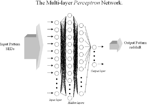
For each input pattern, the network produces an output pattern through the $propagation$ $rule$, compares the actual output with the desired one and computes an error. The learning algorithm adjusts the weights of the connections by an appropriate quantity to reduce the error (sliding down the slope). This process continues until the error produced by the network is low, according to a given criterion (see below).

2.1.1 The propagation rule

An input of a node ($net_{j}$) is the combination of the output of the previous nodes ($o_{i}$) and the weights of the corresponding links ($w_{ij}$), the combination is linear: $net_{j}=\sum_{i}w_{ij}o_{i}$. Each unit has a transform function (or activation function), which provides the output of the node as a function of the $net$. Nonlinear activation functions are needed to introduce nonlinearity into the network. We have used the logistic (or sigmoid) function: $out=1/[1+exp(-Knet)]$ and the $tanh$ function $out$=$tanh(Knet)$, for all units. $K$ is the gain parameter fixed before the learning. By increasing $K$ the activation function approximates a step. The propagation rule, from the input layer to the output layer, is a combination of activation functions.

No significant difference has been found in the training process between using the logistic and $tanh$ functions.

2.1.2 Back-propagation of the error

The weights, $\bf{w}$, are the free parameters of the network and the goal is to minimize the total error function with respect to $\bf{w}$ (maintaining a good generalization power, see below).

The error function in the weight space defines the multi-dimensional error surface and the objective is to find the global (or acceptable local) minima on this surface. The solution implemented in the present work is the $gradient\leavevmode\nobreak\ descent$, within which the weights are adjusted (from small initial random values) in order to follow the steepest downhill slope. The error surface is not known in advance, so it is necessary to explore it in a suitable way.

The error function typically used is the sum-of-squares error, which for a single input vector, $n$, is

$$e^{\{n\}}=\frac{1}{2}\sum_{i}\beta_{i}(y_{i}^{\{n\}}-T_{i}^{\{n\}})^{2}$$ (1)

where $y_{i}$ is the output of the NN and $T_{i}$ is the target output value for the $i^{th}$ output node and $n$ runs form 1 to the total number of examples in the training set. In the present work $i$=1, a single output node is used to estimate the redshift (other nodes could be used to estimate other quantities, such as the spectral type). The $\beta_{i}$ terms make it possible to assign different weights to different outputs, and thereby give priority to the correct determination of certain outputs. In the gradient descent process the weight vector is adjusted in the negative direction of the gradient vector,

$$\Delta{\bf w}=-\eta\frac{\partial e}{\partial{\bf w}}$$ (2)

and the new generic weight is

$$w_{new}=w_{old}+\Delta w$$

The amplitude of the step on the error surface is set by the $\eta$-learning parameter: large values of $\eta$ mean large steps. Typically $\eta$ belongs to the interval (0,1], in this application a small value has been used ($<0.005$) together with a high value of the gain in the activation functions ($K=5$). If $\eta$ is too small the training time becomes very long, while a large value can produce oscillations around a minimum or even lead to miss the optimal minimum in the error surface.

The learning algorithm used in the present work is the standard $back-propagation$. It refers to the method for computing the gradient of the case-wise error function with respect to the weights for a feed-forward network. $``Standard\leavevmode\nobreak\ backprop^{\prime\prime}$ is a definition of the $generalized$ $delta$ $rule$, the training algorithm that was popularized by Rumelhart, Hinton, and Williams in chapter 8 of Rumelhart and McClelland (1986), which remains one of the most widely used supervised training methods for neural nets.

This learning algorithm implies that the error function is continuous and derivable, so that it is possible to calculate the gradient. For this reason the activation functions (and their final combination through the propagation rule) must be continuous and derivable. From the computational point of view, the derivative of the activation functions adopted in the present work is easily related to the value of the function $out=F(net)$ itself (see Sec. 2.1.1: $F^{\prime}\propto out(1-out)$ in the case $F=sigmoid$ or $F^{\prime}\propto(1-out^{2})$ if $F=tanh$.)

Figure 2: A simplified representation of the error surface: the behavior of the error as a function of 2 weights. The momentum term improves the minimization during the training phase. Momentum allows a network to respond to the local gradient and also to take into account of the recent trends in the error surface. Acting like a low-pass filter, momentum allows the network to ignore small features in the error surface. Without momentum a network may get stuck in a shallow local minimum. With momentum a network can slide through such a minimum.

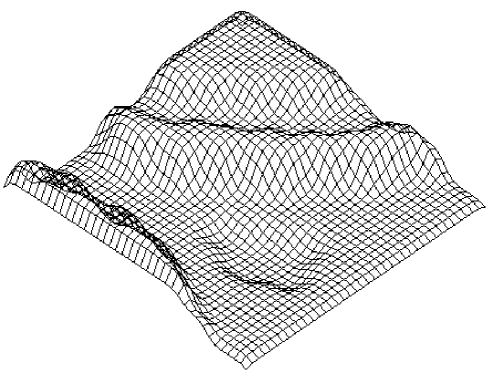
When the network weights approach a minimum solution, the gradient becomes small and the step size diminishes too, giving origin to a very slow convergence. Adding a momentum (a residual of the previous weight variation) to the equations of the weight update, the minimization improves (Bishop (1995)):

$$w_{new}=w_{old}+\Delta w+\alpha\Delta w_{old}$$ (3)

where $\alpha$ is the momentum factor (set to 0.9 in our applications). This can reduce the decay in learning updates and cause the learning to proceed through the weight space in a fairly constant direction. Besides a faster convergence to the minimum, this method makes it possible to escape from a local minimum if there is enough momentum to travel through it and over the following hill (see Fig. 2). The generalized delta rule including the $momentum$ is called the $``heavy\leavevmode\nobreak\ ball\leavevmode\nobreak\ method^{\prime\prime}$ in the numerical analysis literature (Bertsekas 1995, pg. 78- (79)).

The learning algorithm has been used in the so called on-line (or $incremental$) version, in which the weights of the connections are updated after each example is processed by the network. One $epoch$ corresponds to the processing of all examples one time. The other possibility is to compute the training in the so called $batch\leavevmode\nobreak\ learning$ (or epoch learning), in which the weights are updated only at the end of each epoch (not used in the present application).

3 The training technique

During the learning process, the output of a supervised neural net comes to approximate the target values given the inputs in the training set. This ability may be useful in itself, but more often the purpose of using a neural net is to generalize, i.e. to get some output from inputs that are $not$ in the training set ($generalization$). NNs, like other flexible nonlinear estimation methods such as kernel regression and smoothing splines, can suffer from either under fitting or over fitting. A network that is not sufficiently complex can fail to fully detect the signal in a complicated data set, leading to under fitting: an inflexible model will have a large $bias$. On the other hand a network that is too complex may fit the noise, not just the signal, leading to over-fitting: a model that is too flexible in relation to the particular data set will produce a large $variance$, (Sarle (1995)). The best generalization is obtained when the best compromise between these two conflicting quantities (bias and variance) is reached. There are several approaches to avoid under- and over-fitting, and obtain a good generalization. Part of them aim to regularize the complexity of the network during the training phase, such as the $Early\leavevmode\nobreak\ Stopping$ and $weight-decay$ methods (the size of the weights are tuned in order to produce a mapping function with small curvature, the large weights are penalized. Reducing the size of the weights reduces also the “effective” number of weights (Moody et al. (1992))).

A complementary technique belongs to the Bayesian framework, in which the bias-variance trade off is not so relevant, and networks with high complexity can be used without producing over-fitting (an example is to train a $committee$ of networks, Bishop (1995)).

3.1 Generalize error

3.1.1 Early stopping

The most commonly used method for estimating the generalization error in neural networks is to reserve part of the data as a $test\leavevmode\nobreak\ set$, which must not be used in $any$ way during the training. After the training, the network is applied to the test set, and the error on the test set provides an unbiased estimate of the generalization error, provided that the test set was chosen in a random way.

In order to avoid (possible) over-fitting during the training, another part of the data can be reserved as a $validation\leavevmode\nobreak\ set$ (independent both of the training and test sets, not used for updating the weights), and used during the training to monitor the generalization error. The best epoch corresponds to the lowest validation error, and the training is stopped when the validation error rate “starts to go up” ($early\leavevmode\nobreak\ stopping$ method). The disadvantage of this technique is that it reduces the amount of data available for both training and validation, which is particularly undesirable if the available data set is small. Moreover, neither the training nor the validation make use of the entire sample.

3.1.2 Committees of networks

As mentioned in the previous sections, an over-trained NN tends to produce a large variance in the predictions maintaining a relatively small bias. A method that reduces the variance (and keeps small the bias) is to use a committee of NNs (Bishop (1995)). Each member of the committee differs from the other members for the different training history. We have generated the members using a bootstrap process, varying:

1. the sequence of the input patterns (the incremental learning method used in the present work is dependent on the sequence presented).

2. the initial distribution of weights (the starting point on the error surface).

3. the architecture of the NN (number of nodes and layers).

The final prediction, adopted in the present work, is the mean and the median of the predictions obtained from the members of the committee (with 1-$\sigma$ error or 16 and 84 percentiles). Averaging over many solutions means reducing the variance. Since the complexity of the individual member is not a problem, the trainings have been performed without regularization and at the lowest training-error the weights have been frozen and used for the prediction.

This method has displayed a better and stable generalization power with respect to a single training (also using the validation set to regularize the learning). Moreover this method gives a robust estimate of the error bounds for the output of the network.

For these reasons the training described in the next sections has been carried out using a committee of networks.

4 The training-set

Since we are using a supervised neural network, we need a training-set. Each element (example) in the training-set is composed of a pair of vectors: the input pattern and the target. For our purposes the input pattern contains the Spectral Energy Distribution (SED) of the objects (but other configurations are possible: templates with a priori knowledge, SED plus the apparent luminosity in a reference band, the angular size, the morphology, etc.). The target in this application is the redshift.

The training has been tested on the available spectroscopic sample in the HDF–S (Cristiani et al. (2000), Rigopoulou et al. (2000), Vanzella et al. (2002), Glazebrook et al., http://www.aao.gov.au/hdfs/Redshifts/). The prediction of the redshifts in the HDF–S have been computed following different approaches:

1. training on the HDF–N spectroscopic sample using the colors as an input pattern.

2. training on the HDF–N spectroscopic sample using the colors and the apparent luminosity in the I band as an input pattern.

3. training on both HDF–N spectroscopic sample and a set of templates obtained from CWW (Coleman, Wu & Weedman) and/or from Rocca-Volmerange and Fioc (labelled RV00 hereafter).

4. Training on the CWW or RV00 SEDs alone (without spectroscopic redshifts) have also been tested.

The photometry of the HDF–N has been obtained from the available catalog provided by Fernández-Soto, Lanzetta & Yahil (1999) whereas the photometric catalog of the HDF–S is provided by Vanzella et al. (2001) and Fontana et al. (2003).

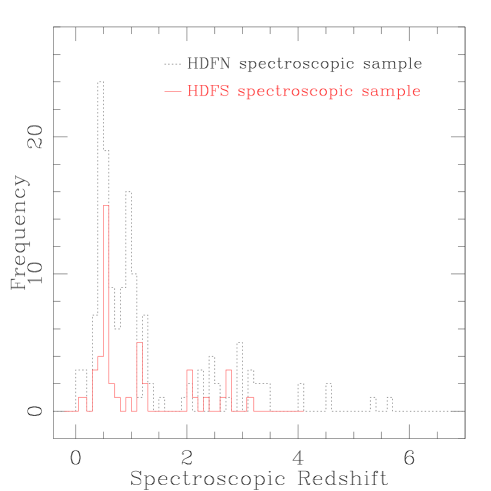
The sample in the HDF–N contains 150 spectroscopic redshifts (Cohen et al. (2000), Dawson et al. (2001), Fernández-Soto et al. (2001)), while the sample in the HDF–S contains 44 spectroscopic redshifts (in Fig. 3 the redshift distributions of both fields are shown).

Figure 3: Spectroscopic redshift distributions of the two fields HDF–N (dashed line) and HDF–S (solid line).

In order to test the prediction we have used the variance as a statistical estimator:

$$\sigma_{z}^{2}=\frac{1}{N}\sum_{i}(zNN_{i}-zspec_{i})^{2}\ \ .$$

where $zNN$ is the neural prediction, $N$ is the number of galaxies, and $i$=1..$N$. In the literature another statistical estimator is sometimes used, the mean absolute deviation normalized by the $(1+z)$ factor (e.g. Labbé et al. (2003)):

$$\delta_{z}=\frac{1}{N}\sum_{i}\frac{|zNN_{i}-zspec_{i}|}{1+zspec_{i}}\ \ .$$

The quantity $\delta_{z}$ has the advantage to be roughly uniform, while the variance tends to increase with increasing redshift.

4.1 The input pattern

The magnitudes of the observed objects in a given photometric system are the input of the network. In the present work the filters are $F300$, $F450$, $F606$, $F814$ (WFPC2, HST) and $Js$, $H$, $Ks$ for the near infrared (ISAAC, VLT). If the flux in a given band has a signal to noise ratio less than 2.0 it is considered an upper limit in that band, and the value of the flux is set to 1$\sigma$ error.

It is convenient to avoid too large input values that could cause a saturation in the output of the activation functions (sigmoid or $tanh$), but it is not necessary to rescale the inputs rigorously in the interval [-1,1]. A non linear rescaling of the input values is also useful to make more uniform the function that the network is trying to approximate.

In the present application the input values have been rescaled: $p_{i}=-0.5+[f_{i}/f_{F814}]^{0.4}$, where $i$ runs over the following bands: $F300$, $F450$, $F606$, $Js$, $H$, $Ks$ and $f_{F814}$ is the flux in the reference $F814$ band. When the apparent AB magnitude in the $F814$ band, $m_{814}$, is used as an input (e.g. Sec. 5.1.2 and 5.2.2), it has been normalized as follow:

$$p_{F814}=\left[\frac{1}{(m_{max}-m_{min})}\right]([m_{814}-m_{min}]-[m_{max}-m_{814}])$$

where $m_{max}$ is 28 and $m_{min}$ is 18.

5 Redshift prediction on the HDF–S

Table 1: Training of different architectures on the HDF–N spectroscopic sample (150 objects) and evaluation on the HDF–S spectroscopic sample. The number of epochs is 5000, the bootstrap has been computed on 100 extractions (100 members of the committee).

$Colors$ as				$Colors$ $\&$ $Magnitudes$
input pattern				as input pattern
[Net]_Weights	$<\sigma_{z}^{train}>$	$\sigma_{z}^{test}$	$\delta_{z}^{test}$	[Net]_Weights	$<\sigma_{z}^{train}>$	$\sigma_{z}^{test}$	$\delta_{z}^{test}$
		median/mean	median/mean			median/mean	median/mean
[6:10:10:1]_181	0.100	0.190/0.193	0.074/0.078	[7:10:10:1]_201	0.090	0.163/0.171	0.065/0.065
[6:10:9:1]_179	0.103	0.191/0.191	0.074/0.075	[7:10:9:1]_189	0.087	0.174/0.173	0.067/0.065
[6:10:8:1]_167	0.103	0.193/0.203	0.074/0.079	[7:10:8:1]_177	0.083	0.166/0.172	0.066/0.067
[6:10:7:1]_155	0.107	0.192/0.195	0.074/0.075	[7:10:7:1]_165	0.090	0.167/0.175	0.066/0.065
[6:10:6:1]_143	0.107	0.191/0.203	0.076/0.079	[7:10:6:1]_153	0.090	0.162/0.174	0.063/0.066
[6:10:5:1]_131	0.110	0.172/0.184	0.070/0.073	[7:10:5:1]_141	0.093	0.162/0.184	0.064/0.069
[6:9:5:1]_119	0.110	0.183/0.200	0.074/0.078	[7:9:5:1]_128	0.097	0.155/0.171	0.058/0.061
[6:8:5:1]_107	0.120	0.187/0.209	0.075/0.079	[7:8:5:1]_115	0.103	0.158/0.177	0.062/0.065
[6:7:5:1]_95	0.120	0.190/0.214	0.075/0.080	[7:7:5:1]_102	0.103	0.147/0.161	0.056/0.058
[6:6:5:1]_83	0.133	0.211/0.230	0.075/0.077	[7:6:5:1]_89	0.113	0.149/0.159	0.059/0.061
[6:5:5:1]_71	0.153	0.216/0.227	0.076/0.078	[7:5:5:1]_76	0.130	0.140/0.155	0.057/0.060
[6:5:4:1]_64	0.153	0.233/0.247	0.080/0.083	[7:5:4:1]_69	0.130	0.144/0.156	0.059/0.062
[6:5:3:1]_57	0.167	0.263/0.290	0.086/0.093	[7:5:3:1]_62	0.137	0.159/0.170	0.062/0.064
[6:5:2:1]_50	0.213	0.275/0.269	0.088/0.087	[7:5:2:1]_55	0.150	0.154/0.156	0.060.0.061
[6:5:1:1]_43	0.303	0.291/0.290	0.126/0.125	[7:5:1:1]_48	0.240	0.194/0.195	0.074/0.074
[6:20:1]_161	0.300	0.283/0.281	0.117/0.118	[7:20:1]_181	0.237	0.226/0.225	0.086/0.084
[6:15:1]_122	0.293	0.277/0.275	0.116/0.118	[7:15:1]_136	0.230	0.228/0.229	0.087/0.085
[6:10:1]_81	0.273	0.259/0.258	0.105/0.106	[7:10:1]_91	0.223	0.207/0.219	0.083/0.084
[6:5:1]_41	0.340	0.287/0.289	0.117/0.120	[7:5:1]_46	0.273	0.261/0.259	0.097/0.097
${\dagger}$ [—] _83..215	0.105	0.190/0.206	0.071/0.075	[—]_93..225	0.086	0.175/0.186	0.065/0.065

${\dagger}$ Training and combination of different architectures (n:10:1..12:1). In the second hidden layer the number of units ranges from 1 to 12.

5.1 Training on the HDF–N

5.1.1 Colors as input pattern

Figure 4: Comparison between spectroscopic redshift in the HDF–S and the neural redshift using the colors as an input pattern. The training has been done on the HDF–N spectroscopic sample, the estimation of the redshift for each object is the median of 100 predictions and the error bars represent 1-$\sigma$ interval. Open circles represent objects with unreliable photometry and triangles are objects with uncertain spectroscopic redshift.

Figure 5: The effects of adding information. Upper panel: comparison between spectroscopic redshift and the neural redshift for the spectroscopic sample in the HDF–S. The training has been carried out on the HDF–N spectroscopic sample (150 objects, as shown in the lower panel of the Fig. 4). The partial error ($\sigma_{part}$) has been considered, i.e. the dispersion calculated without the three objects marked with the open square symbols, see text). Lower panel: comparison between spectroscopic redshift and the neural redshift for the spectroscopic sample in the HDF–S, the open squares symbols show the three objects that have been used during the training (in addition to the 150 objects in the HDF–N), this new information improves the partial error (i.e. the $\sigma_{part}$ calculated without these three objects), in particular at redshift around 1.2.

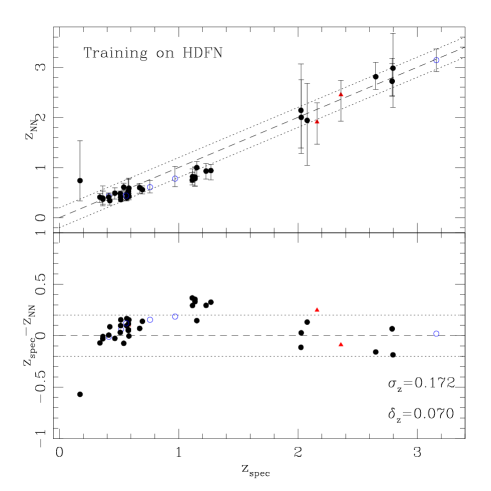
The input pattern contains the colors of the galaxies ($\frac{f_{F300}}{f_{F814}}$, $\frac{f_{F450}}{f_{F814}}$, $\frac{f_{F606}}{f_{F814}}$, $\frac{f_{J}}{f_{F814}}$, $\frac{f_{H}}{f_{F814}}$, $\frac{f_{K}}{f_{F814}}$), normalized as described in Section 4.1.

The training has been carried out setting the maximum number of epochs to 5000. The distribution of weights corresponding to the minimum training error has been stored. We have verified that 5000 epochs are sufficient in this case to reach the convergence of the system. Trainings done on 10000 and 15000 epochs give similar results.

The dispersion $\sigma_{z}^{test}$ obtained for the spectroscopic sample in the HDF–S is shown in Table LABEL:tab:architecture (left side). Different architectures have been used with one and two hidden layers and different numbers of nodes.

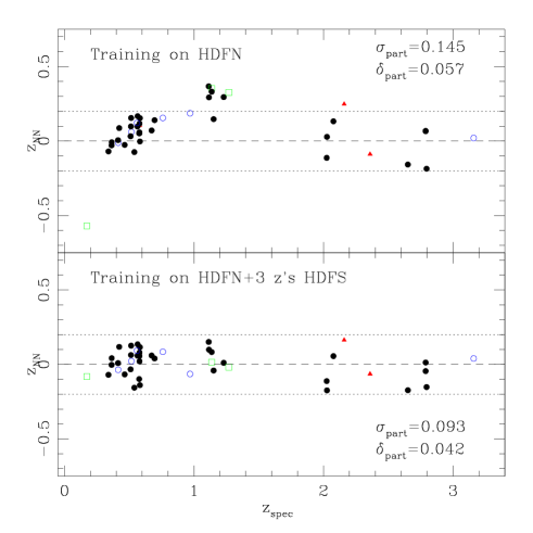
The comparison between $zspec$ and $zNN$ for the architecture 6:10:5:1 (six input nodes, two hidden layers with ten and five units and one output nodes) is shown in Fig. 4. The resulting error is $\sigma_{z}^{test}=0.172$. The systematic errors are common to all the explored architectures. In particular there is a clear discrepancy for the object at $z=0.173$ (ID=667 in the Tables of Vanzella et al. (2001)), due to the insufficient information available in that redshift regime. A systematic underestimation for the group of objects at redshift around 1.2 is also evident. Combining different architectures with different numbers of units in the second hidden layer (from 1 to 12), the result does not change, the dispersion in the test set is compatible with the dispersion obtained using a fixed architecture.

For networks with a low complexity the error ($\sigma_{z}^{test}$) starts increasing together with the $<\sigma_{train}>$ (the $<\sigma_{train}>$ is the mean of the training errors ($\sigma_{train}$) obtained in the bootstrap). The same happens with networks with one hidden layer (see Table LABEL:tab:architecture).

These results show that, although one hundred extractions (100 members) are enough to diminish the random errors, new information in the training set is needed in order to reduce the systematic errors.

This is clearly shown in Fig. 5 where we have added to the training set three objects belonging to the HDF–S spectroscopic sample: ID=667 with the discrepant redshift mentioned above and two objects randomly chosen from the group around redshift 1.2. In the upper panel of Fig. 5 the square symbols represent these three objects used in the training together with the 150 in the north, the dispersion in the HDF–S is calculated on the rest of the sample (41 objects, $\sigma_{part}$). The training on the 150 objects gives as prediction $\sigma_{part}$=0.145. By computing the training in the same conditions but with 153 objects rather than 150, the prediction around redshift 1.2 clearly improves, and a $\sigma_{part}$=0.093 is obtained. The predictions for the rest of the objects do not change significantly. The improvement for the square symbols is obvious (it is due to the learning algorithm). The network shows a remarkable ability to learn the new signal present in the training set.

In the next section the colors together with the apparent luminosity in the $F814$ band will be used as input pattern.

5.1.2 Colors and apparent luminosity as an input pattern

Figure 6: Comparison between spectroscopic redshift and the neural redshift for the spectroscopic sample in the HDF–S. The training has been carried out on the HDF–N spectroscopic sample, the estimation of the redshift for each object is the median of 100 predictions. The input pattern is composed of colors and the apparent luminosity in the $F814$ band. The symbols are the same as in Fig. 4.

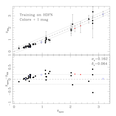
The input pattern contains the colors and the apparent luminosity in the $F814$ band. Also in this case we have performed one hundred training on the 150 galaxies in the HDF–N. The dispersion $\sigma_{z}^{test}$ obtained for the spectroscopic sample in the HDF–S is shown in Table LABEL:tab:architecture (right side, “colors $\&$ mag.”). In general, the predictions are better than the results obtained with only colors as an input pattern. In this application the magnitude information improves the prediction at low redshift (in particular for the object ID=667). On the other hand the scatter at high redshift seems to increase, if compared with the case with only colors as an input (see Fig. 6). There is still a bias (although reduced) at redshifts around 1.2.

The training on different architectures, 6:10:1:1, 6:10:2:1, … and 6:10:12:1 (6:10:1..12:1 hereafter) produces a dispersion similar to that obtained by fixing the architecture. Also in this case the networks with a low complexity produce a large error both in the $<\sigma_{train}>$ and in the $\sigma_{z}^{test}$. The same happens with networks with one hidden layer (see Table LABEL:tab:architecture).

These tests show that the information introduced by the apparent luminosity produces a slight improvement: the error is always less than the error obtained using only colors (but the sample is still too small to generalize this result).

The problem concerning the completeness of the training set is common in the empirical technique for the estimation of the redshift. There is a well known gap without spectroscopic redshifts in the interval (1.3,2) due to the absence of observational spectroscopic features. Moreover, spectroscopic surveys are flux limited and the spectroscopic redshifts tend to be available only for brighter objects. To solve this problem and fill the above mentioned gap it is useful to introduce in the training set examples derived from observed or synthetic template SEDs.

Table 2: Training of different architectures on the HDF–N spectroscopic sample and a set of templates derived from CWWK. The evaluation is on the HDF–S spectroscopic sample. The bootstrap has been computed on 100 extractions (100 members of the committee). In the “training data” column, “+150” means that the 150 spectroscopic redshifts in the HDF–N have been used in addition to the CWWK SEDs.

[Net]_Weights	Epochs	Training	$dz$	E(B-V)	$<\sigma_{train}>$	$\sigma_{z}^{test}$	$\delta_{z}^{test}$
		Data				median/mean	median/mean
[6:30:30:1]_1171	1000	3206+150	0.01	0	0.059	0.142/0.143	0.054/0.056
[6:25:25:1]_851	1000	3206+150	0.01	0	0.078	0.132/0.133	0.057/0.056
[6:20:20:1]_581	1000	3206+150	0.01	0	0.062	0.131/0.128	0.056/0.054
[6:15:15:1]_361	1000	3206+150	0.01	0	0.065	0.135/0.128	0.058/0.055
[6:15:10:1]_276	1000	3206+150	0.01	0	0.064	0.131/0.127	0.058/0.055
[6:10:15:1]_251	1000	3206+150	0.01	0	0.078	0.128/0.127	0.060/0.059
[6:10:10:1]_191	1000	3206+150	0.01	0	0.076	0.138/0.133	0.064/0.060
[6:10:5:1]_131	1000	3206+150	0.01	0	0.076	0.138/0.132	0.064/0.062
[6:7:6:1]_104	1000	3206+150	0.01	0	0.106	0.159/0.157	0.076/0.075
[6:5:5:1]_71	1000	3206+150	0.01	0	0.173	0.198/0.186	0.084/0.080
[6:20:20:1]_581	500	12824+150	0.01	0.0,0.05,0.1,0.2	0.060	0.132/0.135	0.056/0.055
[6:15:10:1]_276	5000	646+150	0.05	0	0.068	0.125/0.127	0.057/0.057
[6:15:10:1]_276	5000	326+150	0.1	0	0.093	0.127/0.128	0.059/0.060
*[6:10:1..12:1]_83..251	10000	326+150	0.1	0	0.086	0.134/0.133	0.062/0.062
* Training on different architectures, in the second hidden layer the number of units ranges from 1 to 12 (6:10:1..12:1).

Figure 7: Comparison between spectroscopic redshift in the HDF–S and the neural redshift obtained with a committee of networks and using as input pattern the colors. The estimation of the redshift for each object is the mean of 100 predictions and the error bars represent 1-$\sigma$ interval. The training set is composed by CWWK SEDs mixed with the spectroscopic sample in the HDF–N. The symbols are the same as in Fig. 4.

5.2 Combination of training sets

5.2.1 Training on HDF–N mixed with CWW SEDs

Increasing the information in the training data is an obvious method to improve the generalization.

As a first approach to produce a complete range of galaxy SEDs we have adopted the templates of Coleman, Wu & Weedman (1980) for a typical elliptical, Sbc, Scd and Irregular galaxy plus two spectra of star-forming galaxies (SB1 and SB2 from the atlas of Kinney et al. (1996)). This choice is similar to the approach of Fernández-Soto, Lanzetta & Yahil (1999) and Arnouts et al. 1999a and in the following will be referred to as “CWWK”.

Galaxies have been simulated in the redshift range 0$<$z$<$6. 3206 SEDs have been drawn from the CWWK templates with a step in redshift equal to 0.01 ($dz=0.01$). Extinction effects have been introduced ($E(B-V)=0.05,0.1,0.2$) adopting a Calzetti extinction law (Calzetti (1997)). 12824 SEDs have been produced in this way. The CWWK templates do not take into account the evolution of galaxy SEDs with cosmic time.

A committee of 100 networks has been adopted and the median and mean values have been used to estimate the redshift.

In Table 2 the prediction for the HDF–S spectroscopic sample is shown. A series of tests has been carried out both neglecting the effects of intrinsic extinction and introducing an extinction effect. No significant difference in the predictions has been measured. The number of training data and the $<\sigma_{train}>$ are also shown.

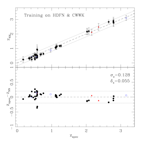
The predictions for the HDF–S are clearly improved taking into account the information derived from the CWWK templates and remain stable almost independently of the architecture ($\sigma_{z}^{test}\simeq 0.13$). Low complexity networks (6:7:6:1 and 6:5:5:1) produce large errors: these are clear cases of under-fitting in the training data. In Fig. 7 the comparison between the spectroscopic redshifts and the neural predictions is shown for the network 6:15:15:1 and bootstrap process. The prediction improves at redshift around 1 and for the object ID=667 at $z=0.173$. At high redshift ($z>2$) the uncertainty of the individual redshift estimates is significantly reduced (compare, for example, the error bars at $z>2$ in Fig. 4 and in Fig. 7).

Reducing the step in redshift ($dz$=0.01, 0.05, 0.1) and hence the number of training data, leaves the prediction stable. The trainings computed on a reduced sample, 326+150 examples (326 CWWK SEDs and 150 spectroscopic redshifts in the HDF–N) with $dz=0.1$ and 646+150 examples with $dz=0.05$ without extinction, give the same result obtained with $dz=0.01$. This means that the committee of networks is able to achieve the same fit in the color space also with a reduced grid.

Figure 8: Comparison between spectroscopic redshift in the HDF–S and the neural redshift obtained with a committee of networks and using as input pattern the colors. The estimation of the redshift for each object is the mean of 100 predictions and the error bars represent 1-$\sigma$ interval. The training set is composed of RV00 models (bootstrap on 1000 RV00 SEDs and 150 spectroscopic redshifts in the HDF–N, see Table LABEL:tab:RV00). The symbols are the same as in Fig. 4.

Figure 9: Predictions of a (6:20:20:1) NN for 44 galaxies in the HDF–S as a function of the epoch (an epoch correspond to the processing of all the examples one time, as defined in Sect. 2.1.2). The training has been carried out on the spectroscopic sample in the HDF–N and on RV00 templates, using as an input pattern the colors and the I mag. The ordinate shows the difference between the prediction of the NN, $z_{NN}$, at a given epoch and the actual spectroscopic redshift $z_{spec}$. The numbers in the upper left part of the panels correspond to the galaxy identifiers in the catalog by Vanzella et al. (2001).

5.2.2 Training on the HDF–N mixed with Pegase models

We have also trained the neural system on the HDF–N spectroscopic sample and a set of models derived from the most recent version of the code by M. Fioc and Rocca-Volmerange (Fioc & Rocca-Volmerange (1997)), named Pegase 2.0 (RV00).

In the Rocca–Volmerange code the star formation history is parameterized by two $e-folding$ star formation time-scales, one ($\tau_{g}$) describing the time–scale for the gas infall on the galaxy and the other ($\tau_{*}$) the efficiency of gas to star conversion. By tuning the two time–scales it is possible to reproduce a wide range of spectral templates, from early types (by using small values of $\tau_{g}$ and $\tau_{*}$) to late types. For the earliest spectral type, a stellar wind is also assumed to block any star–formation activity at an age $t_{wind}$. The major advantage of the Rocca–Volmerange is that it allows to follow explicitly the metallicity evolution, including also a self–consistent treatment of dust extinction and nebular emission. Dust content is followed over the galaxy history as a function of the on–going star–formation rate, and an appropriate average over possible orientations is computed. Although more model–dependent, this approach has the advantage of producing the evolutionary tracks of several galaxy types with a self–consistent treatment of the non-stellar components (dust and nebular emission). An application of the PEGASE 2.0 code to photometric redshifts has been recently presented by Le Borgne & Rocca-Volmerange (2002).

We have followed the training technique described in Sec. 3.1.2. Adopting the scenarios described in Le Borgne & Rocca-Volmerange (2002) we have obtained three samples from the RV00 package: 112824, 28544 and 14400 models with step in redshift $dz=0.025$, $dz=0.1$ and $dz=0.2$, respectively (0$<z<$6). An other training sample has been obtained from the 112824 sample dimming the fluxes by a factor of 10 and 100 and considering as the training set the templates with apparent luminosity in the $F814$ band less than 27, in this way 201757 objects have been carried out.

Table 3: Training of different architectures on the HDF–N spectroscopic sample and a set of templates derived from Rocca Volmerange (redshift in the interval $z=0-6$). The evaluation is on the HDF–S spectroscopic sample. The bootstrap has been computed on 100 extractions (100 members of the committee). In the training data column, “+150” means that the 150 spectroscopic redshifts in the HDF–N have been used in addition to the RV00 models.

[Net]_Weights	Epochs	Training	$dz$	$<\sigma_{train}>$	$\sigma_{z}^{test}$	$\delta_{z}^{test}$
		Data			median/mean	median/mean
[6:20:20:1]_581	2000	1000+150	0.025	0.168	0.118/0.120	0.047/0.050
[6:20:20:1]_581	3000	300+150	0.1	0.171	0.123/0.119	0.054/0.053
[6:20:20:1]_581	5000	150+150	0.2	0.142	0.123/0.116	0.053/0.051
[6:30:30:1]_1171	2000	1000+150	0.025	0.167	0.125/0.119	0.048/0.050
[6:20:20:1]_581	2000	1000+150	0.025	0.168	0.118/0.120	0.047/0.050
[6:10:10:1]_191	2000	1000+150	0.025	0.176	0.111/0.123	0.047/0.052
[6:5:5:1]_71	2000	1000+150	0.025	0.223	0.159/0.164	0.064/0.068

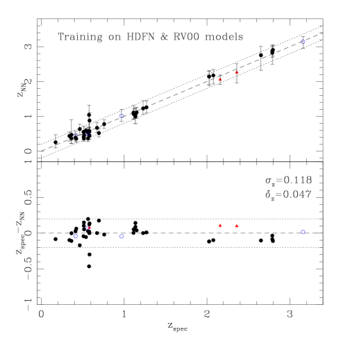
In the training on mixed samples the RV00 templates produce slightly better results than the CWWK SEDs. A bootstrap process of 100 extractions has been carried out: at each extraction a random sequence of the input patterns and a random initialization of the weights have been adopted. At each extraction the training has been computed on a set of data composed by 150 spectroscopic redshifts in the HDF–N and a subset of models extracted randomly from the RV00 samples. The performance in the south sample is $\sigma_{z}^{test}\simeq 0.12$ (see Table LABEL:tab:RV00).

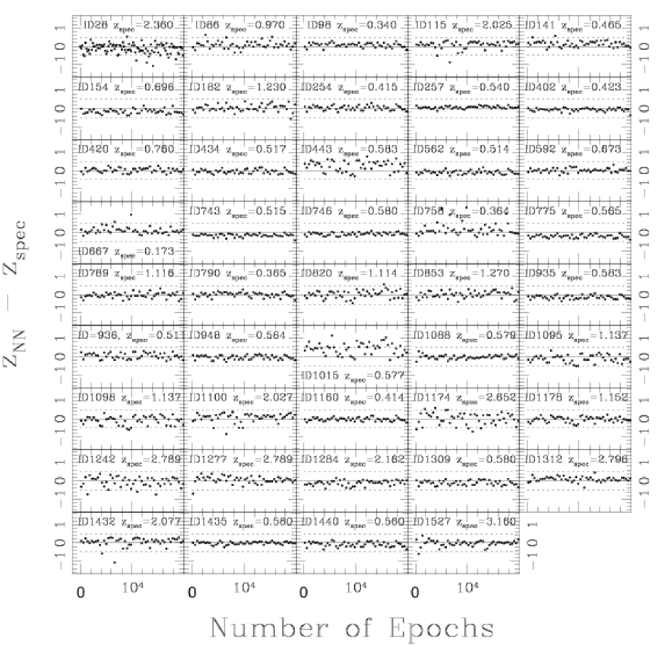
Fig. 9 shows that no significant trend is present over the epochs varying the initial distribution of weights and the sequence of the training data (in the abscissa the epochs and in the ordinate the difference $zNN-zspec$). The prediction of the network becomes stable after the first epochs (greater than 500) until the maximum epoch (20000). The spread in the plots gives an indication of the resulting uncertainty (also the spread is stable over the epochs).

Adopting a training set composed of RV00, CWWK and the spectroscopic sample in the HDF–N produces a $\sigma_{z}^{test}\simeq 0.12$, of the same order of the dispersions obtained with RV00+HDF–N and CWWK+HDF–N as training sets.

5.2.3 Training on CWWK or RV00 templates

Table 4: Training with various NN architectures on templates derived from CWWK and RV00. The bootstrap has been computed on 100 extractions (100 members of the committee).

[Net]_Weights	Epochs	Training	$dz$	E(B-V)	$<\sigma_{train}>$	$\sigma_{z}^{test}$	$\delta_{z}^{test}$	sample
		Data				median/mean	median/mean
[6:20:20:1]_581	1000	3206${}_{\ CWWK}$	0.01	0	0.036	0.180/0.186	0.068/0.067	HDF–S
[6:20:20:1]_581	500	12824${}_{\ CWWK}$	0.01	0,0.05,0.1,0.2	0.044	0.196/0.200	0.067/0.068	HDF–S
[7:20:20:1]_601	10	201757${}_{\ RV00}$	0.025	-	0.157	0.153/0.158	0.068/0.070	HDF–S
[7:20:20:1]_601	10	201757${}_{\ RV00}$	0.025	-	0.157	0.259/0.257	0.061/0.062	HDF–N
[7:20:20:1]_601	10	201757${}_{\ RV00}$	0.025	-	0.157	0.231/0.233	0.064/0.064	HDF–N/S

Figure 10: Comparison between spectroscopic redshift in the HDF–S and the neural redshift obtained with a committee of networks and using as input pattern the colors. The estimation of the redshift for each object is the mean of 100 predictions and the error bars represent 1-$\sigma$ interval. The training set is composed of CWWK SEDs (3206 SEDs, see Table 2). The symbols are the same as in Fig. 4.

Figure 11: Comparison between spectroscopic redshift in the HDF–S and the neural redshift obtained with a committee of networks and using as input pattern the colors. The estimation of the redshift for each object is the mean of 100 predictions and the error bars represent 1-$\sigma$ interval. The training set is composed of RV00 models (112824 SEDs, see Table LABEL:tab:RV00). The symbols are the same as in Fig. 4.

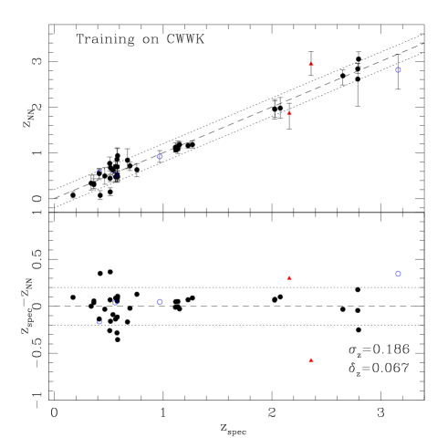
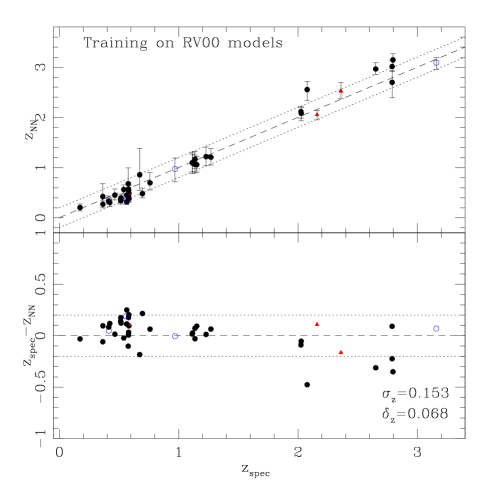
Table LABEL:tab:onlyTemplates summarizes the results of various trainings carried out only on templates, without the spectroscopic redshifts.

Training on the colors derived from the CWWK templates produces a dispersion in the HDF–S sample $\sigma_{z}^{test}=0.186/0.180$ (mean/median) (see Fig. 10). A redshift step $dz=0.01$ and an extinction $E(B-V)=0.0$ were adopted (3206 SEDs in the training set). A bootstrap on 100 extractions with maximum number of epochs set to 1000 was carried out. Again, introducing the effects of extinction does not improve this result.

Training on the colors and the apparent luminosity in the $F814$ band (7 inputs) derived from the RV00 models produces a dispersion in the HDF–S sample $\sigma_{z}^{test}=0.158/0.153$ (mean, median), better than the estimates obtained with the CWWK SEDs.

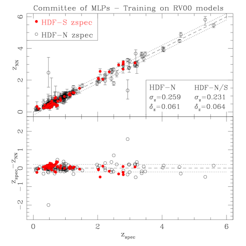
Fig. 12 compares the prediction of a NN trained on the RV00 templates with the spectroscopic redshifts in the HDF–N and HDF–S. The dispersion turns out to be $\sigma_{z}^{test}=0.231$ for the full HDF–N plus HDF–S sample and $0.259$ for the HDF–N only.

Figure 12: Comparison between spectroscopic redshifts (HDF–N and HDF–S) and the neural redshifts obtained with a committee of networks, using as an input pattern the colors and the apparent luminosity in the $F814$ band derived from RV00 models. The estimation of the redshift for each object is the median of 100 predictions and the error bars represent the 1-$\sigma$ interval.

Table 5: Summary of the different tests performed on the HDF–S spectroscopic sample ($z<3.5$, 44 objects) described in Section 5. The dispersion $\sigma_{z}$ is calculated in a low redshift regime $z<2$ (34 objects) and high redshift regime $z>2$ (10 objects).

Training set	$\sigma_{z}\leavevmode\nobreak\ (z<3.5)$	$\sigma_{z}\leavevmode\nobreak\ (z<2)$	$\sigma_{z}\leavevmode\nobreak\ (z>2)$
	44 objs.	34 objs.	10 objs.
HDF–N	0.172	0.186	0.114
HDF–N mag.	0.162	0.139	0.222
CWWK & HDF–N	0.128	0.131	0.114
RV00 & HDF–N	0.118	0.128	0.094
CWWK	0.186	0.146	0.282
RV00	0.153	0.115	0.237

In Table LABEL:tab:summary the tests on the HDF–S spectroscopic sample are summarized. The dispersion is calculated for 44 objects at $z<3.5$ and separately in the low-redshift ($z<2$) and high-redshift ($z>2$) regimes. In general the performance improves when the information in the training set increase.

6 Application to the SDSS DR1

Figure 13: Redshift distribution of the spectroscopic sample obtained from the SDSS DR1 (113000 galaxies, solid line). The dashed line represents the distribution of the neural redshift prediction of the test sample (88108 galaxies) normalized to the total sample obtained with a 19:12:10:1 architecture (see text).

The Sloan Digital Sky Survey (SDSS; York et al. (2000)) consortium has publicly released 134015 spectroscopic redshifts (Abazajian et al. (2003)). The photometry in the $ugriz$ bands and various image morphological parameters are also available.

Recently, Tagliaferri et al. (2002) and Firth et al. (2002) have used neural networks to produce photometric redshifts based on the SDSS Early Data Release (SDSS EDR, Stoughton et al. (2002)), while Ball et al. (2003) have applied neural networks to the DR1 sample.

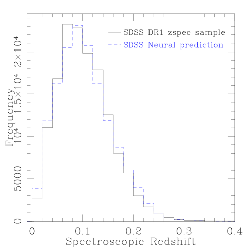
We have selected the data with the following criteria (see also Firth et al. (2002)): (1) the spectroscopic redshift confidence must be greater than 0.95 and there must be no warning flags, (2) $r<17.5$. Moreover we have adopted the photometric criteria proposed in Yasuda at al. (2001) for the star-galaxy separation. An object is classified as a star in any band if the model magnitude and the PSF magnitude differ by no more than 0.145. The resulting catalog is almost entirely limited to $z<0.4$. The redshift distribution of the DR1 sample is shown in Fig. 13.

Two different approaches have been explored in the NN estimation of the DR1 photometric redshifts:

1. A 7:12:10:1 network with 3000 epochs and 10 different trainings, carried out changing the initial random distributions of weights and the sequence of the training examples. The “best” distribution of weights corresponds to the lowest error in the training sample (in almost all cases coincident with the last epoch). The 7 input nodes are: the colors, the $r$-band magnitude, the Petrosian 50 and 90 per cent $r$-band flux radii ($u-g$, $g-r$, $r-i$, $i-z$, $r$, $PetR50$, $PetR90$).

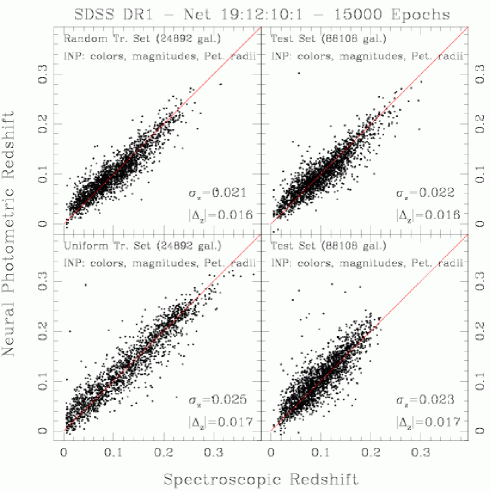
2. A 19:12:10:1 network with 15000 epochs and a single training carried out. The additional inputs are in this case the u-, g-, i-, z-band magnitudes and the Petrosian 50 and 90 per cent flux radii in these bands.

The results in terms of dispersions ($\sigma_{z}$ and $|\Delta_{z}|$) and mean offsets $<\Delta_{z}>$ are summarized in Table LABEL:tab:TAB_SLOAN.DR1.

Table 6: SDSS - DR1: Training on 24892 galaxies (uniform and random sample). Test on 88108 galaxies. The mean values are derived from 10 trainings by varying the initial random distribution of weights and the sequence of the training examples. In the first 2 rows 7 inputs nodes have been used (u-g, g-r, r-i, i-z, r, PetR50, PetR90). Rows 3 and 4 correspond to a single training and 19 inputs have been used (u-g, g-r, r-i, i-z, u, g, r, i, z, PetU50, PetU90, PetG50, PetG90, PetR50, PetR90, PetI50, PetI90, PetZ50, PetZ90).

Net	$\bf{W}$	Epochs	Training	$<\sigma_{z}>$	$<|\Delta_{z}|>$	$<\Delta_{z}>$	$<\sigma_{z}>$	$<|\Delta_{z}|>$	$<\Delta_{z}>$
			Data	(Train)	(Train)	(Train)	(Test)	(Test)	(Test)
7:12:10:1	273	3000	24892unif	0.026$\pm$0.0002	0.018$\pm$0.0002	0.000	0.024$\pm$0.0007	0.017$\pm$0.0005	0.004
7:12:10:1	273	3000	24892rand	0.023$\pm$0.0005	0.017$\pm$0.0004	0.000	0.023$\pm$0.0004	0.017$\pm$0.0004	0.002
Net	$\bf{W}$	Epochs	Training	$\sigma_{z}$	$|\Delta_{z}|$	$<\Delta_{z}>$	$\sigma_{z}$	$|\Delta_{z}|$	$<\Delta_{z}>$
19:12:10:1	381	15000	24892unif	0.025	0.017	0.002	0.023	0.017	0.001
19:12:10:1	381	15000	24892rand	0.021	0.016	-0.001	0.022	0.016	-0.002

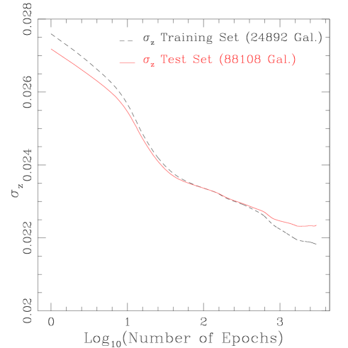
Increasing the number of input nodes and the number of epochs improves only slightly the result. In particular, Fig. 14 shows the behavior of the training error for the 19:12:10:1 network as a function of the “current” epoch, shown until the maximum epoch 3000. It is worth noting that, because of the incremental learning method used in the present work (see Sect. 2.1.2), each epoch corresponds to a number of variations of weights equal to the number of training examples in the training set. This explains why the predictions of the network are good also at the very beginning (epoch 1) of the training phase.

Figure 14: Behavior of the prediction as a function of the epochs for the SDSS DR1 sample. The non-uniform training sample has been used with the 19:12:10:1 architecture. 3000 epochs have been computed, the training and test errors are shown as a function of the epoch.

The highly inhomogeneous distribution of the redshifts (see Fig. 13) is expected to produce a bias in the estimates, as discussed in Tagliaferri et al. (2002), since any network will tend to perform better in the range where the density of the training points is higher. To investigate this effect two types of training have been carried out: on a uniform training set and a randomly extracted training set. The random and the uniform training sets are both made of 24892 galaxies. In the cases of randomly extracted training sets (Fig. 15 upper panels), a trend in the training and test phase is evident. It appears as a distortion around z$\simeq$0.1, corresponding to the higher density of training points (see Fig. 13). The behavior of the diagram using a uniform training set is more regular (Fig. 15 lower panels).

Figure 15: Redshift prediction in the SDSS DR1 (113000 galaxies) spectroscopic sample using a 19:12:10:1 architecture, 3000 epochs and 19 inputs (u-g, g-r, r-i, i-z, u, g, r, i, z, PetU50, PetU90, PetG50, PetG90, PetR50, PetR90, PetI50, PetI90, PetZ50, PetZ90) as input pattern. In the lower panel (training set on the left, test set on the right) the training set has been built adopting a grid with a fixed step $dz$=0.000012 and extracting one galaxy for each interval of the grid (24892 galaxies in total). In the upper panel (training set on the left, test set on the right) the training set has been built extracting randomly a sample of the same size (24892 galaxies) of the uniform sample. In left panels only one point every 16 is plotted, while in the right panels only a point every 50 is plotted.

Due to the large amount of data available, the trainings with and without the validation set have produced indistinguishable results. Also the dispersion obtained with a committee of networks and with a single member is comparable, therefore no regularization has been applied and a single training has been adopted in all cases.

Increasing the number of connections in the architecture of the network does not cause the results to change significantly. It is interesting to note that even with a simple network 7:2:5:1 (34 weights and 7 input neurons), the dispersion obtained is comparable to the 381 weights net (19:12:10:1). The 7:2:5:1 gives $\sigma_{z}\simeq 0.027$ ($|\Delta_{z}|\simeq 0.021$) in the 88108 test galaxies sample.

Various photometric redshift techniques (template-fitting, Bayesian method, polynomial fitting, nearest-neighbor etc.) have been applied to a similar spectroscopic sample extracted from the SDSS EDR (see Csabai et al. (2002)). They produce in general significantly worse results in terms of redshift dispersion, except for the “Kd-tree”, which shows a $\sigma_{z}=0.025$.

Figure 16: Comparison between spectroscopic redshift in the HDF–S and the neural redshift obtained with a committee of networks and using as input pattern the colors. The estimation of the redshift for each object is the mean of 100 predictions and the error bars represent 1-$\sigma$ interval. In the left panels, the training set is composed of 150 (HDF–N) and 44 (HDF–S) spectroscopic redshifts (open circles). The evaluation has been done on the recent sample of spectroscopic redshifts (z$<$1) provided by Sawicki et al. (2003), filled circles, and on the large spiral galaxy at z=1.439, square filled symbol (Labbé et al. (2003)) and on the galaxy at z=1.248, open square symbol (Trujillo et al. (2003)). In the right panels only the evaluation symbols are shown.

7 Summary and conclusions

We have presented a new technique for the estimation of redshifts based on feed-forward neural networks. The neural architecture has been tested on a spectroscopic sample in the HDF–S (44 objects) in the range $0.1<z<3.5$ and on a large sample ($113000$ galaxies) derived from the SDSS DR1.

The flexibility offered by NNs allows us to train the networks on sets that are homogeneous (i.e. on spectroscopic redshifts or simulated templates) or mixed (e.g. on spectroscopic redshifts and simulated data). The galaxy templates for the training of the NNs with simulated data have been derived from observational samples (the CWWK SEDs) and from theoretical data (Pégase models).

The training on the theoretical data (colors and I mag. as input pattern) produces a $\sigma_{z}^{test}$ in the HDF–S of the order of 0.15 (RV00), while the training on the HDF–N spectroscopic sample produces $\sigma_{z}^{test}\simeq 0.18$ (colors as input pattern) and $\sigma_{z}^{test}\simeq 0.15$ (colors and apparent $I$ luminosity as input pattern). The training on mixed samples (observed SEDs with spectroscopic redshift (HDF–N) and theoretical SEDs (CWWK or RV00 models)) improves the prediction, and a dispersion of the order of $\sigma_{z}^{test}\simeq 0.11$ is reached.

At the end of the training the NN contains “experience” that is a combination of the observed data and the models.

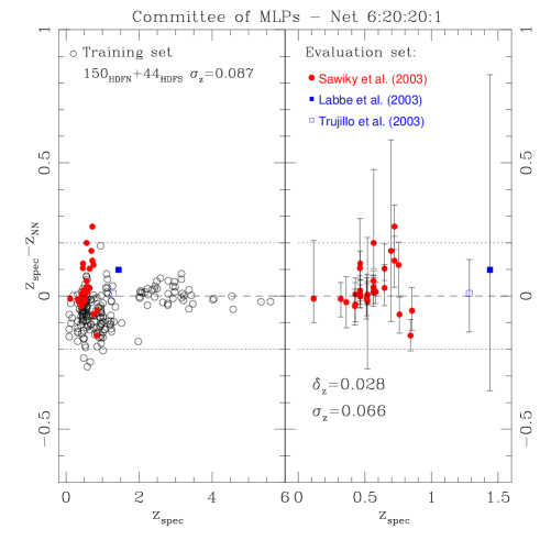
It is interesting to note that the spectroscopic sample in the HDF–S can be used either as a part of the training set or as a validation set in order to calibrate and tune the prediction (at least for the brighter objects) and that with the increasing availability of spectroscopic redshift the prediction can be continually improved. As an example we have used both the HDF–N and the HDF–S spectroscopic samples (194 objects in total) to predict with a 6:20:20:1 architecture the redshifts of $33$ galaxies in the range $0.1<z<1.5$ recently published by Sawicki et al. (2003), Labbé et al. (2003) and Trujillo et al. (2003). The resulting dispersion turns out to be $\sigma_{z}=0.066$ (Fig. 16).

A reference dataset estimating photometric redshifts in the HDF–S down to $I_{AB}\simeq 27$ has been produced: the training has been performed on a set composed of RV00 models, 150 spectroscopic redshifts in the HDF–N and 77 spectroscopic redshifts in HDF–S.

The better generalization obtained using a committee of networks with respect to a single network is more evident in the case of small training sets (Sec. 5.1 and 5.2). If the training set is sufficiently complete and representative, good generalization can be achieved also with a single training.

In summary the NN approach introduces the following advantages:

1. Rapidity in the evaluation phase with respect to more conventional techniques and possibility to deal with very large datasets. The redshifts of $10^{5}$ galaxies can be estimated in few seconds (using a laptop with PIII, 1.1 GHz).

2. The system can quickly learn new information, for example when new spectroscopic redshifts become available.

3. A priori knowledge (such as morphological properties, apparent luminosity, etc.) can be taken into account.

4. There are no assumptions concerning the distribution of the input variables.

5. Feed-forward NNs can also be implemented via hardware, in the so called machine learning scheme. Neural processors have the same generalization and learning ability as the MLP simulated via software (Battiti & Tecchiolli (1995)), but with an extremely high velocity performance ($10^{6-7}$ galaxies per second, a very useful feature in the training phase).

Future developments include a better treatment of photometric errors and upper limits, and the recognition of characteristics of the galaxies (e.g. the type) from the input colors and/or morphological features (such as the $Sersic$ index, luminosity profiles, etc.).