Predictions of mixed non-Gaussian cosmological density fields for the cosmic microwave background radiation

Abstract

We present simulations of the Cosmic Microwave Background Radiation (CMBR) power spectrum for a class of mixed, non-Gaussian, primordial random fields. We assume a skew positive mixed model with adiabatic inflation perturbations plus additional isocurvature perturbations possibly produced by topological defects. The joint probability distribution used in this context is a weighted combination of Gaussian and non-Gaussian random fields, such as: P($\delta$) = (1-$\alpha$)f₁($\delta$) + $\alpha$f₂($\delta$), where f₁($\delta$) is a Gaussian distribution, f₂($\delta$) is a non-Gaussian general distribution, and $\alpha$ is a scale dependent mixture parameter. Results from simulations of CMBR temperature and polarisation power spectra show a distinct signature for very small deviations ($\mathrel{\hbox{\raise 2.15277pt\hbox{$<$}\hbox to0.0pt{\hss\lower 2.15277pt\hbox{$\sim$}}}}$ 0.1%) from a pure Gaussian field. We discuss the main properties of such mixed models as well, their predictions and suggestions on how to apply them to small scale CMBR observations. A reduced $\chi^{2}$ test shows that the contribution of an isocurvature fluctuation field is not ruled out in actual CMB observations, even in WMAP first-year sky map.

1 Introduction

One of the main goals of cosmology today is to determine the origin of primordial density fluctuations. Since CMBR carries the intrinsic statistical properties of cosmological perturbations, it is considered the most powerful tool to investigate the nature of cosmic structure. Tests for Gaussianity of CMBR anisotropy can discriminate between various cosmological models for structure formation.

The most accepted model for structure formation assumes initial quantum fluctuations created during inflation and amplified by gravitational effects. The standard inflation model predicts an adiabatic uncorrelated random field with a nearly flat, scale-invariant spectrum on scales larger than $\sim$ 1-2^∘ (Guth 1981; Salopek, Bond & Bardeen 1981; Bardeen, Steinhardt & Turner 1983). Simple inflationary models also predict the random field follows a nearly-Gaussian distribution, where just small deviations from Gaussianity are allowed (e.g. Gangui et al. 1994). However, larger deviations are also possible in a wide class of alternative models like non standard inflation models with a massless axion field (Allen, Grinstein & Wise 1987); with multiple scalar fields (Salopek, Bond & Bardeen 1981); with a massive scalar field (Koyama, Soda & Taruya 1999); with variations in the Hubble parameter (Barrow & Coles 1990). Cosmic defects models (Kibble 1976; Magueijo & Brandenbergher 2000) also predict the creation of non-Gaussian random fields. In hybrid inflation models (Battye & Weller 1998; Battye, Magueijo & Weller 1999), structure is formed by a combination of (inflation-produced) adiabatic and (topological defects induced) isocurvature density fluctuations. The topological defects are assumed to appear during the phase transition that marks the end of the inflationary epoch. In this scenario, the fields are uncorrelated, combined by a weighted average and obey a non-Gaussian statistics.

The interest in non-Gaussian structure formation models is not unjustified. Indeed, the increasing number of galaxies observed at high redshifts clearly disfavors standard inflationary models with Gaussian initial conditions, which predict these objects should be very rare in the universe (e.g. Weymann et. al. 1998). In addition, statistical evidence for a small level of non-Gaussianity in the anisotropy of CMBR has been found in the COBE/DMR four-year sky maps (Ferreira, Magueijo & Górski 1998) and in the WMAP first-year observations (Chiang et al. 2003). On the other hand, recent CMBR anisotropy observations in large (Smoot et al. 1992; Bennett et al. 1996), intermediate (de Bernardis et al. 2000; Hanany et al. 2000) and small angular scales (Halverson et al. 2002; Stompor et al. 2001; Mason et al. 2002; Pearson et al. 2002; Peiris et al. 2003; Kogut et al. 2003) seem to be in reasonable agreement with inflation predictions. Hence, it is hard to either accept or rule out the non-Gaussian contribution to structure formation.

Actually, if one looks at all the available data, one possible interpretation suggests an intermediate situation where realistic initial conditions for structure formation have small but significant departures from Gaussianity. A scenario in which the details of such departures are understood and calculated may offer a new alternative for evolution of cosmological perturbations (for a present overview, see e.g. Gordon 2001; Gordon et al. 2001) and formation of structures in the Universe. Hopefully, with the improved quality of CMBR observations both on the ground and on board stratospheric balloons, and with data coming from MAP and PLANCK satellites missions (Tauber 2000; Wright 2000) in a very near future, we will possibly be able to unveil the statistical properties of the density field with good precision. This will finally allow us to choose, among the large number of available candidates, the cosmological models that adequately fit the observational data.

In this work, we explore the hypothesis that the initial conditions for structure formation do not necessarily build a single, one-component random field, but a weighted combination of two or more fields. In particular, we are interested in simple mixtures of two fields, one of them being a dominant Gaussian process. In a previous work, Ribeiro, Wuensche & Letelier (2000) (hereafter RWL) used such a model to probe the galaxy cluster abundance evolution in the universe and found that even a very small level of non-Gaussianity in the mixed field may introduce significant changes in the cluster abundance rate. Now, we investigate the effects of mixed models in the CMBR power spectrum, considering a general class of finite mixtures and always combining a Gaussian with a second field to produce a positive skewness density fluctuation field. For this combination we adopt a scale dependent mixture parameter and a power-law initial spectrum, $P(k)=Ak^{n}$. CMBR temperature and polarisation power spectra are simulated for a flat $\Lambda$-CDM model, while varying some cosmological parameters, and the temperature fluctuations are estimated. We show how the shape and amplitude of the fluctuations in CMBR are dependent on such mixed fields and how we can distinguish a standard adiabatic Gaussian field from a mixed non-Gaussian field.

This paper is organised as follows: in the next section, we discuss the main properties of the mixed models. In section 3, we present the simulations results for a standard cosmological $\Lambda$-CDM model mixing Gaussian, lognormal, exponential, Maxwellian and Chi-squared distributions. Simulations for different combinations of cosmological parameters are presented in section 4. In section 5, we finally summarise and discuss the possibilities of use of the proposed mixed composition model for parameter estimation in future small scale CMBR observations.

2 General Description

2.1 Non-Gaussian Random Fields

The use of statistical methods to describe the structure formation process in the universe is due to the lack of complete knowledge about the density fluctuation field $\delta({\bf x})$ at any time $t$. This lead us to treat $\delta({\bf x})$ as a random field in the 3D-space and to assume the universe as a random realization from a statistical ensemble of possible universes. In general, it is possible to assure Gaussianity to this field by simply invoking the central limit theorem (CLT). However, in order to better understand the process of structure formation, it is necessary to investigate the existence and (in case it exists) contribution of non-Gaussian effects to the primordial density field.

Non-gaussianity implies an infinite range of possible statistical models. Hence, the usual approach to this subject is to examine specific classes of non-Gaussian fields. The general procedure to create a wide class of non-Gaussian models is to admit the existence of an operator which transforms Gaussianity into non-Gaussianity according to a specific rule. For a small level of non-Gaussianity, the perturbation theory works well for the density field. For instance, we can define a zero-mean random field $\psi$ which follows a local transformation $\mathcal{F}$ on a underlying Gaussian field:

$$\psi({\bf x})=\mathcal{F}[\phi]\equiv\alpha\phi({\bf x})+\epsilon{(\phi^{2}({\bf x})-\langle\phi^{2}({\bf x})\rangle)}$$ (1)

where $\alpha$ and $\epsilon$ are free parameters of the model. In the limit $\alpha\rightarrow 0$, $\psi$ is chi-squared distributed, while for $\epsilon\rightarrow 0$ one recovers the Gaussian field. The field described by $\psi$ is physically motivated in the context of non-standard inflation models (e.g. Falk et al. 1993; Gangui et al. 1994). Besides, transformation (1) may be considered as a Taylor expansion of more general non-Gaussian fields (e.g. Coles & Barrow 1987; Verde et al. 2000). We also should note that $P(\phi)$ is a Gaussian PDF, while $P(\psi)=\int W(\psi|\phi)P(\phi)\;d\phi$, where $W(\psi|\phi)$ is the transition probability from $\phi$ to $\psi$ (e.g. Taylor & Watts 2000; Matarrese, Verde & Jimenez 2000).

An alternative approach to study non-Gaussian fields is that proposed by RWL, in which the PDF itself is modified as a mixture: $P(\psi)=\alpha f_{1}(\phi)+(1-\alpha)f_{2}(\phi)$, where $f_{1}(\phi)$ is a (dominant) Gaussian PDF and $f_{2}(\phi)$ is a second distribution, with $\alpha$ being a parameter between 0 and 1. This parameter gives the absolute level of Gaussian deviation, while $f_{2}(\phi)$ modulates the shape of the resultant non-Gaussian distribution. The particular choice of RWL was to define $f_{2}$ as a lognormal distribution. Instead of supporting this model with a specific inflation picture, the authors take the simple argument that the real PDF of the density field cannot be strongly non-Gaussian (from COBE data constraints, see Stompor et al. 2001, and from WMAP, see Komatsu et al. 2003) and, at the same time, it should be approximately log-normal in the non-linear regime (from Abell/ACO clusters data, see Plionis & Valdarnini 1995). Indeed, Coles & Jones (1991) argued that the lognormal distribution provides a natural description for the density fluctuation field resulting from Gaussian initial conditions in the weakly non-linear regime. Hence, RWL envisage $\alpha$ as a function of time which turns a nearly Gaussian PDF at recombination ($\alpha\approx 1$) into a nearly lognormal distribution ($\alpha\approx 0$) over the non-linear regime. The problem of taking a direct relationship between the PDF at two different times is not considered by RWL, but it could be done in the context of the extended perturbation theory (Colombi et al. 1997). It is important to note that a mixture of distributions including a lognormal component implies the existence of a non-perturbative contribution of type $e^{\phi}$ in the primordial density field, such that the transformation $\mathcal{F}$ becomes:

$$\psi({\bf x})=\mathcal{F}[\phi]=\alpha\phi({\bf x})+(1-\alpha)e^{\phi({\bf x})}$$ (2)

The physics of the field described by $\psi$ is studied elsewhere (Ribeiro et al. 2003). Here, in continuity of the work of RWL, we investigate the implications of mixed models for the CMBR power spectrum. We take the attitude that, in face of the difficulties to completely describe the primordial density field and its evolution, it is valid to take the predictions of a tentative model like RWL and compare them with observations. Our primary aim is just to find a successful and simple idealization for observed phenomena. Next, we describe the technical details of the mixed models and how to use them to make predictions for the CMBR.

2.2 The Mixed Models

A Gaussian random field is one in which the Fourier components $\delta_{k}$ have independent, random and uniformly distributed phases. In this case, the probability density function in Fourier Space is:

$$P[\delta_{k}]~{}\propto~{}{\rm exp}~{}\left(-{1\over 2}\sum_{k}{|\delta_{k}|^{2}\over\sigma_{k}^{2}}\right)$$ (3)

Such a condition means that the phases are non-correlated in space and assures the statistical properties of the Gaussian fields are completely specified by the two-point correlation function or, equivalently, by its power spectrum $P(k)=|\delta_{k}|^{2}$, which contain information about the density fluctuation amplitude of each scale k. In an isotropic and homogeneous Universe, $k$ represents only the wavevector amplitude.

In the mixed scenario, we suppose that the field has a probability density function of the form:

$$P[\delta_{k}]~{}\propto~{}(1-\alpha)f_{1}(\delta_{k})+\alpha f_{2}(\delta_{k})$$ (4)

In general, the PDF of the Fourier components P$[\delta_{k}]$ is not equal to the PDF of the field P$[\delta]$. However, we can always consider a non-gaussian distribution field like a combination of a gaussian and a non-gaussian distribution. This means that a mixed distribution can be applied to even real and Fourier space in a non-gaussian context, but this not mean that the real and Fourier space have the same kind of combination. In the mixed context, the Fourier components $\delta_{k}$ have only a small fraction of correlated phase in space represented by the second distribution. The first field will always be the Gaussian component and a possible effect of the second component is to modify the Gaussian field to have a positive tail. The parameter $\alpha$ in (4) allows us to modulate the contribution of each component to the resultant field. The Gaussian component represents the adiabatic (or isentropic) inflation field and the second component may represent the effect of adding an isocurvature field produced due to some primordial mechanism acting on the energy distribution, such as topological defects. The two component random field can be generated by taking $\delta_{k}=P(k)\nu^{2}$, where $\nu$ is a random number with distribution given by (4). Then, the mean fluctuation, $\langle\delta^{2}(x)\rangle$, is proportional to:

$$\int_{k}P(k)\left[\int_{\nu}[(1-\alpha)f_{1}(\nu)+\alpha f_{2}(\nu)]\nu^{2}\;d\nu\right]\;d^{3}k$$ (5)

The primordial power spectrum of the mixed field has the form:

$$P(k)^{mix}\equiv M^{mix}(\alpha)P(k)$$ (6)

where the $P(k)$ represents a power-law spectrum and M^mix($\alpha$) is the mixture term, which account for the statistics effect of a new component, a functional of $f_{\mathit{1}}$ and $f_{\mathit{2}}$:

$$M^{mix}(\alpha)\equiv\int_{\nu}[(1-\alpha)f_{1}(\nu)+\alpha f_{2}(\nu)]\nu^{2}\;d\nu$$ (7)

Resolving this integral assuming $f_{1}$ as the Gaussian distribution, the mixture term is:

$$M^{mix}(\alpha)=1-\alpha+\alpha\int_{\nu}f_{2}(\nu)\nu^{2}\;d\nu$$ (8)

In this work, we explore the case of a positive skewness model, where the second field adds to the Gaussian component a positive tail representing a number of rare peaks in the density fluctuation field. To represent the effect of adding an isocurvature field we have chosen the well-known lognormal, exponential, Rayleigh, Maxwellian and Chi-squared distributions as the second component. These random fields have already been used to calculate the size and number of positive and negative peaks in CMBR distribution, under the assumption that it possesses a single, non-Gaussian, component (Coles & Barrow 1987), but, to our present knowledge, they have never been used in this context of mixed fields.

Like the hybrid inflation models (Battye & Weller 1998; Battye, Magueijo & Weller 1999), mixture models consider the scenario in which structure is formed by both adiabatic density fluctuations produced during inflation and active isocurvature perturbations created by cosmic defects during a phase transition which marks the end of inflationary epoch. Nevertheless, the mixed scenario considers a possible correlation between the adiabatic and the isocurvature fields only on the post-inflation Universe. So, the fluctuations in super-horizon scales are strictly uncorrelated. While the hybrid inflation scenario considers the super and sub-degree scales of CMBR anisotropy due to uncorrelated strings and inflation fields, the mixed model considers an effective mixed correlated field acting inside the Hubble horizon, in sub-degree scales. To allow for this condition and keep a continuous mixed field, the mixture parameter was defined as a scale dependent parameter, $\alpha$ $\equiv$ $\alpha$(k). The simplest choice of $\alpha$(k) is a linear function of $k$:

$$\alpha(k)\equiv\alpha_{0}k$$ (9)

In this case, the mixture term is a function of $k$, $M(\alpha_{0}$, $k$), and the mixed primordial power spectrum is:

$$P(k)^{mix}\equiv M^{mix}(\alpha_{0},\textit{k})P(k)$$

$$=k^{n}+M(\alpha_{0})k^{n+1}$$ (10)

where M($\alpha$₀) represents only the coefficient dependence, $\alpha$₀. In the case of a pure Gaussian field, $\alpha$₀ $\approx$ 0, and the mixed power spectrum will be a simple power-law spectrum. In the case of a mixed field, the phase correlations between both fields are estimated by the integral in Eq. (8), on mixture scales defined by Eq. (9).

3 Mixed Non-Gaussian Fields in the Cosmic Microwave Background Radiation

Since radiation and matter were tightly coupled up to $3\times 10^{5}$ years, understanding the statistical properties of the CMBR can be an extremely powerful tool to investigate the Gaussian nature of the cosmological density fluctuations field. Comparing theoretical predictions and observational data, it is possible to select the models that account for the best description of the temperature field. The statistical nature of the initial conditions is a basic assumption of an algorithm to generate CMBR power spectra. In this work, instead of assuming the usual Gaussian initial condition, we analyze the consequences of using mixed (non-Gaussian) initial conditions to generate CMBR power spectra.

To estimate a CMB temperature power spectrum, we need to evaluate the evolution of fluctuations generated in the early universe through the radiation-dominated era and recombination. In a mixed model with a small deviation from Gaussianity (i.e. possible small fraction of correlated phases in space), we can, for simplicity, ignore the coupled phase evolution through the radiation-dominated era and consider only the evolution of the amplitude of the Fourier modes within the framework of linearized perturbation theory. Following this approach, the evolution of both adiabatic and isocurvature components of the mixed density field is considered as an independent process. Only their effective amplitude correlation is considered at the Last Scattering Surface (LSS) of the photons from CMBR. To compute the independent evolution, we have used the Linger function of the COSMICS code package (Bertschinger 1999) for an adiabatic $\Lambda$-CDM mode and an isocurvature $\Lambda$-CDM mode. The Linger function integrates the coupled, linearized, Einstein, Boltzmann, and fluid equations governing the evolution of scalar metric perturbations and density perturbations for photons, baryons and cold dark matter in a perturbed flat Robertson-Walker universe, in a synchronous gauge. Linger does generate the photon density field to compute the CMBR anisotropy.

To allow for a possible coupling of both fields in the last scattering surface, the CMBR temperature and polarization power spectra were estimated by a mixed photon density function incorporated to the original COSMICS package in estimation of the multipole moments, C_l:

$$C_{l}=4\pi\int_{0}^{k_{max}}\;d^{3}kP^{mix}(k)(\Delta_{l}^{mix})^{2}(k,\tau)$$ (11)

The function $\Delta_{l}^{mix}$ represents the mixed photon density field in the last scattering surface defined by:

$$\Delta_{l}^{mix}\equiv(1-\alpha_{0}k)\Delta_{l}^{Adi}+\alpha_{0}k\Delta_{l}^{Iso}$$ (12)

where $\Delta_{l}^{mix}$ and $\Delta_{l}^{Iso}$ are the photon density function estimated by COSMICS, respectively, for an adiabatic and an isocurvature seed initial conditions.

Since we are not considering the correlation between modes in different scales (while we are considering just linear evolution) the amplitude of the mixed field is obtained by the moment:

$$\langle\Delta_{l}^{mix}(k)\Delta_{l}^{mix}(k)^{*}\rangle=\langle|\Delta_{l}^{mix}|^{2}\rangle=\langle|\Delta_{l}^{Adi}|^{2}+$$

$$\ \alpha_{0}^{2}k^{2}(|\Delta_{l}^{Iso}|^{2}+|\Delta_{l}^{Adi}|^{2}-2|\Delta_{l}^{Iso}||\Delta_{l}^{Adi}|)+$$

$$2\alpha_{0}k|\Delta_{l}^{Adi}||\Delta_{l}^{Iso}|-2\alpha_{0}k|\Delta_{l}^{Adi}|^{2}\rangle$$

which contains correlated terms between the amplitudes of the adiabatic and the isocurvature fields, and not only the independent contribution of each field. The coefficients of the amplitudes appearing on the second and third line of Eq. (13) represent the mixing effect between the fields and the mixing parameter $\alpha$₀ controls the contribution of the isocurvature field relative to the adiabatic field. Since we are not considering independent fields amplitudes and we also consider a possible small fraction of phase correlation, we can describe this mixed field by a non-gaussian statistics like Eq. (4).

Inserting (13) in (11), we have a mixed term in the C_l estimation. This condition suggests that the amplitude of both fields are cross-correlated at the LSS, with a mixing ratio defined by $\alpha$₀ and in a characteristic scale defined by $\alpha$₀k. The power spectra estimated by Eq. (11) consider a flat $\Lambda$-CDM universe distorted by a non-gaussian statistics, with constant spectral index in the range of 0.8 $\leq$ n $\leq$1.2. In a case of a pure gaussian field, $\alpha$₀=0, we obtain only the first term of the power law spectrum in Eq. (10), for a pure and non-correlated adiabatic field, the first term in Eq. (13), described only by a gaussian distribution.

In this section we present the simulations of the CMBR temperature and polarization power spectra for the present standard $\Lambda$-CDM model (H₀= 70Km/sMpc; $\Omega$₀ = 1; $\Omega$_bh² = 0.03, $\Omega$_CDMh² = 0.27, $\Omega$_Λh² = 0.7 and n =1.1). Another set of simulations, using different values for the above parameters, is presented in Section 4. Figure 1 contains the mixed (Gaussian-lognormal) CMBR temperature power spectrum estimated for different values of $\alpha$₀. The temperature fluctuations are normalized by the RMS quadrupole amplitude estimated by the COBE/DMR experiment, Q_rms=( 13 $\pm$ 4) $\mu$K (Smoot et al. 1992). Figure 2 shows the mixed (Gaussian-lognormal) polarization power spectrum.

Figure 1: CMBR temperature mixed angular power spectrum estimated for a standard $\Lambda$-CDM model in different mixing degrees.

Figure 2: CMBR polarization mixed angular power spectrum estimated for a standard $\Lambda$-CDM model in different mixing degrees.

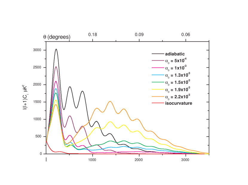
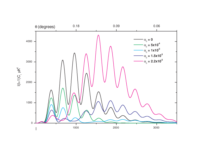
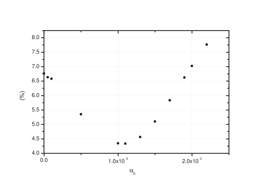
In Figures 1 and 2, we see how the shape and amplitude of the spectrum change even for small values of $\alpha$_o ($\sim$10^-4-10^-3). The peaks intensity are clearly susceptible to the existence of mixed fields, although distinguishing peaks of higher order (2^nd, 3^rd, etc.) in the mixed context is not a straightforward task, since their intensity, compared to the first peak, are very low. But, on the other hand, it is very clear how the peaks intensity changes while the mixture increases. The effect of increasing $\alpha$₀ is a power transfer to smaller scales (l >1000), while the super-degree scales are not affected. According to our definition, the effect of $\alpha$(k) upon the fields can be seen only inside the Hubble horizon. In Figure 3, we see that the fraction of the CMBR polarized component depends on the mixture parameter and ranges from 4.3 to 7.7% of the total intensity for 10^-4$\leq$ $\alpha$₀ $\leq$10^-3.

We consider the relation between the peaks’ intensity and $\alpha$₀ a key result of this work, since it is a prediction of the mixed model that can be easily tested and, moreover, offers a good and straightforward tool to be applied to the forthcoming data sets from present CMBR experiments and WMAP and PLANCK satellites. Both of them will map the CMBR power spectrum in the $l-$interval studied in this paper and the data from the above mentioned experiments will surely offer a good bench test for this model.

To illustrate the mean properties of the CMBR mixed fluctuations field, we have estimated the mean temperature fluctuations, ($\Delta$T/T)_rms:

$$\left({\Delta T\over T}\right)_{rms}^{2}={1\over 4\pi}\sum_{l=2}{(2l+1)C_{l}}$$ (14)

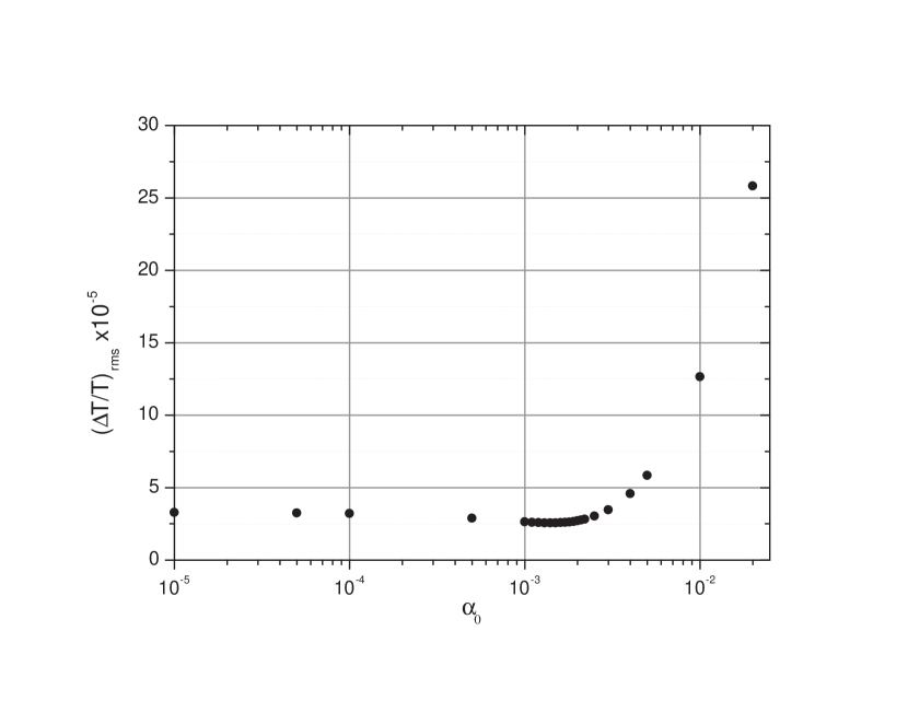
The behaviour of ($\Delta$T/T)_rms for the Gaussian-lognormal mixture is shown in Figure 4. For large values of $\alpha$₀ ($\alpha$₀>3x10^-3) we see a fast increase in the temperature fluctuations, probably caused by correlation excess between the mixed fields, resulting in more power in small scales. From these results, we can set an acceptable range for $\alpha_{0}$ to be $\alpha_{0}\lesssim 3\times 10^{-3}$.

Figure 3: CMBR polarized component simulated for a mixed Gaussian-lognormal model in a standard combination of cosmological parameters.

Figure 4: CMBR mean fluctuation temperature estimated for a Mixed Gaussian-lognormal model in a standard combination of cosmological parameters.

In Table 1, we present the mean temperature fluctuations ($\Delta$T/T)_rms estimated for different values of $\alpha$₀ for mixtures between Gaussian, Exponential, lognormal, Maxwellian and Chi-squared with one degree of freedom distributions. For a Rayleigh distribution, the integral in equation (8) has the same value of the integral for a exponential distribution. So, the mixed Gaussian-exponential and the Gaussian-Rayleigh power spectrum are exactly the same. As we can see in Table 1, the difference between various mixture components is quite small for the mixed models, due to a very small change in P^mix for different components. For $\alpha$₀$\sim$10^-3, the mixed term, M($\alpha$₀), is about 10^-3. To obtain C_l we have to multiply M($\alpha$_o) by kⁿ⁺¹ ($\sim$10^-1)ⁿ⁺¹ and integrate in dk. So, the difference in C_l due to different mixture components is about $\sim$10^-4-10^-5, too small compared to the simulations errors ($\sim$10^-3) for C_l estimation in $\mu K^{2}$. However, the difference between a mixed non-Gaussian and a pure Gaussian field is evident in both temperature and polarization CMBR power spectra. It is clearly seen that the amplitude fluctuations change with the mixture parameter $\alpha$₀, but the main ingredient of the model seems to be the mixed (correlated) photon density field considered in the last scattering surface, and not only the statistic treatment of the phase correlation introduced in P^mix. A practical way to discriminate between a pure Gaussian (adiabatic) field and a mixed non-Gaussian one is comparing the polarized component, the mean temperature fluctuations and the peaks amplitude in the power spectrum.

($\Delta$T/T)_rms x10^-5
$\alpha_{0}$ $G+Exp$ $G+Ln$ $G+Max$ $G+\chi^{2}$ 0 3.2941 3.2941 3.2942 3.2942 1.0E-05 3.2848 3.2847 3.2848 3.2848 5.0E-05 3.2478 3.2478 3.2480 3.2480 1.0E-04 3.2028 3.2027 3.2028 3.2028 5.0E-04 2.8850 2.8850 2.8850 2.8850 1.0E-03 2.6250 2.6247 2.6251 2.6251 1.3E-03 2.5603 2.5595 2.5605 2.5605 1.5E-03 2.5591 2.5579 2.5594 2.5593 1.7E-03 2.5915 2.5899 2.5919 2.5919 1.9E-03 2.6564 2.6543 2.6569 2.6568 2.1E-03 2.7517 2.7487 2.7519 2.7518 2.5E-03 3.0184 3.0195 3.0195 3.0193 5.0E-03 5.8409 5.8323 5.8433 5.8422 1.0E-02 12.6310 12.6413 12.6417 12.6371 6.0E-02 62.4921 62.7690 62.7797 62.6557 1.0E-01 79.8232 80.3811 80.4025 80.1531

Table 1: The mean temperature fluctuations, $(\Delta T/T)_{rms}\times 10^{-5}$, estimated for some mixture components normalised by COBE.

Multicomponent models resulting in an excess of power in small scales have already been investigated with the aid of CMBR anisotropy simulations. For instance, Bucher et al. (2000) have investigated two CDM isocurvature modes (with a neutrino isocurvature and an isocurvature velocity perturbations), evaluated by the linearized perturbation theory in distinct regular and singular modes (rather than growing and decaing modes), and have found a great variation of peaks intensity for a different initial power spectra. Another approach of multicomponent models is that of Gordon (2001) and Amendola et al (2002).They consider a correlated field of adiabatic and isocurvature perturbations produced during a period of cosmological inflation, described in a generic power law spectrum, and show that correlations can cause the acoustic peak height to increase relative to the plateau of CMBR.

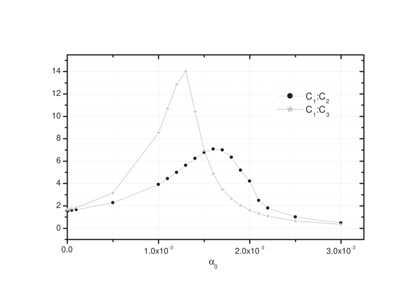
Our point is quite different of those from the above mentioned authors. We show that it is possible to directly assess and quantify the mixture of a correlated adiabatic and isocurvature non-Gaussian field. Figure 5 shows the relative amplitude of the most distinguished peaks (the first three peaks) for a Gaussian-lognormal mixed model temperature power spectrum. This plot clearly shows the difference in the relative amplitude of the peaks for $\alpha$₀ < 3x10^-3. This behaviour points to another possibility to extract information from a CMBR power spectrum: the possibility of detecting weakly mixed density fields, even if we can not exactly identify the mixture components distribution.

Figure 5: The relative amplitude of the first three peaks for a Gaussian-lognormal mixed model temperature power spectrum. $C_{i}:C_{j}$ means the ith peak amplitude divided by the jth peak amplitude.

4 Mixed Models and Cosmological Parameters

A key question that will possibly be asked when trying to apply this model to CMBR measurements is whether we can distinguish the effects of a mixed field from those of variations in the cosmological parameters. In order to answer this question and quantify how a given cosmological parameter variation modify the properties of an a priori unknown mixed field, we ran a number of realisations for a wide range of cosmological parameters values, for both pure Gaussian and mixed fields.

CMBR observational data are in good agreement with the basic preferences of standard inflation scenarios: flat geometry ($\Omega$_tot $\sim$ 1) and a nearly scale invariant primeval spectrum (n $\sim$ 1). Nevertheless, degeneracies in parameter space prevent independent determination of various cosmological parameters, like $\Omega$_b, (the baryon density energy), $\Omega$_CDM, (cold dark matter energy density), $\Omega$_Λ (vacuum energy density) and H₀ (the Hubble constant) (Turner 1998; Efstathiou 2001). Recent CMBR and large scale structure observations suggest the Hubble constant H₀ to assume values in the range (60 < H₀ < 70)(65$\pm$5) km/sec.Mpc (Turner 1998); and a positive cosmological constant value in the range (0.065< $\Omega$_Λ <0.85) (Efstathiou 2001; Spergel et al. 2003). The mass density of baryons determined by Big Bang nucleossinthesys is $\Omega$_b =(0.019 $\pm$ 0.01)h^-2, which is in good agreement with CMBR observations (Stompor et al. 2001). To be consistent with these estimations, we ran another set of realizations for a pure adiabatic Gaussian field, considering a flat Universe and a range of possibilities for five cosmological parameters: 0.8< n <1.2; 0.015 <$\Omega$_b< 0.03; 0.6 <$\Omega$_Λ< 0.8; and 60 <H₀< 80. The cold dark matter density was set as 1-($\Omega$_b + $\Omega$_Λ), ranging of 0.170 < $\Omega$_cdm< 0.385. The temperature power spectra, simulated for a pure Gaussian field generated with the above range of parameters are plotted in Figures 6 and 7.

Figure 6: The temperature power spectra simulated for a pure Gaussian field combining a wide class of cosmological parameters. In A, the curves show variations in the Hubble constant for a model with $\Omega_{b}=0.03$, $\Omega_{cdm}=0.27$, $\Omega_{\Lambda}=0.7$ and $n=1.1$. In B, C, and D, $\Omega_{b}$ is set as 0.015, 0.023 and 0.03, respectively; $\Omega_{cdm}$ and $\Omega_{\Lambda}$ is varying, while the spectral index is fixed as 1.1, and $H_{0}=70$.

Figure 7: The temperature power spectra simulated for a pure Gaussian field for a model with $\Omega_{b}=0.03$, $\Omega_{cdm}=0.27$, $\Omega_{\Lambda}=0.7$, $H_{0}=70$ and spectral index varying from 0.8 to 1.2.

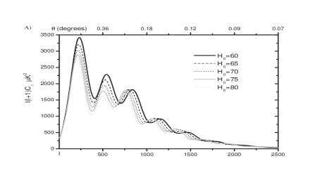
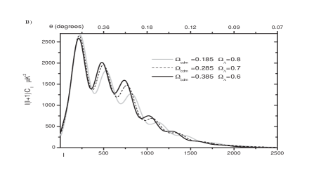
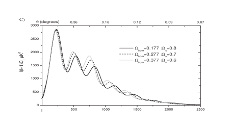
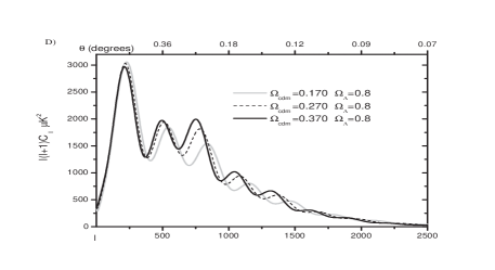
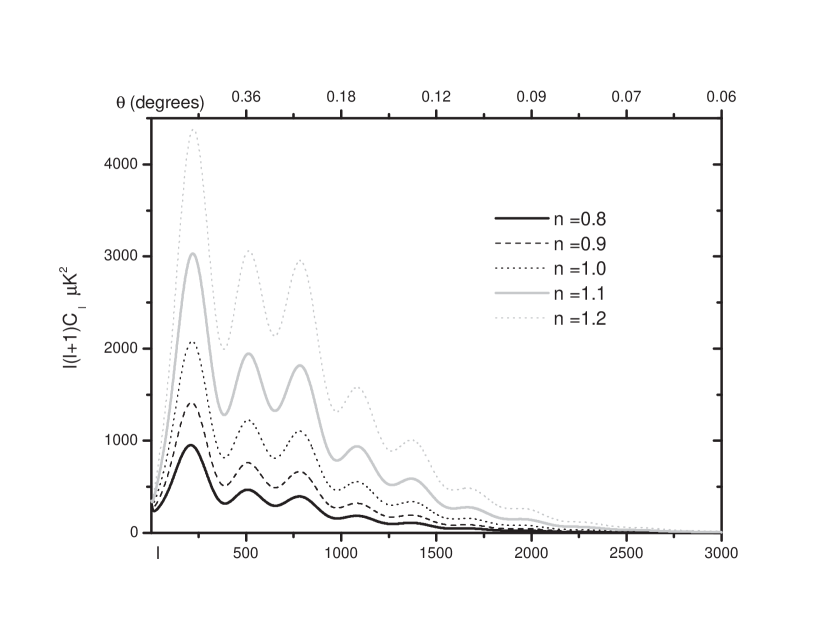
We can see the effect of variations in the Hubble parameter in in Figure 6A. Increasing H₀, the position of all peaks are deviated towards smaller l while their amplitudes decrease. For fixed $\Omega$_b, the effect of increasing $\Omega$_cdm while reducing $\Omega$_Λ is to shift the second and third acoustic peaks positions to smaller l and to higher amplitudes, while the primary peak features are barely disturbed. The first peak has lower intensity for high $\Omega$_cdm (and low $\Omega$_Λ), while higher order peaks have higher intensity, as can be seen in Figures 6B, 6C and 6D. Figure 7 shows the effect of varying the spectral index, n, in a pure adiabatic Gaussian field. As n increases, all the acoustic peaks become intensified and slightly shifted to smaller l.

For all the combined cosmological parameters simulated we have estimated the relative amplitude of the first three acoustic peaks and the mean temperature fluctuation. The estimated values are presented in Table 2. Comparing the values presented in Table 2 with the curves shown in Figure 6, we observe that the relative amplitude of the peaks is lower than 2.1 for a wide combination of cosmological parameters, while the relative amplitude is greater than 2, for a mixed degree in the range: 5x10^-4< $\alpha$₀ <2.1x10^-3. So, comparing the peaks amplitude, a mixed (adiabatic and isocurvature) spectrum is clearly distinct from a pure adiabatic one with a different combination of cosmological parameters.

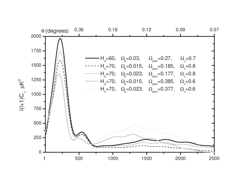
Figure 8 shows the behavior of temperature power spectrum for mixed models according to the variations in the cosmological parameters values, for five different cosmological models with $\alpha$₀=1.5x10^-3. The behaviour of the acoustic peaks is similar to that seen in Figure 1, with power being transfered to higher l, while the super-degree scales are not affected. Table 3 contains the relative amplitude of the peaks and the mean temperature fluctuation for the seventeen simulated mixed models, using $\alpha$₀=5x10^-4.

${\rm Model}$	$C_{1}:C_{2}$	$C_{1}:C_{3}$	$(\Delta T/T)rms$
			$\times 10^{-5}$
$H_{0}$=70 $\Omega_{b}$=0.015
$\Omega_{\Lambda}$= 0.8 n= 1.1	1.46	2.09	3.057
$H_{0}$=70 $\Omega_{b}$=0.015
$\Omega_{\Lambda}$= 0.7 n= 1.1	1.35	1.79	3.121
$H_{0}$=70 $\Omega_{b}$=0.015
$\Omega_{\Lambda}$= 0.6 n= 1.1	1.28	1.62	3.148
$H_{0}$=70 $\Omega_{b}$=0.023
$\Omega_{\Lambda}$= 0.8 n= 1.1	1.54	1.95	3.157
$H_{0}$=70 $\Omega_{b}$=0.023
$\Omega_{\Lambda}$= 0.7 n= 1.1	1.43	1.66	3.221
$H_{0}$=70 $\Omega_{b}$=0.023
$\Omega_{\Lambda}$= 0.6 n= 1.1	1.37	1.49	3.255
$H_{0}$=70 $\Omega_{b}$=0.030
$\Omega_{\Lambda}$= 0.8 n= 1.1	1.65	1.98	3.226
$H_{0}$=70 $\Omega_{b}$=0.030
$\Omega_{\Lambda}$= 0.7 n= 1.1	1.56	1.67	3.295
$H_{0}$=70 $\Omega_{b}$=0.030
$\Omega_{\Lambda}$= 0.6 n= 1.1	1.50	1.49	3.326
$H_{0}$=60 $\Omega_{b}$=0.030
$\Omega_{\Lambda}$= 0.7 n= 1.1	1.50	1.88	3.454
$H_{0}$=65 $\Omega_{b}$=0.030
$\Omega_{\Lambda}$= 0.7 n= 1.1	1.51	1.76	3.368
$H_{0}$=75 $\Omega_{b}$=0.030
$\Omega_{\Lambda}$= 0.7 n= 1.1	1.63	1.61	3.226
$H_{0}$=80 $\Omega_{b}$=0.030
$\Omega_{\Lambda}$= 0.7 n= 1.1	1.73	1.57	3.170
$H_{0}$=70 $\Omega_{b}$=0.030
$\Omega_{\Lambda}$= 0.7 n= 0.8	2.03	2.40	2.004
$H_{0}$=70 $\Omega_{b}$=0.030
$\Omega_{\Lambda}$= 0.7 n= 0.9	1.86	2.12	2.349
$H_{0}$=70 $\Omega_{b}$=0.030
$\Omega_{\Lambda}$= 0.7 n= 1.0	1.70	1.88	2.773
$H_{0}$=70 $\Omega_{b}$=0.030
$\Omega_{\Lambda}$= 0.7 n= 1.2	1.43	1.48	3.929

Table 2: The relative amplitude of the peaks and the mean temperature fluctuation estimated for a wide class of models for a pure Gaussian field.

Figure 8: The temperature power spectra simulated for a mixed Gaussian-lognormal field for some classes of $\Omega_{b}$, $\Omega_{cdm}$, $\Omega_{\Lambda}$ and $H_{0}$. The spectral index is set as 1.1, and the mixture degree is $1.5\times 10^{-3}$.

${\rm Model}$	$C_{1}:C_{2}$	$C_{1}:C_{3}$	$(\Delta T/T)rms$
			$\times 10^{-5}$
$H_{0}$=70 $\Omega_{b}$=0.015
$\Omega_{\Lambda}$= 0.8 n= 1.1	2.00	3.64	2.366
$H_{0}$=70 $\Omega_{b}$=0.015
$\Omega_{\Lambda}$= 0.7 n= 1.1	1.91	3.33	2.386
$H_{0}$=70 $\Omega_{b}$=0.015
$\Omega_{\Lambda}$= 0.6 n= 1.1	1.87	3.19	2.391
$H_{0}$=70 $\Omega_{b}$=0.023
$\Omega_{\Lambda}$= 0.8 n= 1.1	2.14	3.44	2.449
$H_{0}$=70 $\Omega_{b}$=0.023
$\Omega_{\Lambda}$= 0.7 n= 1.1	2.07	3.10	2.472
$H_{0}$=70 $\Omega_{b}$=0.023
$\Omega_{\Lambda}$= 0.6 n= 1.1	2.05	2.95	2.503
$H_{0}$=70 $\Omega_{b}$=0.030
$\Omega_{\Lambda}$= 0.8 n= 1.1	2.33	3.51	2.513
$H_{0}$=70 $\Omega_{b}$=0.030
$\Omega_{\Lambda}$= 0.7 n= 1.1	2.29	3.15	2.557
$H_{0}$=70 $\Omega_{b}$=0.030
$\Omega_{\Lambda}$= 0.6 n= 1.1	2.30	2.97	2.587
$H_{0}$=60 $\Omega_{b}$=0.030
$\Omega_{\Lambda}$= 0.7 n= 1.1	2.07	3.32	2.604
$H_{0}$=65 $\Omega_{b}$=0.030
$\Omega_{\Lambda}$= 0.7 n= 1.1	2.16	3.20	2.565
$H_{0}$=75 $\Omega_{b}$=0.030
$\Omega_{\Lambda}$= 0.7 n= 1.1	2.49	3.14	2.547
$H_{0}$=80 $\Omega_{b}$=0.030
$\Omega_{\Lambda}$= 0.7 n= 1.1	2.76	3.18	2.565
$H_{0}$=70 $\Omega_{b}$=0.030
$\Omega_{\Lambda}$= 0.7 n= 0.8	3.00	4.55	1.695
$H_{0}$=70 $\Omega_{b}$=0.030
$\Omega_{\Lambda}$= 0.7 n= 0.9	2.74	4.02	1.930
$H_{0}$=70 $\Omega_{b}$=0.030
$\Omega_{\Lambda}$= 0.7 n= 1.0	2.50	3.55	4.664
$H_{0}$=70 $\Omega_{b}$=0.030
$\Omega_{\Lambda}$= 0.7 n= 1.2	2.11	2.79	2.976

Table 3: The relative amplitude of the peaks and the mean temperature fluctuation estimated for a wide class of models for a mixed Gaussian-lognormal field with a mixed degree of $5\times 10^{-4}$.

Comparing the values in Tables 2 and 3, we can verify the difference between the relative amplitude for mixed and pure models, for a quite large combination of cosmological parameters. It seems clear that the effect of mixed models upon the acoustic peaks amplitude is more pronounced than those achieved through variations of the cosmological parameters in a pure model. Besides that, once the above cosmological parameters are determined with better precision, power spectrum examination can be used to identify a mixed density field and estimate the mixture degree by comparing the peaks intensity.

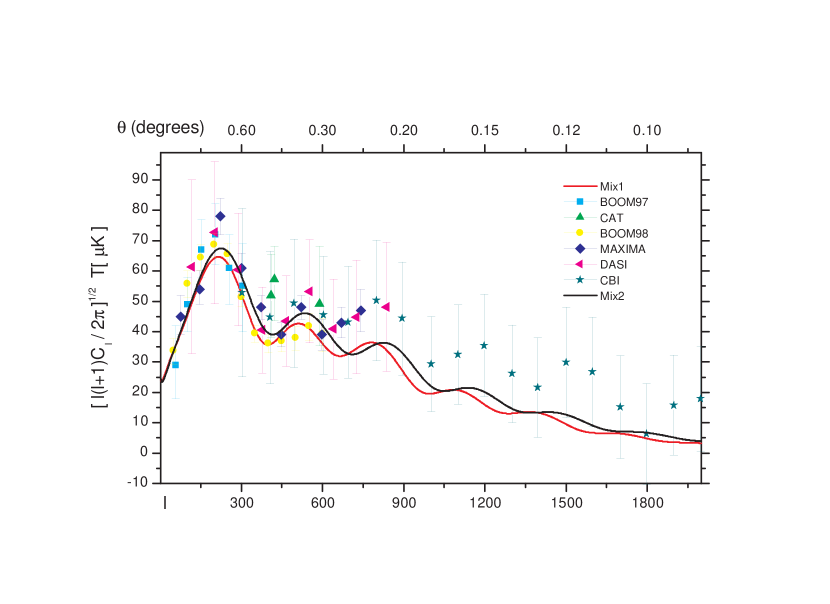
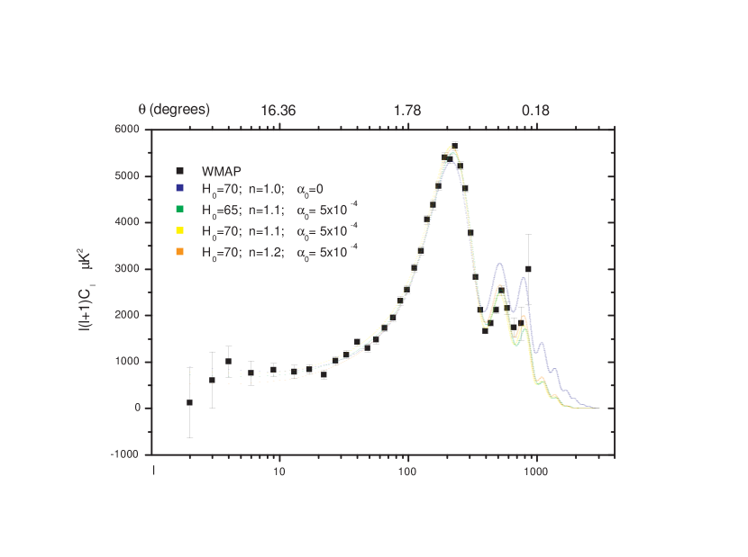
In order to quantify a possible non-gaussian contribution to the fluctuations field, we have made a maximum likelihood approach to power spectrum estimated by several classes of CMB experiments. Our best estimate of the angular power spectrum for the CMB is shown in Figure 9 for a combination of various CMB data prior to WMAP, and, in Figure 10, the best standard gaussian and the bests estimated mixed model fits for the first-year WMAP data. The $\chi^{2}$ test shows that the contribution of an isocurvature fluctuation field is not ruled out in actual CMB observations.

Figure 9: Temperature fluctuation estimated for some classes of CMBR experiments and the mixed model estimative for $\alpha$₀=5x10^-4 in two combinations of cosmological parameters, Mix1: $\Omega_{b}=0.023$, $\Omega_{cdm}=0.177$, $\Omega_{\Lambda}=0.8$; $n=1.1$ and $H_{0}=70km/sMpc$; and Mix2: $\Omega_{b}=0.03$, $\Omega_{cdm}=0.27$, $\Omega_{\Lambda}=0.7$; $n=1.1$ and $H_{0}=70km/sMpc$. The reduced $\chi^{2}$ estimated are 1.010 and 1.000, respectively.

Figure 10: The angular power spectrum estimated for the WMAP mission, the predictions of the standard $\Lambda-CDM$ model and tree best-fit $\Lambda-CDM$ mixed model for the CMBR. In all models illustrated, the best cosmological parameters combination found was: $\Omega_{b}=0.03$, $\Omega_{cdm}=0.27$, $\Omega_{\Lambda}=0.7$. The reduced $\chi^{2}$ estimated are 13.399 for $H_{0}=70km/sMpc$; $n=1.0$ and $\alpha_{0}=0$; 1.723 for $H_{0}=65km/sMpc$; $n=1.1$ and $\alpha_{0}=5\times 10^{-4}$; 2.260 for $H_{0}=70km/sMpc$; $n=1.2$ and $\alpha_{0}=5\times 10^{-4}$ and 2.546 for $H_{0}=70km/sMpc$; $n=1.1$ and $\alpha_{0}=5\times 10^{-4}$.

5 Discussion

Assuming the hypothesis that the initial fluctuation field is the result of weakly correlated adiabatic and isocurvature mixed fields, we made a number of realisations of CMBR temperature and polarisation power spectra and estimated the mean temperature fluctuations combining Gaussian, Exponential, Lognormal, Rayleigh, Maxwellian and a Chi-squared distributions. The contribution of a second field is estimated by the distortion of the power spectrum and is also considered a correlated amplitude for the mixed field. Some important results were obtained. We show that it is possible to directly assess and quantify the mixture of a correlated adiabatic and isocurvature non-Gaussian field. The simulations clearly show the difference in the relative amplitude of the acoustic peaks for a mixed correlated model. This behaviour points to another possibility to extract information from a CMBR power spectrum: the possibility of detecting weakly mixed density fields, even if we can not exactly identify the mixture components distribution. The simulations show that the influence of the specific statistics of the second component in the mixed field is not so important as the cross-correlation between the amplitudes of both fields. This seems to be very important in the CMBR power spectrum estimation. We claim that a physical mechanism responsible for generation of both field could result in a distinctive signature in CMBR. We also show the results are not strongly affected by the choice of the cosmological parameters and hence the characteristic behaviour of the acoustic peaks amplitude and the polarized component can be used as a cosmological test for the nature of the primordial density field. Indeed, the predictions of mixture models are very distinct from the pure density fields, especially for small angular scales.

Also, recent temperature fluctuation CMBR observational data do not rule out a mixture component in a small level of non-Gaussianity, with a mixture coefficient of $\sim\times 10^{-4}$, as can be seen in Figure 9 and Figure 10. With the new generation of the CMBR experiments, especially the expected satellite mission Planck (Tauber 2000), we expect to be able to compare more observations in small scales, with better signal to noise and larger sky coverage, to the predictions of our class of mixed models and estimate the physical mechanisms responsible for structure formation. In despite of the degeneration of the power spectrum for mixed PDF, we expect to better estimate the statistical description of fluctuations in a mixed scenario by carrying out the investigation, in a non-gaussian context, of the average correlation function and the correlation function for high amplitude peaks (Andrade et al., 2003)

References

- (1) Allen T. J., Grinstein B., Wise M. B., 1987, Phys. Lett. B, 197, 66.
- (2) Amendola L. et al., 2002, Phys.Rev.Lett., 88, 211302.
- (3) Andrade A.P.A., Ribeiro A.L.B., Wuesnche C.A., in preparation.
- (4) Bardeen J.M., Steinhardt P.J., Turner M.S., 1983, Phys. Rev.D, 28, 679.
- (5) Barrow J.D., Coles P., 1990, MNRAS, 244, 188.
- (6) Battye R.A., Weller J., 1998, in Montmerle P. J., Auborg E., eds., The 19th Texas Symposium on Relativistic Astrophysics and Cosmology, Paris, France.
- (7) Battye R.A., Magueijo J., Weller J., 1999, astro-ph/9906093.
- (8) Bennett C.L. et al., 1996, ApJ, 464, L1.
- (9) de Bernardis P. et al., 2000, Nature, 404, 955.
- (10) Bertschinger E., 1999, COSMICS: Cosmological Initial Conditions and Microwave Anisotropy Codes, Massachusetts Institute of Technology, (http://arcturus.mit.edu/cosmics).
- (11) Bucher M. et al., 2000, astro-ph/9904231.
- (12) Chiang, LY., Naselsky, P.D., Verkhodanov, O.L., Way, M.J., 2003, astro-ph/0303643.
- (13) Coles P., Barrow J., 1987, MNRAS, 228, 407.
- (14) Coles P., Jones B., 1991, MNRAS, 248, 1.
- (15) Colombi S. et al., 1997, MNRAS, 287, 241.
- (16) Efstathiou G., 2001, MNRAS, astro-ph/0109152.
- (17) Falk T. et al., 1993, ApJ, 403, L1.
- (18) Ferreira P.G., Magueijo J., K.M. Górski, 1998, ApJ., 503, L1.
- (19) Gangui A. et al., 1994, ApJ, 430, 447.
- (20) Gordon, C. et al., 2001, Phys. Rev. D, 63, 23506.
- (21) Gordon, C. Ph.D. Thesis, 2001 and astro-ph/0112523.
- (22) Guth A.H., 1981, Phys. Rev. D, 23, 347.
- (23) Halverson N.W. et al., 2002, ApJ, 568, 38.
- (24) Hanany S. et al., 2000, ApJ, 545, L5.
- (25) Kibble T.W.B., 1976, J. Phys. A, 9, 1387.
- (26) Kogut, A. et al., 2003, astro-ph/0302213.
- (27) Komatsu, E. et al., 2003 astro-ph/0302223.
- (28) Koyama K., Soda J., Taruya A., 1999, MNRAS, 310, 1111.
- (29) Ma C., Bertschinger E., 1995, ApJ, 455, 721.
- (30) Magueijo J., Brandenbergher R. H., 1999, Lecture notes of the International School on Cosmology, Kish Island, Iran.
- (31) Mason, B.S. et al., 2002, astro-ph/0205384.
- (32) Matarrese L., Verde L., Gimenez R., 2000, ApJ, 541, 10.
- (33) Pearson, T.J. et al., 2002, astro-ph/0205388.
- (34) Peiris, H.V. et al., 2003, astro-ph/0302225.
- (35) Plionis M., Valdarnini R., 1995, MNRAS, 272, 869.
- (36) Ribeiro A.L.B., Wuensche C.A., Letelier P.S., 2000, ApJ, 539, 1.
- (37) Ribeiro et al., 2003, in preparation.
- (38) Salopek D., Bond J. R., Bardeen J. M., 1989, Phys. Rev. D, 40, 1753.
- (39) Smoot G.F. et al., 1992, ApJ, 396, L1.
- (40) Spergel, D.N., et al., 2003, astro-ph/0302209.
- (41) Stompor R. et al., 2001, ApJ, 561, L7. Tauber J.A., 2000, International Astronomical Union. Symposium no. 204, Manchester, England.
- (42) Tauber et al., 2000, International Astronomical Union. Symposium no. 204, Manchester, England.
- (43) Taylor A.N., Watts P.I.R., 2000, MNRAS, 314, 92.
- (44) Turner M.S., 1998, in Caldwell D., Ed, The Proceedings of Particle Physics and the Universe (Cosmo-98), Woodbury, NY.
- (45) Verde L. et al., 2000, MNRAS, 313, L141.
- (46) Weymann R. et al., 1998, ApJ Lett., 505, L95.
- (47) Wright E.L., 2000, International Astronomical Union. Symposium no. 204, Manchester, England.