CORRELATED ADIABATIC AND ISOCURVATURE CMB FLUCTUATIONS IN THE LIGHT OF THE WMAP DATA
In multi-field inflation models, correlated adiabatic and isocurvature fluctuations are produced and in addition to the usual adiabatic fluctuation with a spectral index there is another adiabatic component with a spectral index generated by entropy perturbation during inflation, if the trajectory in the field space is curved. Allowing and to vary independently we find that the wmap data favor models where the two adiabatic components have opposite spectral tilts. This leads naturally to a running adiabatic spectral index. The wmap data with a prior for the isocurvature spectral index gives for the isocurvature fraction of the initial power spectrum at Mpc-1. We also comment on a degeneration between the correlation component and the optical depth . Moreover, the measured low quadrupole in the TT angular power could be achieved by a strong negative correlation, but then one would need a large to fit the TE spectrum.
1 Introduction
This talk given in the “15th Rencontres de Blois” is partially based on a Letter by me and V. Muhonen . I consider a correlation between adiabatic and cold dark matter (CDM) isocurvature initial perturbations in more realistic models than the wmap group did in . Prior to the wmap it was not possible to make reasonable constraints on the correlated models, but now the accurate enough TT (temperature-temperature, i.e. temperature auto correlation, ) and TE (temperature-polarization E-mode cross-correlation, ) power spectra are available.
In Fig. 1(a) I show schematically the evolution of the universe. The horizontal axis is the scale factor and the vertical axis the physical length scale. During inflation there are quantum fluctuations that freeze in when a particular scale goes out of the horizon. This figure is to explain two instants of time appearing later in my talk. The horizon exit of cosmologically interesting scales during inflation is marked by . However, the initial conditions for the CMB angular power calculations (e.g., for camb code ) should be given deep in the radiation dominated era. Thus the interesting “initial time” for CMB physicists is .
(a)
(b)
 (c)
(c)
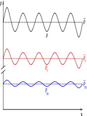
The most studied possibility is pure adiabatic initial mode. Then there is no entropy perturbation at , , but the total energy density fluctuates or more precisely there is a spatial perturbation in the comoving curvature . In Fig. 1(b) I have an example, where the spatial fluctuations in matter and radiation energy density are in the same phase yielding to an initial fluctuation in the total energy density.
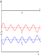
In the isocurvature case the specific entropy fluctuates spatially , but there is no initial fluctuations in the total energy density or more precisely in the comoving curvature, . For example, the fluctuation in matter and radiation could cancel each other giving spatially constant total energy density as in Fig 1(c).
The evolution of perturbations is described by second order differential equations, adiabatic and isocurvature initial conditions being two independent modes. Hence the most general initial condition is a mixture of adiabatic and isocurvature fluctuations. The evolution equations tell how adiabatic and isocurvature initial fluctuations are converted into the temperature fluctuation present at the last scattering surface and finally into the presently observable temperature (or polarization) anisotropy described by the angular power spectrum that contains a series of peaks and valleys. If the other cosmological parameters are kept fixed, but one changes form adiabatic initial conditions to the isocurvature ones, then the resulting angular power spectra are roughly in the opposite phases as can be seen in Fig. 2(a).
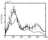
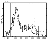
Already the first data sets by Boomerang and Maxima could be used to constrain uncorrelated mixture of adiabatic and isocurvature fluctuations in flat universe models. We found the maximum allowed isocurvature contribution to the quadrupole () temperature anisotropy to be 56% and to the first acoustic peak () about 13% , see Fig. 2(b). Since in open universe all the features of the angular power spectrum are shifted towards right (larger , smaller scales) and in closed universe towards left, it still seemed to be possible to fit the first acoustic peak by open or closed pure isocurvature models. However, the second data releases by Boomerang and Maxima identified also the second acoustic peak so well that the “adiabatic peak structure” became evident and we could finally rule out all pure CDM isocurvature models . From Fig. 2(c) one can see even by an eye that the pure isocurvature does very badly with the data. Nevertheless, mixed correlated or uncorrelated models remain as an interesting possibility.
2 Correlation and the WMAP
The initial fluctuations for the CMB physicist are the comoving curvature perturbation and the entropy perturbation at the beginning of the radiation dominated era. By hats I remind you that these are Gaussian random variables. They are related to the fluctuations at the horizon exit () during inflation by
| (1) |
where and are the transfer functions that describe the evolution of perturbations form to . In most cases, they are found only numerically by solving the evolution equations and modeling the reheating process.
The initial perturbations and are usually approximated by power laws ,
| (2) |
which is a good approximation assuming that “everything” changes slowly during inflation. Actually, e.g., in some cases of double inflation this is not true . In an ordinary pure adiabatic case one would have only the first term . Now I have additional terms coming from the entropy perturbation during inflation. In my terminology is called the first adiabatic component, the second adiabatic component (generated by the entropy perturbation during inflation if the trajectory in the multi field space is curved ), and the isocurvature component. , , and are amplitudes and spectral indices. Moreover, and are Gaussian random variables obeying , , and .
(a)
 (b)
(b)
 (c)
(c)
Now there is a 100 % correlation between the second abiabatic and the isocurvature component, . This can be parametrized by some overall amplitude (at the reference scale ) , isocurvature fraction , and correlation amplitude as follows: . The final angular power spectrum will be a combination of four different components: the first adiabatic, the second adiabatic, the isocurvature and the correlation between the second adiabatic and the isocurvature component
| (3) |
Wmap team already analyzed this kind of models , but for simplicity, they assumed the two adiabatic spectral indices to be equal, . This is not theoretically well motivated, since comes from the curvature perturbation and from the entropy perturbation. If one really needs to simplify the analysis, one should consider to put and equal.
In our Letter we allow for , , and to vary independently. To match the historical notation we redefine the spectral indices so that the value 1 corresponds to the scale free case: , , and . We use a grid method to scan the parameter space of 9 parameters ( combinations): , , , , , , , , and . Marginalization by integration is adopted, since some likelihoods are non-Gaussian.
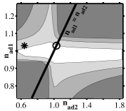
Fig. 3(a) shows our main result that the data do allow unequal adiabatic spectral indices, and actually, favour models where the two adiabatic components have opposite spectral tilts ( and or vice versa). This leads to a running effective adiabatic spectral index. The adiabatic initial power is , see equation (2) and the definitions above equation (3). Writing this as a single power law where is an amplitude and , one always gets non-negative first derivative for the common adiabatic spectral index ;
| (4) |
Using the wmap data only we get a upper bound for the isocurvature fraction, . Since the angular power alone cannot give “any” upper bound for the isocurvature spectral index, we have to put some prior for it; . We assume from the wmap team analysis that the large scale structure data (e.g., 2dF) would give about motivating our prior. In any case, we can compare our result to the result which we would get with the wmap team restriction . This simplification leads to unrealistically strict upper bound, .
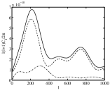
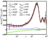
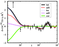
In Figs. 3(b)&(c) I have an example of a allowed correlated model. In the case of negative correlation, as here, the isocurvature contribution to the lowest multipoles in TT spectrum can be quite large due to cancellation by the correlation part. In TE spectrum the cancellation is not as exact so that there one gets enough power at the lowest multipoles. Actually, in this example, the isocurvature component dominates TE spectrum at the quadrupole . That is why even quite a small optical depth due to reionization () is enough to give a reasonable total power at the quadrupole. Thus in correlated models the measured high quadrupole in TE spectrum can be achieved without having as large as reported by the wmap team. So one should keep in mind a possible degeneration between the optical depth and correlation contribution. On the other hand, a positive correlation could nicely lead to even more power in TE at low , but unfortunately it tends to give a high quadrupole also in TT, which is not favoured by the data. An interesting possibility to explain the low quadrupole in TT would be to have a very strong negative correlation which “eats” some power from TT quadrupole. Then in TE this could be compensated by a large . Suitably strong negative correlation contribution to the total TT power requires that the second adiabatic and isocurvature components dominate over the first adiabatic component.
(a)
 (b)
(b)
 (c)
(c)
References
References
- [1] J. Valiviita and V. Muhonen, Phys. Rev. Lett. 91, 131302 (2003) [astro-ph/0304175].
- [2] H. V. Peiris et al., Astrophys. J. Suppl. 148, 213 (2003) [astro-ph/0302225].
- [3] C. L. Bennett et al., Astrophys. J. Suppl. 148, 1 (2003) [astro-ph/0302207].
- [4] A. Kogut et al., Astrophys. J. Suppl. 148, 161 (2003) [astro-ph/0302213].
- [5] “Code for Anisotropies in the Microwave Background”, http://camb.info/
- [6] K. Enqvist, H. Kurki-Suonio and J. Valiviita, Phys. Rev. D 62, 103003 (2000) [astro-ph/0006429].
- [7] C. B. Netterfield et al., Astrophys. J. 571, 604 (2002) [astro-ph/0104460]; A. T. Lee et al., Astrophys. J. 561, L1 (2001) [astro-ph/0104459].
- [8] K. Enqvist, H. Kurki-Suonio and J. Valiviita, Phys. Rev. D 65, 043002 (2002) [astro-ph/0108422].
- [9] C. Gordon, D. Wands, B. A. Bassett and R. Maartens, Phys. Rev. D 63, 023506 (2001) [astro-ph/0009131]; L. Amendola, C. Gordon, D. Wands and M. Sasaki, Phys. Rev. Lett. 88, 211302 (2002) [astro-ph/0107089].
- [10] C. Gordon, astro-ph/0112523.
- [11] S. Tsujikawa, D. Parkinson and B. A. Bassett, Phys. Rev. D 67, 083516 (2003) [astro-ph/0210322].