The Canada–France Deep Fields III: Photometric Redshift Distribution to $I_{\mbox{\small{AB}}}=24$

Abstract

We compute accurate redshift distributions to $I_{\mbox{\small{AB}}}=24$ and $R_{\mbox{\small{AB}}}=24.5$ using photometric redshifts estimated from six–band $U\!BV\!RI\!Z$ photometry in the Canada–France Deep Fields–Photometric Redshift Survey (CFDF–PRS). Our photometric redshift algorithm is calibrated using hundreds of CFRS spectroscopic redshifts in the same fields. The dispersion in redshift is $\sigma/(1+z)\lesssim 0.04$ to the CFRS depth of $I_{\mbox{\small{AB}}}=22.5$, rising to $\sigma/(1+z)\lesssim 0.06$ at our nominal magnitude and redshift limits of $I_{\mbox{\small{AB}}}=24$ and $z\leq 1.3$, respectively. We describe a new method to compute $N(z)$ that incorporates the full redshift likelihood functions in a Bayesian iterative analysis and we demonstrate in extensive Monte Carlo simulations that it is superior to distributions calculated using simple maximum likelihood redshifts. The field–to–field differences in the redshift distributions, while not unexpected theoretically, are substantial even on 30′ scales. We provide $I_{\mbox{\small{AB}}}$ and $R_{\mbox{\small{AB}}}$ redshift distributions, median redshifts, and parametrized fits of our results in various magnitude ranges, accounting for both random and systematic errors in the analysis.

1. Introduction

The last decade has seen great advances in our understanding of the evolution of the Universe, primarily due to groundbreaking studies of the intermediate (Lilly et al., 1995b) and high redshift (Steidel et al., 1996) Universe. These ”pencil beam” surveys probed to cosmological depths over quite modest areas, revealing the strong luminosity, morphological, and clustering evolution of the galaxy population over the last 12 Gyr. It was, however, recognized at the time that the small windows on the Universe provided by these surveys were subject to substantial sample, or “cosmic” variance, in particular for measurements on the scale of the survey field sizes.

Recently the 2dF (Colless et al., 2001) and SDSS (York et al., 2000) surveys provided the first precise ”local” ($z\sim 0.1$) measurements of the galaxy luminosity function (Norberg et al. 2002b; Blanton et al. 2003), providing a crucial baseline reference for evolutionary studies. In addition, measurements of the galaxy correlation function in these surveys (Norberg et al., 2002a; Zehavi et al., 2002) have convincingly demonstrated luminosity–dependent clustering long seen at lower significance in smaller samples. These surveys finally overcame the cosmic variance issues that had plagued previous local surveys by sampling over 10³ square degrees.

With the advent of large format mosaic CCDs, we undertook the Canada–France Deep Fields (CFDF) survey, a deep $U\!BV\!I$ imaging survey in four $30\arcmin\times 30\arcmin$ fields. Published results from the CFDF include a study of the galaxy angular correlation function to $I_{\mbox{\small{AB}}}=25$ (McCracken et al., 2001), and a measurement of the clustering properties of Lyman–break galaxies at $z\sim 3$ (Foucaud et al., 2003). In this paper we introduce the CFDF Photometric Redshift Survey (CFDF–PRS), derived from a highly uniform $U\!BV\!RI\!Z$ sub–sample of the main survey, which forms the basis of several evolutionary measurements of the galaxy population as a function of redshift. Future papers (Brodwin et al, in preparation) will present studies of the galaxy luminosity and correlation functions.

In this paper we focus on an accurate measurement of the galaxy redshift distribution from $0<z<1.3$. We introduce a novel iterative technique to extract the optimal redshift distribution using the full redshift likelihood functions for each galaxy. We present binned redshift distributions along with parametrized fits to our results.

The outline of this paper is as follows. Section §2 briefly describes the CFDF–PRS data. Section §3 describes the calculation and calibration of the photometric redshifts. Section §4 introduces the iterative Bayesian method of recovering the redshift distribution using the full redshift probability function for each galaxy. In Sections §5 and §6 we present the photometric redshift distributions, obtained using the iterative method, as a function of sample limiting magnitude in the CFDF down to $I_{\mbox{\small{AB}}}=24$ and $R_{\mbox{\small{AB}}}=24.5$, both in half magnitude bins and via parametrized fits. Finally, in Section §7 we summarize our results.

Most of our results are independent of cosmology. Where necessary we have assumed a concordance cosmology in agreement with the recent WMAP (Spergel et al., 2003) results $\{\Omega_{M},\Omega_{\Lambda}\}=\{0.27,0.73\}$ and a Hubble constant $h=0.71$ where $H_{0}=100\,h$. All distances are expressed in comoving Mpc.

2. Canada–France Deep Fields

The Canada–France Deep Fields (CFDF) is a deep, multi–color imaging survey covering 1 deg² (McCracken et al. 2001; Foucaud et al. 2003, hereafter CFDF1 and CFDF2, respectively). The acquisition, reduction, and verification of the astrometric and photometric integrity of the original $U\!BV\!I$ data are described extensively in CFDF1. This first paper in the series also includes extensive completeness simulations showing that the survey is $\sim 90\%$ complete to $I_{\mbox{\small{AB}}}\leq 24$. Deep $B_{\mbox{\small{AB}}}$ and $I_{\mbox{\small{AB}}}$ galaxy counts along with a detailed angular clustering analysis confirm the reliability of the data to at least this depth.

2.1. Supplementary $\mathbf{R}$ and $\mathbf{Z}$ Imaging

Photometric redshift simulations described elsewhere (Brodwin et al., 1999) indicated the need for additional $R$– and $Z$–band imaging to produce accurate photometric redshifts out to $z\sim 1.3$. Further deep CFHT imaging was obtained in these bands, along with some additional $I$ and $B$ imaging to replace time originally lost to bad weather. We replaced the UH8k data with this superior, deeper CFH12k $I$ and $B$ data, since combining the two datasets would have degraded the excellent CFH12k seeing and cosmetic quality and while adding little in terms of depth. These data were reduced, stacked and calibrated using standard procedures (e.g. bias subtraction, flat fielding, fringe removal, geometric distortion correction), carefully adapted to mosaic CCD imaging as described in CFDF1 and Brodwin (2004).

New catalogues for this work were generated using the $\chi^{2}$ technique of Szalay et al. (1999). The various magnitude limited galaxy samples studied in this paper were selected using total magnitudes as measured by the Sextractor (Bertin and Arnouts, 1996) MAG_AUTO parameter, whereas the photometric redshifts are computed using 2.5″ diameter aperture magnitudes.

Star/galaxy classification was performed using a hybrid technique that incorporates both morphology (in 0.6″$Z$–band images) and 4 color-color planes of information (see Brodwin 2004 for full details). Only objects extremely reliably classified as stars are removed from the present analysis.

2.2. Photometric Redshift Sample

As explained in CFDF2, $U$–band imaging only exists in 2.5 of our 4 $30\arcmin\times 30\arcmin$ fields. In addition, data in one of the eight UH8k CCDs with which the original data was taken is not science grade, due to bad charge transfer efficiency. Limiting the survey to those regions containing 6–band photometry, and excluding the regions masked due to bright (and saturated) stars, scattered light, remnant cosmetic defects that survived the median stacking, and the aforementioned unreliable CCD, resulted in a final CFDF–Photometric Redshift Survey (CFDF–PRS) area of 0.45 deg². Although such conservative cuts remove over half of the original survey area from the PRS, the remaining data is of very high quality and uniformity, and has the wavelength coverage necessary for robust photometric redshifts. The final photometric sensitivities for the CFDF–PRS are presented in Table 1.

Table 1Final Photometric Sensitivities in the CFDF–PRS.

Field	R.A.	Dec.	Area	Band	5$\sigma$/2.5″	Seeing
	(2000)	(2000)	(deg2)		(AB mags)	(arcsec)
03hr	03:03:00	+00:09:00	0.17	U	25.17	1.0
				B	25.41	0.80
				V	25.04	1.3
				R	25.15	0.95
				I	25.04	0.70
				Z	24.26	0.65
14hr	14:17:10	+52:24:43	0.18	U	25.88	1.4
				B	25.33	0.80
				V	25.04	1.0
				R	25.21	0.95
				I	24.51	0.70
				Z	24.47	0.70
22hr	22:17:48	+00:17:13	0.10	U	25.96	1.4
				B	25.23	0.8
				V	25.18	1.0
				R	25.42	0.90
				I	25.36	0.75
				Z	24.65	0.52

3. Photometric Redshift Algorithm in the CFDF–PRS

In order to estimate photometric redshifts and calculate the redshift probability distributions needed for the present study as well as the luminosity and clustering analyses of future CFDF papers (Brodwin et al. in preparation), we employ a standard empirical template fitting algorithm, in which filter-convolved empirical galaxy template SEDs are fitted to the observed galaxy photometry to determine the best–fitting redshift and spectral type. To obtain robust galaxy colors the photometry in each filter is co–convolved to the worst seeing in each field (1.3″-1.4″). The photometry is fitted to the templates in the flux domain, with the flux error for each object taken as the quadrature sum of its Poisson noise and a Monte Carlo estimate of the sky error in the aperture.

The Coleman et al. (1980, hereafter CWW) empirical SEDs, supplemented by the Kinney et al. (1996) SB2 and SB3 starburst SEDs, were adopted as the basis templates. This combination of templates has been shown to span the range of galaxy properties in the HDF from $0<z<6$ (Benítez, 2000; Fernández-Soto et al., 1999). The CWW templates were extended into the far UV using normalized solar metallicity GISSEL models. The Kinney et al. (1996) starburst SEDs, well measured down to $\sim 1100$ Å, were extended to 912 Å via simple linear extrapolation. Fifteen interpolates of these basis spectra were used to improve the redshift resolution. Galaxy reddening is naturally incorporated into our empirical templates, as they are each composite spectra from numerous galaxies with varying levels of extinction. Our SEDs are statistically corrected for intergalactic hydrogen absorption as a function of redshift following Madau (1995), taking into account both Lyman series line blanketing at wavelengths below $\lambda_{\mbox{\scriptsize obs}}<1216\,(1+z)$ Å and continuum photoelectric absorption below the Lyman limit, $\lambda_{\mbox{\scriptsize obs}}<912\,(1+z)$ Å. A maximum likelihood method (ML) was used to produce the redshift likelihood surface for each object as a function of redshift and spectral type.

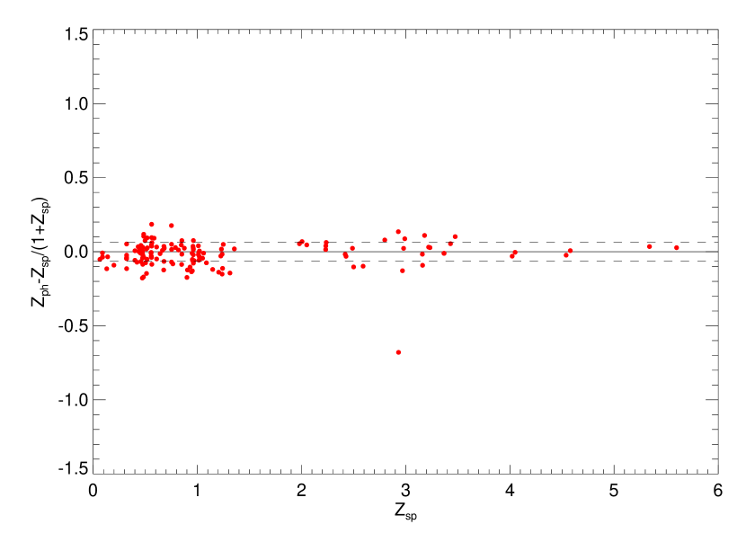
This code was tested extensively with public HDF data and using the hundreds of CFRS spectroscopic redshifts in our fields. The latter sample allowed a novel form of calibration of the method, described below, to significantly improve the redshift accuracy. In the HDF, the simple ML redshifts matched the excellent results in the literature (Fernandez-Soto et al., 2002; Benítez, 2000; Fontana et al., 2000; Sawicki et al., 1997; Connolly et al., 1997), as shown in Figure 1, with redshift dispersions of $\sigma_{z}\sim 0.07\,(1+z)$ over the full redshift range $0<z<6$ and only one “catastrophic error” (for a discussion of this object see Fernandez-Soto et al., 2002). The photometric redshifts described in this Section have not been subjected to a Bayesian prior. In Section 4 we demonstrate how the use of such a prior improves the derived redshift distribution.

Figure 1.— Photometric redshift residuals for spectroscopic galaxies in the HDF North for the sample defined in Fernandez-Soto et al. (2002). This Figure is directly comparable to their Figure 7. The dashed lines enclose the 1$\sigma$ error interval, which, excluding the single discrepant galaxy, is $\Delta z/(1+z)=0.07$.

3.1. Calibration Using CFRS Spectroscopic Redshifts

The accuracy of photometric redshift estimation can be improved using a spectroscopic training set (see, e.g., Csabai et al., 2003). Taking the CFRS galaxies with the most secure spectroscopic redshifts (confidence class 3 and 4, see Le Fèvre et al. 1995 for details), we have a training set of 321 galaxies between $0\leq z\leq 1$ and $18.5\leq I_{\mbox{\small{AB}}}\leq 22.5$ (where the bright limit is imposed by the saturation limit of the CFDF–PRS). We use this spectroscopic sample as a novel kind of calibrator to improve the photometric calibration in our three fields, thereby producing significantly more accurate redshift estimation.

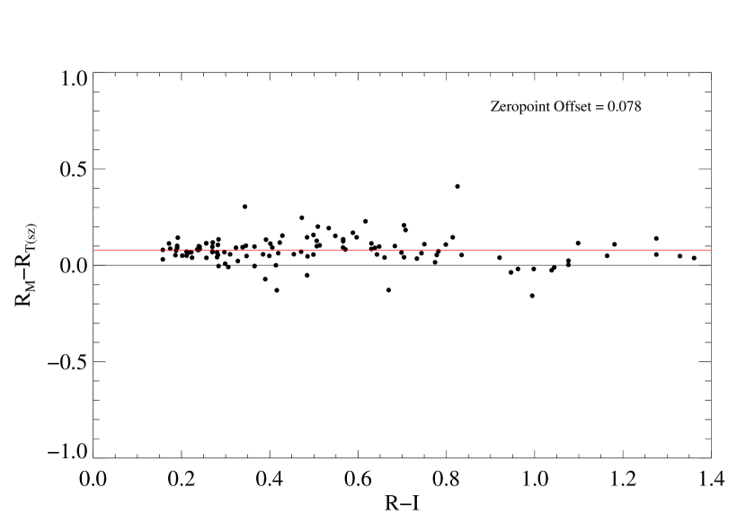
We examined the residuals between the observed magnitude and the best–fitting template at the correct (spectroscopic) redshift in each band, as a function of the color of the galaxies. As an example, if all galaxies, regardless of redshift or spectral type, showed a residual, $\Delta m$, in some band, that would suggest that there was a zero point offset of $\Delta m$ in that filter. If $\Delta m$ was correlated with the color of the objects, that could indicate an error in the filter effective wavelength (the origin of which is inaccurate filter transmission or QE curves), or problems with the template SEDs. In practice such color terms were negligible as expected, whereas small but significant zeropoint offsets were found in several filters. These offsets are caused, in part, by band–to–band seeing variations not fully removed when we convolve our images in each filter to the same seeing. Such residual seeing variations would manifest as zeropoint offsets. Almost all calculated offsets were less than 0.1 mag, the largest being 0.12 mag. An example is shown in Figure 2 for the $R$ filter in the 03hr field.

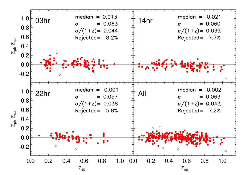
This optimal calibration produces photometric redshifts with comparable error properties in all three CFDF–PRS fields, as shown in Figure 3. The redshift dispersion, in the common measure in which the error increases as $(1+z)$ is $\sigma_{z}/(1+z)=0.042$ for galaxies within the iteratively clipped $3\,\sigma$ limits of the distribution (solid circles). The direct dispersion for this sample, which includes over $92\%$ of the galaxies is $\sigma_{z}=0.062$.

Figure 2.— Residuals between the measured $R$ magnitudes and the best–fitting template SEDs redshifted to the spectroscopic redshifts versus galaxy color. This technique essentially identifies the optimal photometric zero point and the effective wavelength in each broadband filter, using the CFRS galaxies as photometric standards. In this 03hr $R$ band plot, the zeropoint offset is $\sim 0.08$ magnitudes.

Figure 3.— Residuals in photometric vs. spectroscopic redshift for the CFRS spectroscopic galaxies in each field and for the full survey. For almost $93\%$ of $I_{\mbox{\tiny{AB}}}\leq 22.5$ CFRS galaxies that fall within the iteratively clipped 3$\sigma$ limits of the distribution (solid circles) the redshift dispersion is $\sigma\sim 0.06$. In the commonly used $\sigma/(1+z)$ measure the dispersion for this sample drops to $\sim 0.04$. Objects represented by open circles were rejected as outliers for calculation of the dispersion.

It is important to stress that no bias was introduced to the CFDF–PRS through the use of the CFRS spectroscopy. The true redshifts were used to transform the CFRS galaxies present in the CFDF–PRS into photometric standards, which were in turn used to tweak our zeropoints. Given the spectroscopic redshifts, the process is completely internal to the CFDF–PRS photometry, and results in optimal photometric redshifts for our depth and wavelength coverage.

3.2. Photometric Redshift Accuracy for $I_{\mbox{\small{AB}}}>22.5$ Galaxies

In order to test the accuracy of photometric redshifts at magnitudes fainter than the CFRS data, we added a scaled version of each image in each field back to itself, with a positional offset larger than the full CFRS field. Care was taken to ensure that the noise properties of the resulting images were identical to those of the original images. Specifically, in each field and filter we multiplied the original image by a scale factor, $f_{1}$, translated this scaled image by $\sim 10\arcmin$, and added it back to the original image. We then divided this new image by $(1+f_{1}^{2})^{0.5}$ to restore the original image’s noise properties. The scale factor, $f_{1}$, is chosen such that in the final image CFRS galaxies with $I_{\mbox{\small{AB}}}=22.5$ are transformed into $I_{\mbox{\small{AB}}}=24$ objects (i.e. a 1.5 magnitude change $\rightarrow f_{1}\approx 0.2595$).

These fainter CFRS galaxies were photometered, and photometric redshifts were computed as above. The results, shown in Figure 4, demonstrate that while the increasing photometric error only modestly affects the redshift dispersion in each field to $I_{\mbox{\small{AB}}}\sim 24$, the fraction of outliers in our 3$\sigma$ clipping algorithm increases to as much as $\sim 15\%$. Clearly just using the maximum likelihood values of the redshift is problematic in statistical analyses of these faint galaxies.

While this exercise demonstrates the effect of increased photometric errors on redshift estimation, it implicitly assumes that $I_{\mbox{\small{AB}}}<24$ galaxies are basically just fainter copies of CFRS galaxies. It does not address the possibility that at this fainter flux limit a new, distinct galaxy population may emerge, one which may be intrinsically unlike our empirical galaxy templates. Photometric redshift accuracy for such galaxies would likely be quite poor, and the paper’s main results could be substantially compromised. However, no evidence for such a hypothetical population is seen in the public HDF, where the spectroscopic sample extends to $I_{\mbox{\small{AB}}}\sim 25$ and beyond. Indeed the excellent photometric redshift accuracy achieved by our code in this sample indicates that the CWW and Kinney et al. (1996) templates provide a good description of galaxies to very faint magnitudes over $0<z<6$. We conclude that the effect on our primary results by any fundamentally different galaxy population which may emerge between $22.5<I_{\mbox{\small{AB}}}<24$ is minimal.

Figure 4.— Residuals in photometric vs. spectroscopic redshift for galaxies to $I_{\mbox{\tiny{AB}}}\leq 24.0$. The difference in imaging depths between the three CFDF–PRS fields is becoming apparent. In the 22hr field, the redshift dispersion and number of outliers is largely unchanged from the brighter sample in Figure 3. In contrast, the number of outliers in our 3$\sigma$ clipping algorithm has doubled to 17% in the 14hr field. The redshift dispersions, in each field and overall, are still less than $\sigma\sim 0.1$ to $I_{\mbox{\tiny{AB}}}\sim 24.0$.

3.3. Photometric Redshift Accuracy for $z\sim 3$ Lyman Break Galaxies

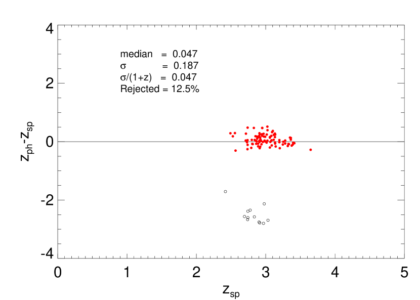
To test the photometric redshift algorithm at redshifts much higher than the CFRS, we have used the Steidel et al. (2003) spectroscopic sample of $z\sim 3$ Lyman Break galaxies (LBGs) present in our 14hr field (the “Groth strip”). We photometer the LBG positions in this field and compute redshifts for objects with S/N $\geq 3$. Figure 5 shows the redshift residuals for the $104$ spectroscopic LBGs above this limit. This sample, being extremely limited in redshift space, is instructive in exploring the occurrence of catastrophic redshift errors. The filled symbols are well measured redshifts, whereas the open symbols, representing $\sim 13\%$ of the sample, are catastrophic failures. Neglecting these the photometric redshifts at $z\sim 3$ have a dispersion of $\sigma/(1+z)\sim 0.05$.

The catastrophic failures in this LBG sample stem from the difference in the $U$ filters between the two surveys. The Steidel et al. (1996) bluer $U_{n}$ filter allows selection of robust LBG candidates at slightly lower redshifts than our $U$ filter (in which the Lyman continuum break is only centered at $z\sim 3.2$). The extremely faint $z\sim 2.8$ Steidel et al. (2003) LBGs, without a strong continuum break fully bracketed by our filters, suffer a degeneracy between the $z\sim 2.8$ starburst and $0\lesssim z\lesssim 0.5$ redder galaxy types. Approximately $20\%$ of the faint $2.7\leq z\leq 3.0$ LBGs are misclassified as lower redshift galaxies.

It is important to note that in this work, in addition to only using objects with S/N $\geq 10$, we are restricting ourselves to a redshift range which always contains the 4000 Å break.

Figure 5.— Residuals in photometric vs. spectroscopic redshift for $104$ Steidel et al. (2003) Lyman Break galaxies with S/N $\geq 3$ in the CFDF–PRS 14hr field. Excluding catastrophic errors (open symbols), the dispersion in redshift is $\sigma/(1+z)\sim 0.05$. The galaxies with catastrophic errors, roughly $\sim 13\%$ of the sample, are clustered below $z\sim 3$ where our filters do not fully straddle a strong continuum break.

3.4. Statistical Validity of Redshift Likelihood Functions: Confidence Intervals

In Section §4 we introduce a new method of calculating $N(z)$ in photometric redshift surveys using the full redshift likelihood function for each galaxy. Here the error properties of the likelihood functions are characterized using the CFRS spectroscopic sample. Following Fernández-Soto et al. (1999) we define the 1, 2, and 3–$\sigma$ confidence intervals as those redshift regions which enclose the top 68.3%, 95.4%, and 99.7% of the area in our normalized redshift likelihood functions. At this point the likelihood functions have not been subjected to any prior (i.e there is equal a priori likelihood at all redshifts).

We found that convolving the likelihood functions with a Gaussian with $\sigma=0.04$ produced approximately normal confidence level statistics, as shown in Table 2, and has the beneficial effect of smoothing the likelihood functions. We note that the smoothing kernel is less than our redshift dispersion of $\sim 0.06$ measured with the CFRS spectroscopic sample. Examples of representative likelihood functions for $I_{\mbox{\small{AB}}}=[21,~{}22,~{}23,~{}24]$ galaxies are shown in Figure 6.

Figure 6.— Typical likelihood functions with 1$\sigma$, 2$\sigma$, and 3$\sigma$ confidence intervals for increasingly fainter galaxies. At the survey limit the likelihood functions become multiply–peaked, leading to disjoint, but nevertheless statistically valid confidence intervals.

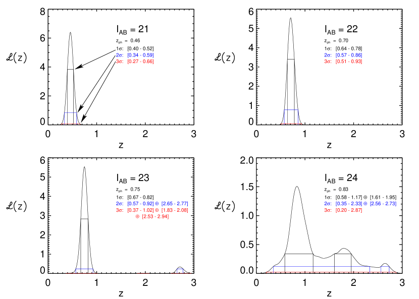
Brighter than $I_{\mbox{\small{AB}}}\lesssim 23.5$ the likelihood functions are overwhelmingly single–peaked, approximately Gaussian probability distributions, with relatively little probability density in secondary peaks. At the survey limit, however, the secondary peaks become increasingly significant, often leading to multi–moded, disjoint confidence intervals even at the 1$\sigma$ level.

Table 2Statistics of confidence intervals derived from redshift likelihood functions for CFRS spectroscopic galaxies.

Confidence	Observed	Expected
Interval	Number	Number
$\leq 1\sigma$	235/321	219  ${}^{+16}_{-15}$
$\leq 2\sigma$	306/321	306  ${}^{+19}_{-18}$
$\leq 3\sigma$	315/321	320  ${}^{+19}_{-18}$
$>3\sigma$	6/321	000.9  ${}^{+2.2}_{-0.8}$

The confidence level statistics are nevertheless quite consistent with a normal error distribution in the Poissonian limit, as shown in Table 2, although we place a slightly higher fraction of galaxies beyond the 3–$\sigma$ error limit. The Poisson errors on the expected number of galaxies are computed using the Gehrels (1986) expressions valid for small numbers of events. This exercise verifies the statistical validity of our redshift likelihood functions and of the analysis presented in Section §5 that incorporates them.

4. Method: Constructing Photometric Redshift Distributions

For high S/N photometry like that in the HDF, where the redshift likelihood functions are overwhelmingly narrow and singly–peaked, it is sensible to simply adopt the redshift which maximizes the likelihood as the photometric redshift. However, an open question is how to best measure photometric redshift distributions in the lower signal–to–noise photometry typical of ground–based surveys. The present method addresses this issue in the CFDF–PRS and in anticipation of upcoming wide–field near–HDF depth imaging surveys (such as the CFHT Legacy Survey).

Detailed Monte Carlo simulations (described below) demonstrate that simple maximum likelihood photometric redshift methods increasingly fail to reproduce the underlying redshift distribution at S/N $\lesssim 20$. This Section describes a Bayesian method for recovering the underlying $N(z)$ at still more modest S/N levels using the ensemble redshift information present in the data.

4.1. Bayesian Photometric Redshift Distributions

As described in detail in Benítez (2000), Bayesian statistics provide a way to incorporate our knowledge about the galaxy distribution to improve the photometric redshift accuracy. This is accomplished through the use of priors on the simple likelihood functions, which by nature assume all redshifts are a priori equally likely. The prior converts the likelihood functions into true Bayesian redshift probability distributions which can be incorporated directly into cosmological studies in place of traditional spectroscopic redshifts (which, in general, can be thought of as approximately $\delta$–function redshift probabilities).

Specifically,

$$P(z,T)\propto P[z,T|\,N(z)\,]\times{\cal L}(z,T)$$ (1)

where ${\cal L}(z,T)$ is the likelihood of measuring the observed colors for a galaxy of spectral type T at redshift z. In the Bayesian interpretation $P[z,T|\,N(z)\,]$ is a prior, in this case the probability of drawing a galaxy with redshift z and type T from a redshift distribution $N(z)$. This prior, applied to the likelihood function, incorporates the basic fact that all redshifts are not a priori equally likely. As the goal here is to measure a statistical property of the galaxy population, namely its redshift distribution, requiring this information a priori may appear somewhat circular. However, we have devised an iterative scheme to recover the underlying redshift distribution and tested it in detailed Monte Carlo simulations.

4.2. Direct summation of $N(z)$ and Iteration

Rather than adopting the simple maximum likelihood (ML) value of each galaxy redshift, we choose instead to directly sum up the normalized likelihood functions, ${\cal L}^{n}$, of each galaxy in the photometric sample. This would trivially produce the correct redshift distribution in the limit of spectroscopic (i.e. $\delta$–function) input redshifts. For photometric redshifts in the high signal–to–noise regime this method yields approximately the same result as collapsing the ${\cal L}^{n}$ to the single maximum likelihood redshift since the ${\cal L}^{n}$ are typically single sharp Gaussians. At fainter magnitude limits, the likelihood functions become broader and often develop multiple peaks as degeneracies between distinct templates at different redshifts arise with the increasing photometric error. With simple ML redshifts the derived $N(z)$ is both too broad and has artificial peaks as significant numbers of galaxies are shifted between these degenerate redshifts. This is true as well of the first step of our iterative method:

$$N^{0}(z)=\sum_{i}{\cal L}_{i}^{n}(z)=\sum_{i}\frac{{\cal L}_{i}(z)}{\int_{0}^{\infty}{\cal L}_{i}(z)\,dz}.$$ (2)

This zeroth order redshift distribution, $N^{0}(z)$, is then used as the prior, $P[z,T|\,N(z)\,]$, in an iterative solution to equation 1. This prior uses the bulk information present in the galaxy colors to modify the raw likelihoods so as to minimize the degeneracies and, in effect, deconvolve the individual likelihood functions of the low S/N broadening effect. The resulting distribution serves as the first order prior, $N^{1}(z)$, and the procedure can be carried on to convergence, which, as shown in the following Section, is so rapid that additional steps are unnecessary.

This method makes the assumption that a single prior is applicable to galaxies of all brightnesses and spectral types in a given sample. Ideally, each population of galaxies should have its own unique prior to optimally weight the simple likelihood functions. Although the use of a single statistical prior, in this case the iteratively estimated redshift distribution, is obviously a rough approximation, we demonstrate that it works surprisingly well. This should not be mistaken to imply that redshifts of individual galaxies are uniformly improved with this method. It is the complete statistical redshift distribution that is demonstrably improved compared with that obtained via the standard method of collapsing the redshift likelihood function of each galaxy to a single maximum likelihood redshift.

Obviously the method breaks down at very low signal–to–noise. Extensive testing of the convergence properties of the method, presented in Brodwin (2004) and summarized in the Appendix, indicates that the convergence is excellent over the range $0.2\leq z\leq 1.3$ for S/N $\gtrsim 10$. This is confirmed in the simulations described in the next Section.

4.3. Test of the Method: Monte Carlo Simulation

The iterative method described above was extensively tested in detailed Monte Carlo simulations. Briefly, model Universes were populated according to CNOC2 evolving luminosity functions (Lin et al., 1999) for early, intermediate and late spectral types, modified to produce a range of reasonable input redshift distributions to $z>3$. These model galaxies were assigned colors using the empirical template set used in the CFDF photometric redshift code, ranging from the CWW Elliptical (Coleman et al., 1980) to the Kinney et al. (1996) SB2. Flux errors matching the $U\!BV\!RI\!Z$ photometry in the CFDF fields were applied to these galaxies, and photometric redshift likelihood functions were computed for galaxies in an area of 0.5 deg². A systematic error not accounted for in this simulation is the possible incompleteness of the adopted template SEDs with respect to the true range of galaxy properties. This was approximately accounted for following the method of Fernández-Soto et al. (1999) by convolving the computed redshift likelihood functions with a variable–width Gaussian,

$${\cal L}^{c}(z)=\int_{0}^{\infty}dz^{\prime}\,{\cal L}(z^{\prime})\,\,G\left[z|z^{\prime},\Sigma(1+z^{\prime})\right],$$ (3)

where G is a normalized Gaussian (truncated at $z<0$) of median z’ and $\sigma=\Sigma(1+z^{\prime})$. $\Sigma$ was set to 0.05 based on a detailed comparison with CFRS spectroscopic redshifts, as described in Section §3.1 (in fact, this is $\sim 20\%$ larger than was found for the CFRS, but was adopted in a conservative vein).

4.3.1 Simulation Results

In the interest of clarity we briefly recall the various methodologies this simulation was designed to test. The basic technique for computing redshift distributions consists of making a simple histogram of the best–fitting photometric redshifts for each galaxy. This is identical to taking the redshift that maximizes the likelihood function in likelihood-based fitting algorithms. We therefore dub this the Peak–ML method. Our new method, essentially a two–step iterative process, uses the full redshift likelihood function for each galaxy in computing $N(z)$. We therefore label it the Full–RLF iterative method (sometimes referred to simply as the RLF method for brevity). Redshift distributions were computed using both the Peak–ML method and the Full–RLF iterative method, and compared to the input $N(z)$. While the final iteration of the Full–RLF method is superior down to $I_{\mbox{\small{AB}}}\leq 24.0$, the improvement is most pronounced for the $I_{\mbox{\small{AB}}}\leq 23.5$ sample, which we plot in Figures 7 and 8.

Figure 7.— Results of Monte Carlo simulations testing Peak–ML (open circles), Initial RLF (dashed curve) and Final RLF (solid curve) methods for computing $N(z)$ in a photometric redshift survey. The filled circles show the input (model) $N(z)$. The Peak–ML and Final RLF methods both recover the underlying $N(z)$ quite faithfully, but the latter is in fact significantly better as discussed in the text and illustrated in Figure 8. Note how the aliased peak at $z\sim 1.9$ in the Initial RLF iteration is strongly suppressed in the Final RLF distribution, reproducing the model $N(z)$ better even than the Peak–ML method.

Figure 8.— Contribution to $\chi_{\nu}^{2}$ from each redshift bin for the Peak–ML (sparsely filled histogram), Initial RLF (empty histogram) and Final RLF (densely filled histogram) methods. Note the significant improvement over the Initial RLF method provided by both the Peak–ML and Final RLF distributions. The advantage of the Final RLF over the Peak–ML method is also apparent, as the differential $\chi_{\nu}^{2}$ of the former is lower in each bin, often dramatically. The total $\chi_{\nu}^{2}$ (i. e. summing over redshift) for these samples is {Initial RLF, Peak–ML, Final RLF} = {14.5, 4.02, 1.25}.

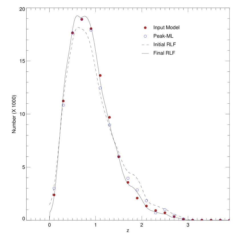
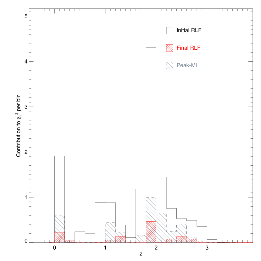
Figure 7 plots the redshift distributions obtained with the various methods. The filled and open circles represent the input (model) and Peak–ML redshift distributions, respectively. The dashed and solid lines show the Initial and Final iterations of the RLF method, respectively.

At first glance, all the methods appear to reproduce the input $N(z)$ quite well. However, upon closer examination, it is clear that the Initial RLF $N(z)$ is inferior to both the Peak–ML and the Final RLF distributions. On a qualitative level, we see that an incorrect secondary peak at $z\sim 1.9$ draws galaxies away from the main peak at $z\sim 0.7$. This problem is most acute for the Initial RLF method, but is nevertheless evident in the Peak–ML points. The Final RLF method appears to suffer less from the effect of this photometric redshift degeneracy.

In fact, the trends observed with the different methods can be easily understood. Objects with little redshift ambiguity (i.e. narrow, singly–peaked redshift likelihood functions) contribute to the different $N(z)$ measures in the same, correct way. On the other hand, those objects whose redshift likelihood functions show a strong degeneracy (i.e. at least two similar peaks at distinct, aliased redshifts) contribute to $N(z)$ in quite different ways in the above methods. In these cases the Peak–ML method usually selects the correct redshifts, although the catastrophic fraction increases with decreasing S/N. The main features of the input $N(z)$ are therefore fairly well reproduced, although small peaks from the catastrophic errors will arise at specific aliased redshifts. The Initial RLF method, as the direct sum of the likelihood functions, will always underpredict the main $N(z)$ peak as all the probability density of incorrect peaks at aliased redshifts is removed from it, leading to quite large peaks at the aliased redshifts. The Final RLF method, which uses the Initial RLF distribution as a prior, strongly suppresses these incorrect peaks using the information contained in the bulk of the galaxy sample (which is, on the whole, correct), bringing most of the ambiguous redshifts into line. A quantitative analysis demonstrates the superiority of the Final RLF method, and shows that it represents a significant improvement over the Peak–ML method.

To quantitatively assess the different methods we compare the resulting $N(z)$ of each method to the input $N(z)$ using a $\chi^{2}$ test. To make a fair comparison, we integrate the iterative method curves over each Peak–ML redshift bin to produce a binned version of the iterative method for this test. The Initial RLF redshift distribution has a reduced $\chi_{\nu}^{2}=14.5$ when compared with the input $N(z)$. The Peak–ML method, unsurprisingly, is much better, with $\chi_{\nu}^{2}=4.02$. It should be remembered that photometric redshift errors are not formally Gaussian. In fact in the low S/N regime, where multiple peaks arise, the error distribution is patently non–Gaussian, rendering impossible a direct confidence interval interpretation of the absolute $\chi^{2}$ values. However, regardless of the nature of the photometric error distribution, reductions in $\chi^{2}$ should indicate relatively better fits. In the Final RLF method the distribution no longer suffers from the effects of the redshift aliasing. The curve runs through (or very near) all the input $N(z)$ data points, and the $\chi_{\nu}^{2}$ drops to $1.25$.

Figure 8 shows the individual contribution from each redshift bin to the total value of $\chi_{\nu}^{2}$ for each method. The dramatic improvement from the Initial RLF (empty histogram) to Final RLF (densely filled histogram) is evident. The resulting $N(z)$ has smaller deviations from the input distribution in every bin compared with the Peak–ML redshift distribution (sparsely filled histogram).

It is interesting to note that in this simulation the iterative method accurately recovers the redshift distribution outside the “guaranteed–convergence” redshift range of $0.2\lesssim z\lesssim 1.3$ (see Appendix). Various input redshift distributions and binnings have been investigated, with results consistent with those shown in Figure 7.

In addition to the $\chi^{2}$ tests Kolmogorov–Smirnov (K–S) statistics were computed for all methods. The same pattern emerges, in which the Peak–ML method produces a redshift distribution more consistent with the input distribution than the Initial RLF method, but much less consistent than the Final RLF method. In this test the results are not impressive in either of the former two cases, with the somewhat better Peak–ML redshift distribution matching the input distribution at a probability of only $10^{-3}$. This is perhaps not surprising given the relatively high $\chi^{2}$ test result. On the other hand, the final iteration of the Full–RLF method has a K–S probability of $0.31$ of matching the input distribution, which is the level of variation expected in a Poisson sampling of the underlying distribution.

5. Redshift Distributions in the CFDF–PRS

The iterative method was applied to the CFDF–PRS data described in Section §2. At bright magnitudes our results can be compared directly with the CFRS redshift distributions (Crampton et al., 1995, hereafter CFRS5).

5.1. Comparison with the CFRS

The three CFDF–PRS fields contain 3 of the 5 small fields in which the CFRS survey was carried out. We can therefore compare the redshift distributions of each field individually, as well as the aggregate results for the two surveys to the CFRS limit of $I_{\mbox{\small{AB}}}=22.5$. It is important to stress that these surveys are completely independent. The imaging data was taken with different cameras and filters, and the photometric calibrations are entirely independent. The CFRS magnitudes are isophotal, whereas in the CFDF we use SExtractor (Bertin and Arnouts, 1996) total magnitudes (MAG_AUTO).

Figure 9 compares the $18.5\leq I_{\mbox{\small{AB}}}\leq 22.5$ redshift distributions in each common field as well as for the sum of the fields. The solid curve is the Final RLF redshift distribution, the open circles represent the Peak–ML method, and the histogram is the original CFRS redshift distribution.

Figure 9.— CFDF–PRS and CFRS redshift distributions over the common magnitude range $18.5\leq I_{\mbox{\tiny{AB}}}\leq 22.5$. The curves are the Full–RLF final iteration, the open circles represent the Peak–ML distributions, and the histograms are from the CFRS. In the individual fields the CFRS number densities are scaled to the CFDF values, whereas in the combined fields we plot the CFRS distribution using their original normalization. The fraction of unidentified CFRS objects is represented by the box to the left of the peak. Stars have been removed from both samples.

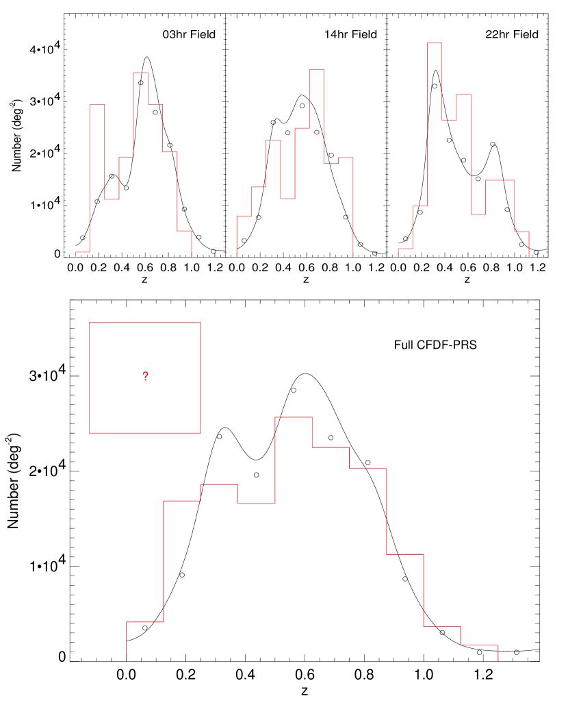
The agreement in all three fields is remarkable, though not at all tautological. To this depth the CFDF–PRS contains over 20 times the number of CFRS galaxies in each field. Nevertheless the striking field–to–field differences in $N(z)$ discussed in the CFRS persist in the present much larger survey. We have conducted tests similar to those in the CFRS (Crampton et al., 1995) and conclude that these differences are not indicative of anisotropies beyond those attributable to small–scale galaxy correlations. This impressive agreement between the CFRS and the CFDF–PRS to $I_{\mbox{\small{AB}}}\leq 22.5$ is a firm demonstration of the excellent control of systematic errors in the survey, as well as of the accuracy of the photometric redshift code and the iterative $N(z)$ algorithm.

5.2. CFDF–PRS $I_{\mbox{\small{AB}}}\leq 24$ Redshift Distribution

Pushing beyond the CFRS limit, we present in Figure 10 the redshift distribution to $I_{\mbox{\small{AB}}}\leq 24$ for the full CFDF–PRS. Once again the curve is the final iteration of the Full–RLF method, and the Peak–ML distribution is represented by the open circles. As expected, the main difference between these methods in the $0.2\leq z\leq 1.3$ convergence region (between the vertical dashed lines) is a relative paucity of objects in the Peak–ML method near the median redshift as these objects were scattered to one of the photometric redshift degeneracies at $z\sim 1.5$ and $z\sim 2.7$. The Full–RLF partially corrects this effect, though a small fraction of objects remain clustered at these redshifts.

For comparison we plot in the inset the expected $z\sim 3$ Lyman Break Galaxies to $I_{\mbox{\small{AB}}}\leq 24$ from Steidel et al. (1999), along with the number of LBGs from CFDF2 to this depth, both scaled to a one degree field size. As explained in Section §3.3, the Steidel et al. (1996) filter set selects slightly lower redshift LBGs than in the present survey, leading to the small $2.5\lesssim z\lesssim 3.0$ peak of aliased redshifts. As we focus on the $0.2\leq z\leq 1.3$ convergence region in this work, we refer the reader to CFDF2 for a more detailed discussion of the low redshift interlopers in the Lyman Break sample in the CFDF. We simply note that the LBG densities for both the Steidel et al. (1999) and CFDF2 samples lie roughly between the densities of the Peak–ML and Full–RLF methods, offering a measure of proof that the present results are reasonable even at $z\gg 1.3$.

Figure 10.— CFDF–PRS redshift distribution over magnitude range $18.5\leq I_{\mbox{\tiny{AB}}}\leq 24.0$. The solid curve and open circles represent the Final RLF and Peak–ML redshift distributions, respectively. Also plotted are the Steidel et al. (1999) and CFDF2 LBG counts (dashed error bar) integrated to $I_{\mbox{\tiny{AB}}}=24$ for comparison. The horizontal error bars represent the redshift sensitivity ranges of the respective LBG samples, whereas the vertical error bars show the 1–$\sigma$ errors in the integrated counts.

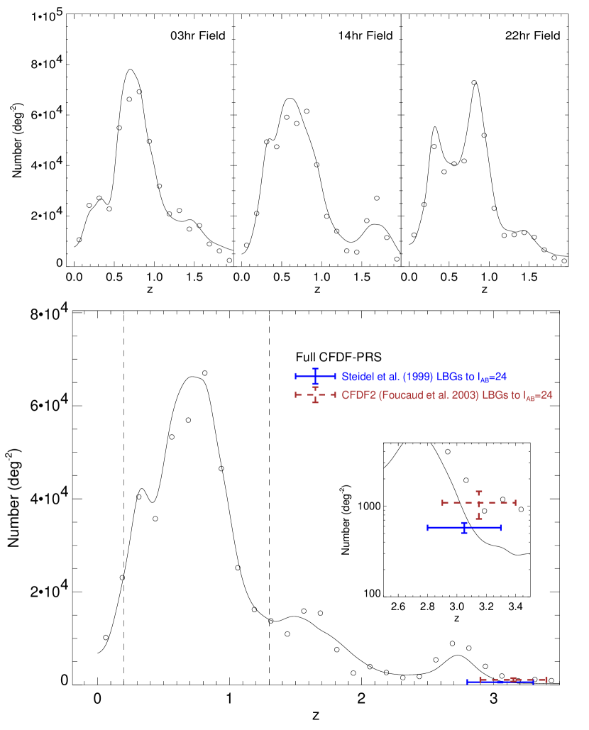
The distinct characteristics of each field, as well as the evolution from the brighter $18.5\leq I_{\mbox{\small{AB}}}\leq 22.5$ sample are discussed below.

5.3. $N(z)$ as a Function of Survey Depth

Comparing Figures 9 and 10, we see several trends in the transition from the CFRS depth to the CFDF–PRS limit of $I_{\mbox{\small{AB}}}\sim 24$. As expected, the $z>1$ sample grows as a fraction of the general population, from $\sim 9\%$ to $\sim 30\%$, while the median redshift increases from $\left<z\right>\sim 0.6$ to $\left<z\right>\sim 0.8$. Despite the smoothing effects of photometric redshift errors, discrete structures in redshift space are still clearly seen. In this Section we give a brief description of the evolution of these structures in each field with survey depth. It is interesting to note that these field–to–field differences remain significant at the full survey depth, even on 30′ scales.

5.3.1 03hr Field (RA: $03^{h}03^{m}00^{s}$   DEC: $+00\arcdeg 09\arcmin 00\arcsec$)

The 03hr field has considerable structure at $0.6\lesssim z\lesssim 0.7$, including a probable cluster near the middle of the field. This is confirmed in the CFRS spectroscopic catalog which contains at least two physical associations of galaxies, each with about 15 galaxies within $dz\leq 0.025$ of systemic redshifts of $z\sim 0.605$ and $z\sim 0.702$. Interestingly, the CFRS did not cover the probable cluster (it being outside their survey area), but its presence strongly influenced the large scale structure they observed in this field. In the CFDF–PRS these two redshift space structures influence the redshift distribution in this field down to $I_{\mbox{\small{AB}}}=24$, resulting in a relative paucity of galaxies at $0.3\lesssim z\lesssim 0.5$, compared with the other fields and with the combined redshift distribution.

5.3.2 14hr Field (RA: $14^{h}17^{m}10^{s}$   DEC: $+52\arcdeg 24\arcmin 43\arcsec$)

The 14hr field (Groth Strip) is one of the best studied extragalactic fields (e.g. Groth et al., 1994; Lilly et al., 1995a; Steidel et al., 2003). It is the most normal, in some sense, of our three fields. The picket fence structure observed in the CFRS has been smoothed out by the photometric redshift errors, while the thirtyfold increase in area provided by the CFDF–PRS has reduced the cosmic variance, leaving a relatively smooth, single–peaked, roughly Gaussian redshift distribution for $z\leq 1.3$. This distribution does not change appreciably in shape to $I_{\mbox{\small{AB}}}=24$, aside from steady increases in median redshift and number density. However, at $z\sim 1.8$ we observe a second peak arise in $N(z)$ as we push to fainter magnitudes. Visual inspection of the galaxies involved indicates nothing unusual — they are entirely likely to be at the photometric redshift. However as this peak is outside our trusted redshift range of $0.2\leq z\leq 1.3$ we defer a detailed study of it until wide–field infrared imaging or spectroscopic redshifts are available.

The DEEP2 (Davis et al., 2003) redshift survey is targeting this field with the aim of obtaining 5000 redshifts to $I_{\mbox{\small{AB}}}<24.5$. As such, it will perform a valuable check on the results presented here.

5.3.3 22hr Field (RA: $22^{h}17^{m}48^{s}$   DEC: $+00\arcdeg 17\arcmin 13\arcsec$)

The 22hr field is perhaps the most interesting of the three. There is a large overdensity at $z\sim 0.3$ observed in both the CFRS and the CFDF–PRS to the CFRS limit of $I_{\mbox{\small{AB}}}\leq 22.5$. Between $22.5\leq I_{\mbox{\small{AB}}}\leq 24$ the situation changes dramatically, and a broad peak at $z\sim 0.8$ (the median redshift at this depth) emerges. The shape of $N(z)$ in this magnitude interval is quite similar to that in the 03hr field, albeit at slightly higher redshift. As the sample selection deepens from $18.5\leq I_{\mbox{\small{AB}}}\leq 22.5$ to $18.5\leq I_{\mbox{\small{AB}}}\leq 24$ the relative sizes of the $z\sim 0.3$ and $z\sim 0.8$ peaks completely reverse. In addition, there is evidence for a substantial galaxy overdensity at $z\sim 1$.

The VIRMOS–VLT deep spectroscopic survey (VVDS, Le Fèvre et al., 2003) will obtain tens of thousands of spectroscopic redshifts to $I_{\mbox{\small{AB}}}<22.5$ over 3.6 deg² in this field. Given the relatively bright magnitude limit, it will be instructive to see whether this is sufficient area to obtain a redshift distribution unbiased by the $z\sim 0.3$ structure seen in our data, and whether it will be deep enough to confirm the existence of considerable structure at $z\sim 1$.

5.4. Median Redshifts in the CFDF–PRS

Several statistical studies including the extraction of cosmological parameters in weak lensing shear studies only require, to good approximation, the low–order moments of the galaxy population (e.g. Bernardeau et al., 1997). Due to the sensitivity of the mean to occasional systematic photometric redshift errors, we instead compute median redshifts in various cumulative and differential magnitude bins. Tomographic weak lensing studies can use such information to improve the measurement of cosmological parameters by up to an order of magnitude (Hu, 1999).

While the median is a robust statistic, there are two sources of error which may nevertheless bias it in a photometric redshift survey such as CFDF–PRS. The first, cosmic variance, applies equally well to traditional spectroscopic surveys. It is a sort of random error, in the sense that it can be minimized by observing many fields. Following Efstathiou et al. (1991) (see also Groth and Peebles 1977, Somerville et al. 2003), we calculate the fractional variance in the counts due to small–scale clustering to be $\sigma^{2}\approx 2\%$, or $\sigma\approx 15\%$. This agrees quite well with the maximum empirically measured field–to–field variations given in Tables 3 and 4, although the uncertainties in the latter estimates are themselves of order $\sqrt{2/(n-1)}=100\%$ for our $n=3$ fields (Pen et al., 2003). The Poisson noise is negligible for samples as large as this and therefore, in the absence of systematics, the cosmic variance is expected to dominate the error budget.

The second source of error, catastrophic failures of the photometric redshift method caused by redshift aliasing in low S/N photometric data, is systematic in nature. The simulations of Section 4.3 indicate the redshift regime which is free of such aliasing ($0.2\leq z\leq 1.3$), and we in fact use this convergence region in fitting our redshift distributions in the next Section. However, catastrophic errors do take place outside this convergence region, as is clear from Figure 5, and we would like to investigate the effect of these errors on the median of the full sample.

We make two estimates of the systematic error due to redshift aliasing. The first, and most conservative, adopts the worst–case scenario that all redshifts outside the convergence region are untrustworthy, which from Section §3.3 we know is not the case. We compute the median omitting all objects outside the $0\leq z\leq 1.3$ convergence region, using two one–sided redshift cuts (i.e. $z\geq 0.2$ and $z\leq 1.3$) to estimate the asymmetric maximal systematic error possible in the survey. A more realistic estimate of the systematic error is estimated via simulations like those described in Section §3.2. The CFDF–PRS $I_{\mbox{\small{AB}}}$ and $R_{\mbox{\small{AB}}}$ median redshifts, along with all of the error estimates are listed in Tables 3 and 4, respectively. We also provide in these Tables median redshifts in differential (half) magnitude bins. Given these results, simple apparent magnitudes cuts in future imaging surveys can be used as proxies for photometric redshift information in tomographic weak lensing studies.

Table 3$I_{\mbox{\tiny{AB}}}$ Median Redshifts in the CFDF–PRS

						Potential Systematic Effects
			Random Errors			due to Redshift Aliasing
			1–$\sigma$	1–$\sigma$		$\Delta_{\mbox{best}}$	$\Delta_{\mbox{best}}$	$\Delta_{\mbox{max}}$	$\Delta_{\mbox{max}}$
Mag Range	$\langle I_{\mbox{\tiny{AB}}}\rangle$	$\langle z\rangle$	Bootstrap	Field–to–Field		($z=3\rightarrow 0$)	($z=0\rightarrow 3$)	($z\leq 1.3$)	($z\geq 0.2$)
$18.5\leq I_{\mbox{\tiny{AB}}}\leq 20.5$	$19.88$	$0.38$	$0.006$	$0.035$		$-0.00$	$0.00$	$-0.01$	$0.02$
$18.5\leq I_{\mbox{\tiny{AB}}}\leq 21.0$	$20.36$	$0.43$	$0.006$	$0.065$		$-0.00$	$0.01$	$-0.01$	$0.03$
$18.5\leq I_{\mbox{\tiny{AB}}}\leq 21.5$	$20.79$	$0.49$	$0.007$	$0.075$		$-0.00$	$0.01$	$-0.02$	$0.02$
$18.5\leq I_{\mbox{\tiny{AB}}}\leq 22.0$	$21.23$	$0.54$	$0.006$	$0.070$		$-0.00$	$0.01$	$-0.01$	$0.02$
$18.5\leq I_{\mbox{\tiny{AB}}}\leq 22.5$	$21.68$	$0.59$	$0.004$	$0.055$		$-0.00$	$0.01$	$-0.02$	$0.02$
$18.5\leq I_{\mbox{\tiny{AB}}}\leq 23.0$	$22.11$	$0.64$	$0.004$	$0.031$		$-0.00$	$0.01$	$-0.03$	$0.02$
$18.5\leq I_{\mbox{\tiny{AB}}}\leq 23.5$	$22.59$	$0.71$	$0.005$	$0.040$		$-0.01$	$0.01$	$-0.06$	$0.01$
$18.5\leq I_{\mbox{\tiny{AB}}}\leq 24.0$	$23.11$	$0.77$	$0.005$	$0.049$		$-0.01$	$0.02$	$-0.09$	$0.02$
$18.5\leq I_{\mbox{\tiny{AB}}}\leq 19.0$	$18.76$	$0.30$	$0.010$	$0.023$		$-0.00$	$0.01$	$-0.01$	$0.03$
$19.0\leq I_{\mbox{\tiny{AB}}}\leq 19.5$	$19.27$	$0.32$	$0.008$	$0.010$		$-0.00$	$0.00$	$-0.01$	$0.02$
$19.5\leq I_{\mbox{\tiny{AB}}}\leq 20.0$	$19.79$	$0.39$	$0.011$	$0.023$		$-0.00$	$0.01$	$-0.01$	$0.02$
$20.0\leq I_{\mbox{\tiny{AB}}}\leq 20.5$	$20.28$	$0.43$	$0.011$	$0.085$		$-0.00$	$0.01$	$-0.01$	$0.03$
$20.5\leq I_{\mbox{\tiny{AB}}}\leq 21.0$	$20.79$	$0.52$	$0.010$	$0.072$		$-0.00$	$0.00$	$-0.01$	$0.02$
$21.0\leq I_{\mbox{\tiny{AB}}}\leq 21.5$	$21.28$	$0.58$	$0.007$	$0.050$		$-0.00$	$0.01$	$-0.01$	$0.01$
$21.5\leq I_{\mbox{\tiny{AB}}}\leq 22.0$	$21.78$	$0.63$	$0.007$	$0.040$		$-0.00$	$0.01$	$-0.02$	$0.01$
$22.0\leq I_{\mbox{\tiny{AB}}}\leq 22.5$	$22.27$	$0.71$	$0.006$	$0.036$		$-0.01$	$0.00$	$-0.03$	$0.01$
$22.5\leq I_{\mbox{\tiny{AB}}}\leq 23.0$	$22.77$	$0.78$	$0.007$	$0.031$		$-0.00$	$0.01$	$-0.06$	$0.02$
$23.0\leq I_{\mbox{\tiny{AB}}}\leq 23.5$	$23.27$	$0.89$	$0.007$	$0.031$		$-0.01$	$0.01$	$-0.11$	$0.02$
$23.5\leq I_{\mbox{\tiny{AB}}}\leq 24.0$	$23.78$	$1.03$	$0.008$	$0.061$		$-0.04$	$0.02$	$-0.23$	$0.03$
$24.0\leq I_{\mbox{\tiny{AB}}}\leq 24.5$	$24.27$	$1.26$	$0.010$	$0.083$		$-0.13$	$0.04$	$-0.47$	$0.06$

Note. — Errors of $\pm 0.00$ are smaller than the photometric redshift resolution of $0.01$.

Table 4$R_{\mbox{\tiny{AB}}}$ Median Redshifts in the CFDF–PRS

						Potential Systematic Effects
			Random Errors			due to Redshift Aliasing
			1–$\sigma$	1–$\sigma$		$\Delta_{\mbox{best}}$	$\Delta_{\mbox{best}}$	$\Delta_{\mbox{max}}$	$\Delta_{\mbox{max}}$
Mag Range	$\langle R_{\mbox{\tiny{AB}}}\rangle$	$\langle z\rangle$	Bootstrap	Field–to–Field		($z=3\rightarrow 0$)	($z=0\rightarrow 3$)	($z\leq 1.3$)	($z\geq 0.2$)
$18.5\leq R_{\mbox{\tiny{AB}}}\leq 20.5$	$19.79$	$0.34$	$0.006$	$0.012$		$-0.00$	$0.01$	$-0.01$	$0.02$
$18.5\leq R_{\mbox{\tiny{AB}}}\leq 21.0$	$20.26$	$0.36$	$0.005$	$0.012$		$-0.01$	$0.00$	$-0.01$	$0.02$
$18.5\leq R_{\mbox{\tiny{AB}}}\leq 21.5$	$20.71$	$0.38$	$0.005$	$0.032$		$-0.00$	$0.01$	$-0.01$	$0.03$
$18.5\leq R_{\mbox{\tiny{AB}}}\leq 22.0$	$21.16$	$0.42$	$0.005$	$0.065$		$-0.00$	$0.01$	$-0.01$	$0.03$
$18.5\leq R_{\mbox{\tiny{AB}}}\leq 22.5$	$21.65$	$0.47$	$0.005$	$0.075$		$-0.01$	$0.01$	$-0.02$	$0.02$
$18.5\leq R_{\mbox{\tiny{AB}}}\leq 23.0$	$22.12$	$0.52$	$0.005$	$0.075$		$-0.00$	$0.01$	$-0.02$	$0.02$
$18.5\leq R_{\mbox{\tiny{AB}}}\leq 23.5$	$22.59$	$0.57$	$0.004$	$0.065$		$-0.00$	$0.01$	$-0.02$	$0.02$
$18.5\leq R_{\mbox{\tiny{AB}}}\leq 24.0$	$23.09$	$0.63$	$0.005$	$0.042$		$-0.00$	$0.02$	$-0.04$	$0.02$
$18.5\leq R_{\mbox{\tiny{AB}}}\leq 24.5$	$23.61$	$0.71$	$0.003$	$0.030$		$-0.01$	$0.02$	$-0.09$	$0.02$
$18.5\leq R_{\mbox{\tiny{AB}}}\leq 19.0$	$18.78$	$0.33$	$0.011$	$0.040$		$-0.00$	$0.01$	$-0.02$	$0.03$
$19.0\leq R_{\mbox{\tiny{AB}}}\leq 19.5$	$19.29$	$0.32$	$0.009$	$0.023$		$-0.00$	$0.00$	$-0.01$	$0.02$
$19.5\leq R_{\mbox{\tiny{AB}}}\leq 20.0$	$19.78$	$0.33$	$0.009$	$0.010$		$-0.00$	$0.00$	$-0.01$	$0.02$
$20.0\leq R_{\mbox{\tiny{AB}}}\leq 20.5$	$20.29$	$0.37$	$0.009$	$0.021$		$-0.00$	$0.00$	$-0.01$	$0.02$
$20.5\leq R_{\mbox{\tiny{AB}}}\leq 21.0$	$20.78$	$0.39$	$0.009$	$0.065$		$-0.00$	$0.01$	$-0.01$	$0.03$
$21.0\leq R_{\mbox{\tiny{AB}}}\leq 21.5$	$21.27$	$0.44$	$0.009$	$0.068$		$-0.00$	$0.01$	$-0.00$	$0.03$
$21.5\leq R_{\mbox{\tiny{AB}}}\leq 22.0$	$21.78$	$0.52$	$0.008$	$0.085$		$-0.00$	$0.01$	$-0.01$	$0.01$
$22.0\leq R_{\mbox{\tiny{AB}}}\leq 22.5$	$22.28$	$0.55$	$0.006$	$0.076$		$-0.00$	$0.01$	$-0.01$	$0.02$
$22.5\leq R_{\mbox{\tiny{AB}}}\leq 23.0$	$22.78$	$0.64$	$0.006$	$0.025$		$-0.00$	$0.00$	$-0.02$	$0.01$
$23.0\leq R_{\mbox{\tiny{AB}}}\leq 23.5$	$23.28$	$0.73$	$0.006$	$0.023$		$-0.01$	$0.01$	$-0.05$	$0.01$
$23.5\leq R_{\mbox{\tiny{AB}}}\leq 24.0$	$23.78$	$0.85$	$0.007$	$0.015$		$-0.02$	$0.01$	$-0.12$	$0.01$
$24.0\leq R_{\mbox{\tiny{AB}}}\leq 24.5$	$24.28$	$1.01$	$0.009$	$0.040$		$-0.04$	$0.02$	$-0.24$	$0.04$
$24.5\leq R_{\mbox{\tiny{AB}}}\leq 25.0$	$24.76$	$1.21$	$0.010$	$0.080$		$-0.11$	$0.03$	$-0.42$	$0.06$

The complete error on each median redshift consists of the random error (a quadrature sum of the bootstrap and field–to–field errors) as well as the best estimate of the asymmetric systematic errors. For the $18.5\leq I_{\mbox{\small{AB}}}\leq 24$ sample the median redshift is therefore $\langle z\rangle=0.77\pm 0.049\mbox{ (random) }\,\,^{+0.02}_{-0.01}\mbox{ (systematic)}$, where we use angle brackets to denote the median. We include median redshifts for the $24.0\leq I_{\mbox{\small{AB}}}\leq 24.5$ and $24.5\leq R_{\mbox{\small{AB}}}\leq 25.0$ samples which are formally outside our trusted magnitude range for accurate photometric redshifts, as can be seen by the sudden rise in the systematic error for these samples. Nevertheless, as the median is a reasonably robust statistic and of significant value to weak lensing studies, we tentatively include these two medians for use until deeper photometric redshift surveys become available.

An important point to realize in interpreting Tables 3 and 4 is that the errors on the medians would persist in an ideal spectroscopic survey. The random error estimates are not specific to the photometric redshift method and would be unchanged for a similar spectroscopic sample. However, the spectroscopic redshift samples published to date do not approach the combination of field size, area and depth of the present survey, and have therefore been more affected by cosmic variance. The best–estimate systematic errors would remain non–zero for the faintest magnitude limits in a spectroscopic survey, as single line redshift identifications are inherently problematic and lead to catastrophic failures for as many as $\sim 10\%$ of the galaxies (e.g. see Fernandez-Soto et al., 2002). An additional systematic uncertainty, unique to spectroscopic surveys and quite difficult to estimate, is how spectroscopic incompleteness, most severe for galaxies with weak or absent emission lines, affects the measured $N(z)$.

As is clear from the Table, the field–to–field variance dominates the error budget in all cumulative (and most differential) magnitude ranges, and as such, the accuracy of the median redshifts in the CFDF–PRS is no worse than we had undertaken a more costly spectroscopic survey. In fact, for the reasons mentioned above it may be superior.

5.5. Comparison to COMBO–17, CNOC2 and HDF Median Redshifts

In Figure 11 we compare our $R$–band median redshifts to those of the COMBO–17 (Brown et al., 2003) photometric redshift survey and the CNOC2 (Yee et al., 2000) and Cohen et al. (2000) spectroscopic redshift surveys. The median redshifts are plotted versus median $R_{\mbox{\small{AB}}}$ magnitudes which are tabulated alongside the various sample magnitude ranges in Table 4.

Figure 11.— Median redshift vs. median $R_{\mbox{\tiny{AB}}}$ magnitude in the CFDF–PRS (filled symbols), along with results for the COMBO–17 (Brown et al., 2003), CNOC2 (Yee et al., 2000) and HDF North (Cohen et al., 2000) surveys , adjusted to AB magnitudes.

Our results agree fairly well with, and are in fact intermediate between, the Combo–17 and Cohen et al. (2000) results at the bright end, where the effect of cosmic variance is most important. For the CNOC2 comparison we compute the median $R_{\mbox{\tiny{AB}}}$ magnitudes and redshifts from the published catalog for the 0223+00 patch, as well as for three unpublished patches provided to us by H. Yee. To better match the CFDF–PRS, we have limited the CNOC2 sample to $R_{\mbox{\tiny{AB}}}\geq 18.5$, used the same magnitude ranges as in the present work, and estimated the error in the median from the field–to–field variance. Between $\langle R_{\mbox{\tiny{AB}}}\rangle\sim 20$ and $\langle R_{\mbox{\tiny{AB}}}\rangle\sim 20.75$, the CNOC2 limit, the agreement is excellent. The brightest CNOC2 point, at $\langle R_{\mbox{\tiny{AB}}}\rangle>\sim 19.5$ is at somewhat lower redshift than the trend implied by our data, but within the expected cosmic variance.

At fainter magnitudes these effects are minimized and the comparison becomes more straightforward. The agreement with both the COMBO–17 and Cohen et al. (2000) surveys is excellent for all $R_{\mbox{\small{AB}}}\gtrsim 21$ within the quoted errors. For consistency, we transform the published quartile limits for the Cohen et al. (2000) sample into 1–$\sigma$ errors assuming Gaussian distributions. While we agree with the Cohen et al. (2000) median redshifts within these conservatively large error limits, our fields clearly show a lower median redshift at faint magnitudes, quite in line with the COMBO–17 results. In fact, given the strong agreement our results suggest that for ensemble statistical measurements of the galaxy population, such as the two–point correlation function, it is perhaps advantageous to employ only $\sim 6$ broad–band filters (with spectral coverage from $U$ through $Z$ bands) and image more deeply rather than adopt a brighter medium band approach with $\sim 15$ filters. While the photometric redshift error on individual galaxies is likely lower with the medium band survey strategy, broad–band photometric redshift surveys like the CFDF–PRS probe deeper down the luminosity function with little penalty on statistical measurements.

6. Representation of the CFDF–PRS Redshift Distributions

In this Section we present our redshift distributions binned in magnitude and redshift, as well as in parametrized form in various magnitude ranges. It should be noted that none of the main qualitative results of this paper change if simple maximum likelihood redshift (Peak–ML) values are used in place of the Final RLF described in Section §4.

6.1. Binned Redshift Distributions

In Tables 5 and 6 we present the measured CFDF–PRS redshift distributions, binned so as to present trustworthy information over all redshifts. Specifically, we tabulate the Final RLF $N(z)$ in redshift bins of $\Delta z=0.1$ for $z<1.3$ and much more broadly ($\Delta z=1.0$) at high redshift where the photometric redshifts are not as accurate. Our distributions are presented in $0.5$ magnitude bins, which should enable other workers to construct redshift distributions for any sample in the range $18.5\leq I_{\mbox{\small{AB}}}\leq 24$, with the obvious caveat that bright samples containing small numbers of objects have relatively larger uncertainties than deeper samples.

Table 5Binned $I_{\mbox{\tiny{AB}}}$ CFDF–PRS Redshift Distributions

			$\left<I_{\mbox{\tiny{AB}}}\right>_{\Delta m=0.5}$
$z_{l}-z_{h}$	$z$		$18.75$	$19.25$	$19.75$	$20.25$	$20.75$	$21.25$	$21.75$	$22.25$	$22.75$	$23.25$	$23.75$
$0.05-0.15$	$0.10$		$157$	$161$	$140$	$266$	$313$	$284$	$343$	$419$	$636$	$928$	$1703$
$0.15-0.25$	$0.20$		$320$	$390$	$362$	$533$	$726$	$750$	$956$	$1163$	$1395$	$1648$	$2594$
$0.25-0.35$	$0.30$		$638$	$905$	$869$	$1098$	$1316$	$1485$	$1702$	$2112$	$2080$	$2375$	$3058$
$0.35-0.45$	$0.40$		$281$	$547$	$921$	$1179$	$1404$	$1557$	$2007$	$2147$	$2207$	$2608$	$3255$
$0.45-0.55$	$0.50$		$79$	$181$	$638$	$1042$	$1718$	$1885$	$2787$	$2657$	$2961$	$3224$	$4384$
$0.55-0.65$	$0.60$		$48$	$78$	$387$	$968$	$2024$	$2665$	$3551$	$3735$	$4136$	$4544$	$5453$
$0.65-0.75$	$0.70$		$27$	$29$	$153$	$401$	$1229$	$2142$	$3355$	$4519$	$5260$	$6073$	$6573$
$0.75-0.85$	$0.80$		$10$	$10$	$44$	$162$	$562$	$1419$	$2743$	$4264$	$5526$	$7029$	$7506$
$0.85-0.95$	$0.90$		$3$	$6$	$20$	$75$	$238$	$771$	$1617$	$2967$	$4436$	$6511$	$7402$
$0.95-1.05$	$1.00$		$1$	$3$	$9$	$22$	$66$	$224$	$659$	$1506$	$2728$	$4899$	$6616$
$1.05-1.15$	$1.10$		$1$	$2$	$4$	$7$	$19$	$62$	$237$	$670$	$1448$	$2999$	$4870$
$1.15-1.25$	$1.20$		$0$	$1$	$3$	$5$	$10$	$32$	$125$	$377$	$990$	$2119$	$3764$
$1.25-2.25$	$1.75$		$0$	$1$	$2$	$2$	$5$	$16$	$62$	$199$	$512$	$1183$	$2373$
$1.75-2.75$	$2.25$		$6$	$4$	$5$	$8$	$8$	$11$	$40$	$85$	$204$	$507$	$1188$
$2.25-3.25$	$2.75$		$18$	$7$	$9$	$15$	$21$	$19$	$47$	$70$	$132$	$292$	$645$
$2.75-3.75$	$3.25$		$14$	$3$	$5$	$8$	$13$	$10$	$16$	$24$	$48$	$116$	$289$
$3.25-4.25$	$3.75$		$1$	$0$	$0$	$1$	$0$	$2$	$0$	$0$	$3$	$10$	$51$
$3.75-4.75$	$4.25$		$0$	$0$	$0$	$0$	$0$	$3$	$0$	$0$	$1$	$6$	$25$

Note. — The redshift distributions are presented in constant 0.5 magnitude bins between $18.5\leq I_{\mbox{\small{AB}}}\leq 24$, whereas the $\Delta z=0.1$ bin size in redshift is expanded to overlapping $\Delta z=1.0$ bins at $z>1.25$. In each redshift bin the number of galaxies in the $\Delta m=0.5$ magnitude range is computed as $N=\int_{z_{l}}^{z_{h}}N(z,m_{l}\leq I_{\mbox{\small{AB}}}\leq m_{h})\,dz/\int_{z_{l}}^{z_{h}}dz$, where $m_{l}=\left<I_{\mbox{\small{AB}}}\right>-0.25$, $m_{h}=\left<I_{\mbox{\small{AB}}}\right>+0.25$, and the number densities, $N$, represent the CFDF–PRS survey area of 0.4514 deg².

Table 6Binned $R_{\mbox{\tiny{AB}}}$ CFDF–PRS Redshift Distributions

			$\left<R_{\mbox{\tiny{AB}}}\right>_{\Delta m=0.5}$
$z_{l}-z_{h}$	$z$		$18.75$	$19.25$	$19.75$	$20.25$	$20.75$	$21.25$	$21.75$	$22.25$	$22.75$	$23.25$	$23.75$	$24.25$
$0.05-0.15$	$0.10$		$128$	$150$	$183$	$168$	$318$	$279$	$306$	$408$	$429$	$743$	$1051$	$1956$
$0.15-0.25$	$0.20$		$230$	$303$	$432$	$443$	$642$	$782$	$794$	$1171$	$1125$	$1499$	$1722$	$2780$
$0.25-0.35$	$0.30$		$488$	$706$	$850$	$1017$	$1243$	$1553$	$1648$	$2088$	$2004$	$2279$	$2475$	$3240$
$0.35-0.45$	$0.40$		$340$	$410$	$605$	$929$	$1244$	$1658$	$1913$	$2239$	$2224$	$2571$	$2790$	$3410$
$0.45-0.55$	$0.50$		$92$	$144$	$222$	$630$	$1016$	$1802$	$2240$	$3031$	$3096$	$3109$	$3326$	$4204$
$0.55-0.65$	$0.60$		$43$	$93$	$114$	$302$	$650$	$1587$	$2755$	$3632$	$4382$	$4292$	$4591$	$5037$
$0.65-0.75$	$0.70$		$11$	$32$	$40$	$63$	$211$	$558$	$1615$	$2618$	$4373$	$5370$	$5893$	$6135$
$0.75-0.85$	$0.80$		$2$	$8$	$9$	$13$	$43$	$97$	$502$	$1339$	$2882$	$4900$	$6216$	$7061$
$0.85-0.95$	$0.90$		$1$	$3$	$3$	$3$	$14$	$22$	$133$	$575$	$1624$	$3232$	$5092$	$6597$
$0.95-1.05$	$1.00$		$0$	$2$	$1$	$2$	$8$	$5$	$40$	$208$	$698$	$1764$	$3377$	$5318$
$1.05-1.15$	$1.10$		$0$	$1$	$0$	$2$	$4$	$1$	$17$	$80$	$312$	$874$	$2077$	$3737$
$1.15-1.25$	$1.20$		$0$	$1$	$0$	$2$	$2$	$1$	$9$	$41$	$162$	$537$	$1496$	$2955$
$1.25-2.25$	$1.75$		$0$	$0$	$1$	$1$	$1$	$1$	$9$	$27$	$101$	$384$	$1031$	$2154$
$1.75-2.75$	$2.25$		$7$	$3$	$6$	$7$	$8$	$8$	$19$	$41$	$84$	$229$	$565$	$1240$
$2.25-3.25$	$2.75$		$20$	$8$	$10$	$13$	$20$	$16$	$27$	$45$	$68$	$139$	$297$	$696$
$2.75-3.75$	$3.25$		$14$	$7$	$5$	$7$	$12$	$9$	$12$	$15$	$27$	$44$	$126$	$341$
$3.25-4.25$	$3.75$		$1$	$1$	$0$	$1$	$0$	$0$	$1$	$1$	$2$	$2$	$23$	$77$
$3.75-4.75$	$4.25$		$0$	$0$	$0$	$0$	$0$	$0$	$2$	$1$	$0$	$0$	$3$	$15$

Note. — All quantities are as in defined in Table 5, with the addition of the distribution for the $24.0<R_{\mbox{\small{AB}}}<24.5$ bin in the final column.

Figure 12.— Binned distributions (solid symbols) and best–fit parametrizations plotted along with the $18.5\leq I~{}_{\mbox{\tiny{AB}}}\leq 22.5$ and $18.5\leq I_{\mbox{\tiny{AB}}}\leq 24$ RLF redshift distributions (thin solid curves), scaled to 1 square degree. The solid thick line shows the best fitting parametrization of the main peak (Equation 4) at $z\lesssim 1.2$ (represented as a dotted curve outside the fitting range, i. e. at $z<0.375$). At $z\gtrsim 1.2$ the long–dashed curve is the best fitting model of the high redshift tail (Equation 5). The CFRS histogram is included for reference as the (dotted) histogram, where once again the dotted square represents the unidentified fraction of CFRS objects.

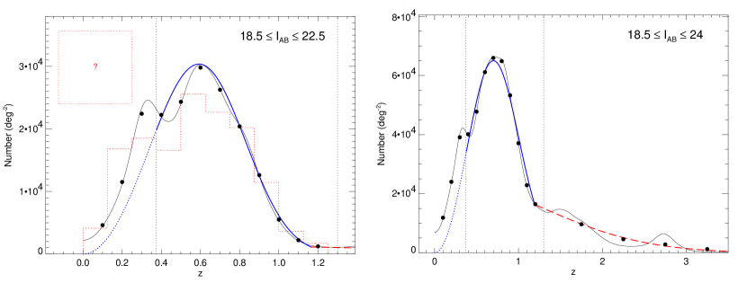
As an example, in Figure 12 we plot the binned distributions (filled symbols) for the CFRS depth of $18.5\leq I_{\mbox{\small{AB}}}\leq 22.5$ and the full CFDF–PRS depth of $18.5\leq I_{\mbox{\small{AB}}}\leq 24$ along with the full distributions (thin solid curves). The binned distributions accurately represent the data at all redshifts, although they are highly smoothed at $z>1.25$. As such our distributions should be used in this form for precision (e. g. cosmic shear) measurements.

6.2. Parametrizations of $N(z)$

For convenience we provide in this Section parametrized fits to our redshift distributions, adopting a generalization of the functional form introduced by Efstathiou et al. (1991):

$$N(z)=N_{0}\frac{\beta}{z_{0}\,\Gamma\left(\frac{1+\alpha}{\beta}\right)}\left(\frac{z}{z_{0}}\right)^{\alpha}\exp\left[-\left(\frac{z}{z_{0}}\right)^{\beta}\right]$$ (4)

These functions were fitted to our $I_{\mbox{\small{AB}}}$ and $R_{\mbox{\small{AB}}}$ redshift distributions in various magnitude ranges and the results are listed in Tables 7 and 8, respectively. We limit our fits to the redshift region $0.375\leq z\leq 1.3$, i. e. we exclude the $z\sim 0.3$ overdensity and fit the main single peak in each magnitude range.

Table 7Parametrized Fits of $I_{\mbox{\tiny{AB}}}$ CFDF–PRS Redshift Distributions

		$z\lesssim 1.2$							$z\gtrsim 1.2$
Mag Range		$N_{0}$		$z_{0}$		$\beta$			$A_{T}$	$z_{T}$	$\gamma$
$18.5\leq I_{\mbox{\tiny{AB}}}\leq 24.0$		20785	(133)	000.790	(0.008)	002.788	(0.059)		11443	1.786	2.037
$19.0\leq I_{\mbox{\tiny{AB}}}\leq 24.0$		20735	(141)	0.793	(0.009)	2.805	(0.067)		11472	1.783	2.039
$19.5\leq I_{\mbox{\tiny{AB}}}\leq 24.0$		20625	(143)	0.800	(0.008)	2.852	(0.058)		11503	1.780	2.037
$20.0\leq I_{\mbox{\tiny{AB}}}\leq 24.0$		20310	(135)	0.818	(0.009)	2.969	(0.074)		11557	1.776	2.033
$20.5\leq I_{\mbox{\tiny{AB}}}\leq 24.0$		19800	(126)	0.840	(0.008)	3.123	(0.073)		11609	1.773	2.032
$21.0\leq I_{\mbox{\tiny{AB}}}\leq 24.0$		18861	(141)	0.872	(0.007)	3.341	(0.074)		11695	1.770	2.031
$21.5\leq I_{\mbox{\tiny{AB}}}\leq 24.0$		17569	(128)	0.902	(0.007)	3.529	(0.093)		11635	1.782	2.053
$22.0\leq I_{\mbox{\tiny{AB}}}\leq 24.0$		15573	(120)	0.945	(0.008)	3.817	(0.121)		11672	1.776	2.043
$22.5\leq I_{\mbox{\tiny{AB}}}\leq 24.0$		13046	(111)	0.978	(0.009)	3.904	(0.135)		11131	1.788	2.045
$23.0\leq I_{\mbox{\tiny{AB}}}\leq 24.0$		9829	(90)	1.015	(0.008)	3.992	(0.122)		9383	1.837	2.074
$18.5\leq I_{\mbox{\tiny{AB}}}\leq 21.5$		3216	(169)	0.609	(0.010)	3.200	(0.096)		44	3.717	93.92
$18.5\leq I_{\mbox{\tiny{AB}}}\leq 22.0$		5205	(165)	0.644	(0.008)	3.175	(0.075)		109	3.460	14.55
$18.5\leq I_{\mbox{\tiny{AB}}}\leq 22.5$		7759	(186)	0.683	(0.009)	3.119	(0.068)		658	2.084	2.327
$18.5\leq I_{\mbox{\tiny{AB}}}\leq 23.0$		10979	(168)	0.720	(0.008)	3.048	(0.067)		2422	1.716	1.994
$18.5\leq I_{\mbox{\tiny{AB}}}\leq 23.5$		15293	(157)	0.760	(0.008)	2.941	(0.066)		5889	1.699	2.013
$18.5\leq I_{\mbox{\tiny{AB}}}\leq 24.0$		20785	(133)	0.790	(0.008)	2.788	(0.059)		11443	1.786	2.037

Note. — The fits are for the CFDF–PRS survey area of 0.4514 deg². At $z\lesssim 1.2$ the best–fitting parameters of Equation 4 are listed, along with bootstrap–resampled errors. At $z\gtrsim 1.2$, the parameters of fits of the form of Equation 5 are tabulated. We conservatively estimate the error in the high redshift tail to be 50%.

Table 8Parametrized Fits of $R_{\mbox{\tiny{AB}}}$ CFDF–PRS Redshift Distributions

		$z\lesssim 1.2$							$z\gtrsim 1.2$
Mag Range		$N_{0}$		$z_{0}$		$\beta$			$A_{T}$	$z_{T}$	$\gamma$
$18.5\leq R_{\mbox{\tiny{AB}}}\leq 24.0$		13446	(133)	000.662	(0.012)	002.601	(0.081)		2380	2.433	3.083
$19.0\leq R_{\mbox{\tiny{AB}}}\leq 24.0$		13379	(121)	0.667	(0.011)	2.629	(0.073)		2415	2.407	3.034
$19.5\leq R_{\mbox{\tiny{AB}}}\leq 24.0$		13288	(113)	0.673	(0.010)	2.659	(0.065)		2425	2.399	3.025
$20.0\leq R_{\mbox{\tiny{AB}}}\leq 24.0$		13151	(113)	0.681	(0.012)	2.710	(0.081)		2447	2.384	2.999
$20.5\leq R_{\mbox{\tiny{AB}}}\leq 24.0$		12859	(110)	0.701	(0.010)	2.837	(0.077)		2471	2.367	2.969
$21.0\leq R_{\mbox{\tiny{AB}}}\leq 24.0$		12429	(122)	0.725	(0.010)	2.993	(0.087)		2507	2.343	2.927
$21.5\leq R_{\mbox{\tiny{AB}}}\leq 24.0$		11659	(100)	0.761	(0.009)	3.232	(0.091)		2549	2.325	2.895
$22.0\leq R_{\mbox{\tiny{AB}}}\leq 24.0$		10532	(113)	0.796	(0.010)	3.434	(0.115)		2591	2.302	2.881
$22.5\leq R_{\mbox{\tiny{AB}}}\leq 24.0$		8896	(96)	0.848	(0.008)	3.812	(0.122)		2624	2.266	2.839
$23.0\leq R_{\mbox{\tiny{AB}}}\leq 24.0$		6661	(78)	0.894	(0.010)	4.036	(0.153)		2532	2.228	2.770
$18.5\leq R_{\mbox{\tiny{AB}}}\leq 22.0$		2992	(170)	0.538	(0.011)	3.140	(0.111)		28	3.716	76.46
$18.5\leq R_{\mbox{\tiny{AB}}}\leq 22.5$		4607	(150)	0.567	(0.010)	3.116	(0.084)		70	3.670	45.30
$18.5\leq R_{\mbox{\tiny{AB}}}\leq 23.0$		6800	(150)	0.602	(0.011)	3.007	(0.083)		186	3.432	13.82
$18.5\leq R_{\mbox{\tiny{AB}}}\leq 23.5$		9632	(145)	0.634	(0.013)	2.825	(0.098)		612	2.982	5.643
$18.5\leq R_{\mbox{\tiny{AB}}}\leq 24.0$		13446	(133)	0.662	(0.012)	2.601	(0.081)		2380	2.433	3.083
$18.5\leq R_{\mbox{\tiny{AB}}}\leq 24.5$		18656	(146)	0.665	(0.012)	2.309	(0.060)		5930	2.337	2.778

Note. — All quantities are defined as in Table 7. For the $R_{\mbox{\small{AB}}}$ sample we also provide a fit for the $18.5\leq R_{\mbox{\small{AB}}}\leq 24.5$ magnitude range.

Our fitting technique consists of minimizing the Kolmogorov–Smirnov distance $D$ between the cumulative distribution functions of the model and Final RLF method redshift distributions over the allowed redshift range. The full three parameter fits [$z_{0},\,\alpha,\,\beta]$ have $\alpha$ values very close to the commonly used value of 2.0 (see, e.g., Efstathiou et al., 1991), expected on geometric arguments for a flat average luminosity function. Without significantly compromising the accuracy of the fits, we therefore reduce the dimensionality of the analysis by setting $\alpha\equiv 2.0$. The 1–$\sigma$ single parameter errors in $z_{0}$ and $\beta$, listed in the Tables, are estimated via 100 bootstrap resamplings (with repetitions) of the CFDF–PRS catalog, and subsequent recalculation of the redshift distributions using the Full–RLF method. The separately determined absolute number densities, $N_{0}$, along with bootstrap resampled errors are also listed in the Tables.

We found Equation 4 to be a sensible model for $N(z)$ up to the CFRS depth ($I_{\mbox{\small{AB}}}\sim 22.5$), but at fainter magnitudes it fails to simultaneously model the main $z\lesssim 1$ peak and the increasing high redshift tail (at $I_{\mbox{\small{AB}}}\lesssim 24$ the fraction of $z>1$ galaxies is approximately 30%). We therefore limit its application to the $z\lesssim 1.2$ regime and fit the $z\gtrsim 1.2$ tail of the distribution with a decaying exponential,

$$N(z)=A_{T}\exp\left[-\left(\frac{z}{z_{T}}\right)^{\gamma}\right].$$ (5)

Note that this equation is not fitted to the the Final RLF $N(z)$ but rather to the binned distributions calculated from Tables 5 and 6. The transition between Equations 4 and 5 is always very close to $z\approx 1.2$, but to produce a continuous parametrization should in general be taken to be the redshift at which the two parametrizations intersect.

For the high redshift tail the dominant errors are likely systematic in nature, coming from the photometric redshift algorithm operating in a redshift and magnitude regime where the convergence properties are highly uncertain. Without a large, deep spectroscopic comparison sample at $1<z<3$ it is difficult to assess these errors in a meaningful way. In the present work we conservatively assign a maximum uncertainty of 50% to the fit in the $z\gtrsim 1.3$ regime. Examples of the fits are shown in Figure 12 for the $18.5\leq I_{\mbox{\tiny{AB}}}\leq 22.5$ and $18.5\leq I_{\mbox{\tiny{AB}}}\leq 24.0$ samples. The solid, thick curve is the best fitting parametrization of the form of Equation 4 within the $0.375\leq z\leq 1.3$ fitting region, although it is likely correct at $z<0.375$ (dotted curve) due to the constraint at $z=0$. At $z\gtrsim 1.2$ the best–fit parametrization of the form of Equation 5 is represented by the long–dashed line. Taken together the full redshift range is well parametrized by these functions.

7. Summary

We have introduced a new technique to compute $N(z)$ in which the full photometric redshift likelihood functions for each galaxy are incorporated to better reproduce the correct underlying redshift distribution. Direct summation of the likelihoods produces the Bayesian prior which accounts for the fact that all redshifts are not a priori equally likely. No information external to the survey is used in the Bayesian technique, rather we iterate within our own dataset. We have presented Monte Carlo simulations which prove the validity of the technique and demonstrate that it is a significant improvement over previous methods.

Our highly accurate photometric redshifts, calibrated using hundreds of spectroscopic CFRS galaxies, have typical dispersions of only $\sigma/(1+z)\lesssim 0.06$ to $I_{\mbox{\small{AB}}}=24$ for $z\leq 1.3$. Our large field sizes ($30\arcmin$) and multiple, widely separated lines of sight produce redshift distributions far less affected by cosmic variance than previous surveys of similar depth. We compute $I_{\mbox{\small{AB}}}$ and $R_{\mbox{\small{AB}}}$ median redshifts, as a function of limiting magnitude and in differential magnitude bins, with an error budget consisting of bootstrap resampled random errors, field–to–field variance and an empirical estimate of the systematic errors due to photometric redshift aliasing. We present our $I_{\mbox{\small{AB}}}$ and $R_{\mbox{\small{AB}}}$ redshift distributions in tabular form and provide parametrized fits with errors estimated from bootstrap resampling.

This work confirms that in the redshift regimes in which multicolor imaging surveys have appropriate wavelength coverage and depth, the errors in photometric redshifts (conservatively $\Delta z/(1+z)\lesssim 0.1$) are not the limiting factor in an accurate determination of $N(z)$. In addition, we have verified that the systematic errors inherent in the method are secondary to cosmic variance in the overall error budget. Sparsely sampled spectroscopic or wide-field photometric redshift surveys containing dozens of effectively independent fields will be required to significantly improve upon the present results.

Appendix A Convergence Properties

This Appendix presents some of the tests conducted, beyond the Monte Carlo simulations presented in Section 4.3, to determine the redshift and S/N ranges for which the new method converges.

A.1. Formalism

Generalizing Equation 2 to include a single prior, $P(z)$, for a given sample

$${\cal N}(z)=P(z)\sum_{i}\frac{{\cal L}_{i}(z)}{\int_{0}^{\infty}P(z)\,{\cal L}_{i}(z)\,dz},$$ (A1)

we see that the correct prior is the one for which ${\cal N}(z)=N(z)$ (i. e. we recover the correct underlying redshift distribution). This leads to the following integral equation for $P(z)$:

$$P(z)=N(z)\left(\sum_{i}\frac{{\cal L}_{i}(z)}{\int_{0}^{\infty}P(z)\,{\cal L}_{i}(z)\,dz}\right)^{-1},$$ (A2)

which can be solved by iteration. Note that the functional form of the ideal prior depends on the likelihood functions, as expected since at very low S/N (reflected in the likelihoods) the method should fail. Viewing the prior as expressing a change of coordinates to a space in which the galaxy distribution is flat, one might expect the prior to be similar to $N(z)$. Therefore, we can use simulations to determine the redshift and S/N regimes in which taking $P(z)=N(z)$ produces the correct answer (i.e. ${\cal N}(z)=N(z)$). It is straightforward to show that this requires

$$\eta\equiv\sum_{i}\frac{{\cal L}_{i}(z)}{\int_{0}^{\infty}N(z)\,{\cal L}_{i}(z)\,dz}=1$$ (A3)

When this equation is satisfied, using $N(z)$ as the prior is strictly correct. Although in general $N(z)$ is not known a priori, assuming that $N^{0}(z)$ from Equation 2 is a reasonable approximation to $N(z)$, one might still expect that

$$\eta^{0}\equiv\sum_{i}\frac{{\cal L}_{i}(z)}{\int_{0}^{\infty}N^{0}(z)\,{\cal L}_{i}(z)\,dz}\approx 1$$ (A4)

is a valid convergence criterion.

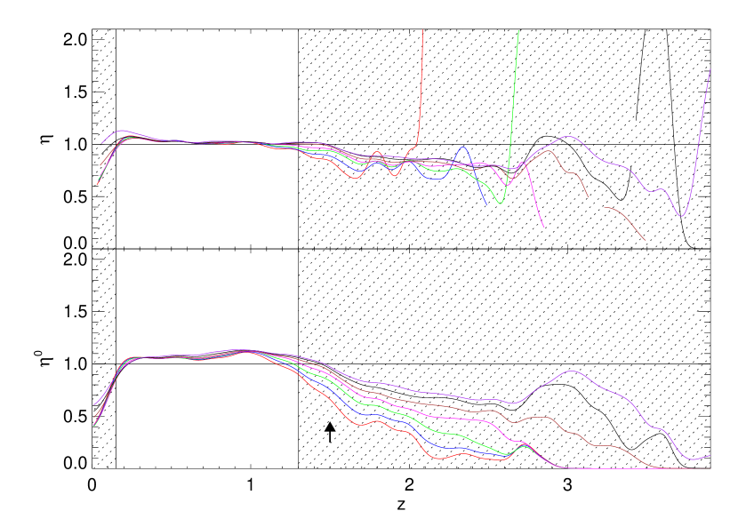
In the CFDF–PRS we set a conservative $I$–band S/N minimum of 10, about $I_{\mbox{\small{AB}}}\sim 24$, based on a direct calculation of the convergence criteria of Equations A3 and A4 (shown in Figure 13), as well as the results of the Monte Carlo simulations described in the text. The redshift range over which the method is most reliable to this depth, apparent from Figure 13, is $0.2\lesssim z\lesssim 1.3$, corresponding to values of $\eta$ and $\eta^{0}$ within 10%–15% of unity. This redshift range is in very good agreement with the predictions for our filter set (Brodwin et al., 1999).

Figure 13.— Convergence criteria $\eta$ and $\eta^{0}$ of Equations A3 and A4, calculated in the Monte Carlo simulation of Section 4.3. The unshaded region between $0.2<z<1.3$ is identified as the most trustworthy for recovering the underlying redshift distributions for magnitude limited samples down to $I_{\mbox{\tiny{AB}}}\sim 24$. Nevertheless, the redshift distribution can also be measured outside of this redshift range, though slightly less accurately, as shown in the next Section. The curves represent samples down to limiting magnitudes of $I_{\mbox{\tiny{AB}}}\leq 22.5$ (directly above arrow), rising to $I_{\mbox{\tiny{AB}}}\leq 24$ in increments of 0.25 magnitudes. The curves in the top panel are undefined where $N(z)=0$ for bright magnitude limits at high redshift. The smoothing effect of the photometric redshift errors prevents this occurrence in the lower panel.

References

- Benítez (2000) Benítez, N. 2000, ApJ, 536, 571
- Bernardeau et al. (1997) Bernardeau, F., van Waerbeke, L., and Mellier, Y. 1997, A&A, 322, 1
- Bertin and Arnouts (1996) Bertin, E. and Arnouts, S. 1996, A&AS, 117, 393
- Blanton et al. (2003) Blanton, M. R., et al. 2003, ApJ, 592, 819
- Brodwin (2004) Brodwin, M. 2004, PhD thesis, University of Toronto
- Brodwin et al. (1999) Brodwin, M., Lilly, S., and Crampton, D. 1999, in ASP Conf. Ser. 191, Photometric Redshifts and the Detection of High Redshift Galaxies, ed. Weymann, R. J. et al. (San Francisco: ASP), 105
- Brown et al. (2003) Brown, M. L., Taylor, A. N., Bacon, D. J., Gray, M. E., Dye, S., Meisenheimer, K., and Wolf, C. 2003, MNRAS, 341, 100
- Cohen et al. (2000) Cohen, J. G., Hogg, D. W., Blandford, R., Cowie, L. L., Hu, E., Songaila, A., Shopbell, P., and Richberg, K. 2000, ApJ, 538, 29
- Coleman et al. (1980) Coleman, G. D., Wu, C.-C., and Weedman, D. W. 1980, ApJS, 43, 393
- Colless et al. (2001) Colless, M., et al. 2001, MNRAS, 328, 1039
- Connolly et al. (1997) Connolly, A. J., Szalay, A. S., Dickinson, M., Subbarao, M. U., and Brunner, R. J. 1997, ApJ, 486, L11
- Crampton et al. (1995) Crampton, D., Le Fèvre, O., Lilly, S. J., and Hammer, F. 1995, ApJ, 455, 96 (CFRS5)
- Csabai et al. (2003) Csabai, I., et al. 2003, AJ, 125, 580
- Davis et al. (2003) Davis, M., et al. 2003, in Proceedings of the SPIE, Vol. 4834, Discoveries and Research Prospects from 6- to 10-Meter-Class Telescopes II, ed. Guhathakurta, P., 161
- Efstathiou et al. (1991) Efstathiou, G., Bernstein, G., Tyson, J. A., Katz, N., and Guhathakurta, P. 1991, ApJ 380, L47
- Fernández-Soto et al. (1999) Fernández-Soto, A., Lanzetta, K. M., and Yahil, A. 1999, ApJ, 513, 34
- Fernandez-Soto et al. (2002) Fernandez-Soto, A., Lanzetta, K. M., Chen, H.-W., Levine, B., and Yahata, N. 2002, MNRAS, 330, 889
- Fontana et al. (2000) Fontana, A., D’Odorico, S., Poli, F., Giallongo, E., Arnouts, S., Cristiani, S., Moorwood, A., and Saracco, P. 2000, AJ, 120, 220
- Foucaud et al. (2003) Foucaud, S., McCracken, H. J., Le Fèvre, O., Arnouts, S., Brodwin, M., Lilly, S. J., Crampton, D., and Mellier, Y. 2003, A&A, 409, 835 (CFDF2)
- Gehrels (1986) Gehrels, N. 1986, ApJ, 303, 336
- Groth et al. (1994) Groth, E. J., Kristian, J. A., Lynds, R., O’Neil, E. J., Balsano, R., Rhodes, J., and WFPC-1 IDT 1994, BAAS, 26, 1403
- Groth and Peebles (1977) Groth, E. J. and Peebles, P. J. E. 1977, ApJ, 217, 385
- Hu (1999) Hu, W. 1999, ApJ, 522, L21
- Kaiser and Peacock (1991) Kaiser, N. and Peacock, J. A. 1991, ApJ, 379, 482
- Kinney et al. (1996) Kinney, A. L., Calzetti, D., Bohlin, R. C., McQuade, K., Storchi–Bergmann, T., and Schmitt, H. R. 1996, ApJ, 467, 38
- Le Fèvre et al. (1995) Le Fèvre, O., Crampton, D., Lilly, S. J., Hammer, F., and Tresse, L. 1995, ApJ 455, 60
- Le Fèvre et al. (2003) Le Fèvre, O., et al. 2003, A&A, submitted (astro–ph/0306252)
- Lilly et al. (1995a) Lilly, S. J., Hammer, F., Le Fèvre, O., and Crampton, D. 1995a, ApJ, 455, 75
- Lilly et al. (1995b) Lilly, S. J., Le Fèvre, O., Crampton, D., Hammer, F., and Tresse, L. 1995b, ApJ, 455, 50
- Lin et al. (1999) Lin, H., Yee, H. K. C., Carlberg, R. G., Morris, S. L., Sawicki, M., Patton, D. R., Wirth, G., and Shepherd, C. W. 1999, ApJ, 518, 533
- Madau (1995) Madau, P. 1995, ApJ, 441, 18
- McCracken et al. (2001) McCracken, H. J., Le Fèvre, O., Brodwin, M., Foucaud, S., Lilly, S. J., Crampton, D., and Mellier, Y. 2001, A&A, 376, 756 (CFDF1)
- Norberg et al. (2002a) Norberg, P., et al. 2002a, MNRAS, 332, 827
- Norberg et al. (2002b) Norberg, P., et al. 2002b, MNRAS, 336, 907
- Pen et al. (2003) Pen, U., Lu, T., van Waerbeke, L., and Mellier, Y. 2003, MNRAS, 346, 994
- Sawicki et al. (1997) Sawicki, M. J., Lin, H., and Yee, H. K. C. 1997, AJ, 113, 1
- Somerville et al. (2003) Somerville, R. S., Lee, K., Ferguson, H. C., Gardner, J. P., Moustakas, L. A., and Giavalisco, M. 2003, ApJ, in press (astro–ph/0309071)
- Spergel et al. (2003) Spergel, D. N., et al. 2003, ApJS, 148, 175
- Steidel et al. (1999) Steidel, C. C., Adelberger, K. L., Giavalisco, M., Dickinson, M., and Pettini, M. 1999, ApJ, 519, 1
- Steidel et al. (2003) Steidel, C. C., Adelberger, K. L., Shapley, A. E., Pettini, M., Dickinson, M., and Giavalisco, M. 2003, ApJ, 592, 728
- Steidel et al. (1996) Steidel, C. C., Giavalisco, M., Pettini, M., Dickinson, M., and Adelberger, K. L. 1996, ApJ, 462, L17
- Szalay et al. (1999) Szalay, A. S., Connolly, A. J., and Szokoly, G. P. 1999, AJ, 117, 68
- Yee et al. (2000) Yee, H. K. C., et al. 2000, ApJS, 129, 475
- York et al. (2000) York, D. G., et al. 2000, AJ, 120, 1579
- Zehavi et al. (2002) Zehavi, I., et al. 2002, ApJ, 571, 172