A dynamical model for the distribution of dark matter and gas in galaxy clusters

Abstract

Using the results of an extended set of high-resolution non-radiative hydrodynamic simulations of galaxy clusters we obtain simple analytic formulae for the dark matter and hot gas distribution, in the spherical approximation. Starting from the dark matter phase-space radial density distribution, we derive fits for the dark matter density, velocity dispersion and velocity anisotropy. We use these models to test the dynamical equilibrium hypothesis through the Jeans equation: we find that this is satisfied to good accuracy by our simulated clusters inside their virial radii. This result also show that our fits constitute a self-consistent dynamical model for these systems.

We then extend our analysis to the hot gas component, obtaining analytic fits for the gas density, temperature and velocity structure, with no further hypothesis on the gas dynamical status or state equation. Gas and dark matter show similar density profiles down to $\approx 0.06R_{\rm v}$ (with $R_{\rm v}$ the virial radius), while at smaller radii the gas flattens producing a central core. Gas temperatures are almost isothermal out to roughly $0.2R_{\rm v}$, then steeply decrease reaching at the virial radius a value almost a factor of two lower. We find that the gas is not at rest inside $R_{\rm v}$: velocity dispersions are increasing functions of the radius, motions are isotropic to slightly tangential, and contribute non-negligibly to the total pressure support. We test this model using a generalization of the hydrostatic equilibrium equation, where the gas motion is properly taken into account. Again we find that the fits provide an accurate description of the system: the hot gas is in equilibrium and is a good tracer the overall cluster potential if all terms (density, temperature and velocity) are taken into account, while simpler assumptions cause systematic mass underestimates. In particular, we find that using the so-called $\beta$-model underestimates the true cluster mass by up to 50 per cent at large radii. We also find that, if gas velocities are neglected, then a simple isothermal model fares better at large radii than a non-isothermal one.

The shape of the gas density profile at small radii is at least partially explained by the gas expansion caused by energy transfer from dark matter during the collapse. In fact, when gas bulk energy is also considered, gas and dark matter are in energy equipartition in the final system at radii $r>0.1R_{\rm v}$, while at smaller radii the gas is hotter than the dark matter. This energy unbalance is also probably the reason of the further global halo compression compared to a pure collisionless collapse, which we point out by comparing the dark matter and total density profiles of our hydro-simulated clusters with a set of identical - but pure N-body - ones. The compression has the effect of rising the mean concentration by an amount of roughly 10 per cent.

1 Introduction

Galaxy clusters are the largest virialized systems we observe in the universe today. To first order they can be described as dark matter (DM) haloes, since dark matter makes up at least 80 per cent of their total mass. The second most important component of galaxy clusters is a hot plasma, called the intracluster medium (ICM); it has temperature of the order of a few keV, roughly tracing the depth of the gravitational potential wells of the systems.

Any comparison with observations in the optical or via gravitational lensing requires modelling at least the dark matter component of galaxy clusters, while X-ray or millimetric observations [e.g. the Sunyaev-Zel’dovich (SZ) effect] require knowledge of the internal structure of the ICM. Both aspects can in principle be studied by mean of numerical simulations. In fact, in the last few years simulations have reached enough resolution to reliably describe the structural properties of DM haloes down to the kpc scale. An important result along this line is the discovery that relaxed dark matter haloes exhibit a density profile which can be accurately described by a double power-law, with inner asymptotic slope of around $-1$ and outer asymptotic slope close to $-3$ (Navarro, Frenk & White 1996, 1997, hereafter NFW; Cole & Lacey 1996; Tormen, Bouchet & White 1997). Although the exact value of the exponent of the inner slope is still somewhat debated (Moore et al. 1998; Jing & Suto 2000; Jing 2000; Ghigna et al. 2000; Power et al. 2003), the overall model is quite well defined and robust. Fitting formulae for the density profile of galaxy clusters are very useful to probe the standard paradigm of structure formation and cosmological models against observations, like the distribution of galaxies in clusters (e.g. the CNOC project: Carlberg et al. 1997), and the gravitational lensing properties of galaxy clusters (e.g. Bartelmann et al. 1998; Meneghetti, Bartelmann & Moscardini 2003).

However, density profiles contain information only on the structural properties of dark matter haloes, while knowledge of the velocity structure is required if one wants to extend the description to the dynamical properties. A few attempts have been done in this direction, both using analytical calculations and numerical simulations (e.g. Sheth et al. 2001; Taylor & Navarro 2001; Hiotelis 2002a,b). These papers usually made simplifying assumptions on the dynamics (e.g. isotropic velocity dispersion or a given functional form for the phase-space density or for the velocity anisotropy) and imposed the Jeans equation as a constraint to derive the model equations. Still, the difficulty of the problem has made it impossible to generate so far a self-consistent analytical model of the density and velocity structure of dark matter haloes with no assumption on the density or velocity field besides spherical symmetry. An easier - but equally interesting - way is that of taking the answer directly from numerical simulations, and use the mean radial profiles of a sample of simulated clusters as a first guess for such dynamical model, with no assumption on the dynamical status of the system. This is the first goal of the present paper.

The second, and perhaps even more interesting goal, is extending this attempt to modelling the hot intracluster gas. Given a double power-law functional form for the dark matter density profile, it is possible to calculate the radial distribution of the hot gas by imposing the hydrostatic equilibrium equation and assuming that the gas is either isothermal or polytropic (e.g. Suto, Sasaki & Makino 1998; Komatsu & Seljak 2001; Ascasibar et al. 2003, hereafter AYMG03). Very recently, Lee & Suto (2003) presented a physical model for the non-spherical distribution of the intracluster gas in hydrostatic equilibrium under the gravity of triaxial dark matter halos (Jing & Suto 2002): their solutions for the gas and temperature profiles have been obtained in both isothermal and polytropic equations of state. In the present work we instead take the approach of deriving all relevant quantities directly from the simulations, with no assumptions on the gas state equation or dynamical equilibrium. We measure the mean radial gas density and temperature profiles of our simulated clusters and model them using analytical fits. As the gas in simulated clusters is not completely at rest inside the virial radius, we also derive fits for the gas velocity dispersions and anisotropy. The fits are then tested against the hydrostatic equilibrium equation - and not imposing it. The resulting model gives us an idea of how relaxed are, on average, simulated clusters and how well they are described by the equilibrium equations. We believe that it is important to have a complete model for ICM+DM because observations measure the total mass distribution, and the presence of gas, even if not dominant, can well affect the DM component.

The plan of the paper is as follows. In Section 2 we present the hydrodynamical N-body simulations used in this work. In Section 3 we model the dark matter density and the velocity structure, and then use our model to test the dynamical equilibrium of clusters through the Jeans equation, cast in the form of a mass estimator. In Section 4 we perform a similar analysis for the hot gas component. In Section 5 we estimate the effect of the presence of ICM on the density profile. Moreover we discuss the dependence of our results on the dynamical and environmental status of galaxy clusters and we compare our results to previous work. Finally, our conclusions are summarized in Section 6.

2 Numerical Simulations

In order to produce our sample of simulated galaxy clusters, we used the re-simulation technique, based on a software package developed by our group (ZIC: Zoom Initial Conditions). The method is presented in Tormen et al. (1997). Here we give only a brief summary of the adopted procedure.

We started from a cosmological N-body simulation (the ‘parent simulation’), with $512^{3}$ particles in a box of side $479h^{-1}$ Mpc. This has been produced by N. Yoshida for the Virgo Consortium (Yoshida, Sheth & Diaferio 2001; see also Jenkins et al. 2001). The assumed cosmological model is a flat universe, where the contributions to the density parameter from dark matter, baryons and cosmological constant are $\Omega_{\rm DM}=0.27$, $\Omega_{\rm b}=0.03$ and $\Omega_{\Lambda}=0.7$, respectively. The value of the Hubble constant (in units of 100 km/s/Mpc) is $h=0.7$. The initial conditions correspond to a cold dark matter power spectrum such that the r.m.s. matter fluctuation in sphere with radius of $8h^{-1}$ Mpc is $\sigma_{8}=0.9$. Each particle has a mass $6.86\times 10^{10}h^{-1}M_{\odot}$, which allows to resolve cluster-sized haloes by several thousand particles. The gravitational softening was fixed at $30h^{-1}$ kpc.

Table 1: Main characteristics of the simulated clusters. Column 1: identification number. Columns 2 and 3: number of dark matter ($N_{\rm DM}$) and gas particles ($N_{\rm gas}$) inside the virial radius $R_{\rm v}$. Columns 4 and 5: mass of the dark matter ($M_{\rm DM}$) and gas ($M_{\rm gas}$) components inside the virial radius. Columns 6 and 7: total (i.e. virial) mass $M_{\rm v}$ and virial radius $R_{\rm v}$.

Number	$N_{\rm DM}$	$N_{\rm gas}$	$M_{\rm DM}(h^{-1}M_{\odot})$	$M_{\rm gas}(h^{-1}M_{\odot})$	$M_{\rm v}(h^{-1}M_{\odot})$	$R_{\rm v}(h^{-1}$ Mpc)
1	282574	262319	7.633$\times 10^{14}$	7.873$\times 10^{13}$	8.420$\times 10^{14}$	1.953
2	278569	257953	1.254$\times 10^{15}$	1.291$\times 10^{14}$	1.383$\times 10^{15}$	2.305
3	85159	79644	3.834$\times 10^{14}$	3.985$\times 10^{13}$	4.233$\times 10^{14}$	1.553
4	294373	272001	1.325$\times 10^{15}$	1.361$\times 10^{14}$	1.461$\times 10^{15}$	2.347
5	179681	168983	8.082$\times 10^{14}$	8.446$\times 10^{13}$	8.927$\times 10^{14}$	1.991
6	146386	137365	6.585$\times 10^{14}$	6.865$\times 10^{13}$	7.271$\times 10^{14}$	1.860
7	318653	292996	1.087$\times 10^{15}$	1.111$\times 10^{14}$	1.198$\times 10^{15}$	2.197
8	427583	413492	1.538$\times 10^{15}$	1.653$\times 10^{14}$	1.703$\times 10^{15}$	2.470
9	166855	135641	6.002$\times 10^{14}$	5.421$\times 10^{13}$	6.544$\times 10^{14}$	1.796
10	275259	244874	4.960$\times 10^{14}$	4.903$\times 10^{13}$	5.450$\times 10^{14}$	1.691
11	158345	146466	2.853$\times 10^{14}$	2.932$\times 10^{13}$	3.146$\times 10^{14}$	1.407
12	190453	174358	6.860$\times 10^{14}$	6.978$\times 10^{13}$	7.558$\times 10^{14}$	1.884
13	101482	95697	3.656$\times 10^{14}$	3.830$\times 10^{13}$	4.039$\times 10^{14}$	1.529
14	159330	149170	7.169$\times 10^{14}$	7.458$\times 10^{13}$	7.915$\times 10^{14}$	1.913
15	107229	96981	4.825$\times 10^{14}$	4.849$\times 10^{13}$	5.310$\times 10^{14}$	1.675
16	58734	57358	3.606$\times 10^{14}$	3.913$\times 10^{13}$	3.997$\times 10^{14}$	1.524
17	71937	66900	4.417$\times 10^{14}$	4.564$\times 10^{13}$	4.873$\times 10^{14}$	1.628

We identified all collapsed objects from the $z=0$ output of the parent simulation, using a spherical overdensity criterion. From this catalogue we randomly selected a number of cluster-sized dark matter haloes and carved around each of them a spherical region encompassing a few virial radii. Each of these regions was then resampled to build new initial conditions suitable for a higher number of particles - using on average $10^{6}$ dark matter particles and the same number of gas particles. Outside this ‘high resolution’ region the number of particles was strongly reduced by interpolating the original particles onto a coarse spherical grid with $3$ degree angular resolution. This produced a number of ‘low resolution’ macro particles which still give a good representation of the large-scale tidal field necessary to form the cluster in the high resolution region. Particle masses in the high-resolution region ranged from $2\times 10^{9}h^{-1}M_{\odot}$ to $6\times 10^{9}h^{-1}M_{\odot}$ for dark matter, and from $3\times 10^{8}h^{-1}M_{\odot}$ to $7\times 10^{8}h^{-1}M_{\odot}$ for gas.

We finally evolved these new initial conditions using the publicly available code GADGET (GAlaxies with Dark matter and Gas intEracT; Springel et al. 2001b). This is a TREESPH code where the dark matter particles are evolved using a Barnes & Hut (1986) tree-code, while the collisional gas is followed using a Smoothed Particle Hydrodynamics (SPH) approach. The re-simulations, which include only non-radiative hydrodynamics, started at redshift $z_{\rm in}=35-50$, depending on the mass resolution. Gravitational softening was fixed at $5h^{-1}$ kpc (cubic spline).

The final sample includes 17 high-resolution clusters, with virial masses ranging between $3.1\times 10^{14}h^{-1}M_{\odot}$ and $1.7\times 10^{15}h^{-1}M_{\odot}$ and virial radii between 1.4 and $2.5h^{-1}$ Mpc. Virial radii were defined using the overdensity threshold dictated by the spherical top-hat model (e.g. Eke et al. 1996).

In Table 1 the main properties of the cluster sample are summarized. Our analysis is restricted to the $z=0$ outputs. A discussion of the dynamical properties of cluster substructure done using the results of these simulations is presented elsewhere (Tormen, Moscardini & Yoshida 2004). As a final comment, we stress that the random criterion used to select the re-simulated haloes leads to a sample of clusters with varying dynamical properties: at the present time, some are more relaxed, while others are dynamically perturbed. The surrounding environment can also be quite different: some clusters are more isolated, while others are interacting with the surrounding cosmic web. This means that the modelling we will do will be representative of an average cluster, in an average environment and dynamical configuration.

3 Modelling Dark Matter Profiles

As already discussed in the introduction, the underlying idea of this work is to build a self-consistent model for the radial profiles describing the dynamical properties of galaxy clusters. The general criterion we followed is to use at most double power-law analytic fits to all differential profiles. This was done in order to keep the number of free parameters to the minimum, and to allow easily integration to obtain e.g. the cluster’s mass.

3.1 Coarse-grained distribution function

Taylor & Navarro (2001) have recently noticed that in N-body simulations of galaxy-sized dark matter haloes the radial profile of the coarse-grained distribution function, $\overline{f}(x)\equiv\rho(x)/\sigma_{r}^{3}(x)$, is well fitted by a single power-law:

$$\overline{f}(x)\propto x^{\alpha}\ ,$$ (1)

with $\alpha\approx-1.875$. We recall that $\rho(x)$ and $\sigma_{r}(x)$ are the differential dark matter density and the radial velocity dispersion, respectively, at distance $x\equiv r/R_{\rm v}$ from the cluster centre, where $R_{\rm v}$ is the cluster virial radius. The quantity $\overline{f}(x)$ has the dimension of a phase-space density, and can be thought of as the coarse-grained phase-space density profile of a halo. A power-law behaviour for $\overline{f}(x)$ is also expected in the self-similar solution for secondary infall of gas onto a point-mass perturber in a uniformly expanding universe (Bertschinger 1985). Since a single power-law is an easy profile to fit, we deemed it a good starting point for our investigation.

Figure 1: The coarse-grained phase-space density mean radial profile for dark matter in our simulations. To enhance clarity, we plot $\overline{f}x^{2}$ (solid line) and its error (shaded region). The dashed line is our best single power-law fit (equation 1). The three dashed noisy lines represent the profiles of a single cluster re-simulated - with dark matter only - at different increasing resolutions (notice the different extension of the lines to the left). The vertical dashed line was taken as the limit of our model, and corresponds to $\log x=-1.85$. At this distance the mean profile starts to show fluctuations originated by numerical artifacts.

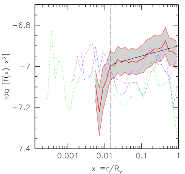
For each cluster we computed the radial profile of $\overline{f}(x)$ versus the distance $x$ from the cluster centre. We then averaged the profiles and fit this to a power-law relation. The result is shown in Fig. 1: the solid line and the surrounding shaded region represent the mean profile with its error.

From the figure we can notice that a single power-law fit as in equation (1) is indeed a good description of the data at most radii. Our best-fitting slope, $\alpha=-1.95$, is slightly steeper than that obtained by Taylor & Navarro (2001). However, at scales corresponding to $\log x\la-1.85$, i.e. for $x\la 0.014$, the mean profile starts showing significant fluctuations from the fit. While a departure from the single power-law is expected for $x\to 0$ (as at small radii the density diverges, but the radial velocity dispersion goes to zero), the observed deviation is probably due to numerical effects.

In order to confirm or dispute this interpretation, we computed the analogous profile for a single cluster, re-simulated with dark matter only, at higher and higher resolution (see Springel et al. 2001a). The resulting profiles are shown in Fig. 1 by the three dotted lines: they correspond to simulations with $6\times 10^{5}$, $3.4\times 10^{6}$ and $1.9\times 10^{7}$ particles inside the virial radius at redshift $z=0$. These profiles, which are plotted from the radius containing 250 particles, are quite noisy because they refer to a single cluster realisation as opposed to our mean curve. However, their slope is quite close to that obtained from our sample, essentially confirming our estimation of $\alpha$. More importantly, the three curves show no systematic deviation from a single power-law at small radii: this seems to confirm the numerical origin of the small scale fluctuations. We therefore decided to consider all the profiles presented in this work only at radii larger than $\log x\la-1.85$. Within this radius our clusters contain on average $\approx 800$ dark matter particles. This is a quite conservative limit, and satisfies the requirements suggested by recent convergence studies (Power et al. 2003).

Notice that the normalisation of the power-law relation for our fit is slightly larger than that resulting from the single high-resolution dark matter-only simulations. This difference could either be due to statistical fluctuations or by the fact that our simulations contain also gas. However, the discrepancy is not really relevant for our model, as in what follows we will only use the slope $\alpha$ of the relation.

3.2 Velocity structure

As a next step we will consider the dark matter velocity dispersion profiles. These are important not only to understand the velocity structure of dark matter haloes, but also to estimate the total cluster mass through the Jeans equation (as done in section 3.4).

In Fig. 2 we show the mean profiles (averaged over our cluster sample) for the radial velocity dispersion $\sigma_{r}(x)$ (top panel), the tangential velocity dispersion $\sigma_{t}(x)$ (central panel) and the velocity anisotropy parameter $\beta(x)\equiv 1-\sigma_{t}^{2}(x)/2\sigma_{r}^{2}(x)$ (bottom panel). The solid bands represent the error on the mean. In order to perform the mean over clusters of different mass, each profile was normalized by the quantity $\sigma_{\rm v}^{2}\equiv GM_{\rm v}/R_{\rm v}$, where $R_{\rm v}$ and $M_{\rm v}$ are the individual virial radii and masses. The vertical dashed line represents the limit of our model, at $\log x=-1.85$. We remind that the velocity anisotropy $\beta$ shows preferred directions in the velocity field. In particular, $\beta=0$ corresponds to an isotropic velocity field, while $\beta<0$ and $0<\beta\leq 1$ indicate predominance of tangential and radial motions, respectively.

Figure 2: Velocity profiles. From top to bottom, different panels refer to radial velocity dispersion $\sigma_{r}(x)$, tangential velocity dispersion $\sigma_{t}(x)$, and velocity anisotropy $\beta(x)$. Velocity dispersions are plotted in units of the virial quantity $\sigma_{\rm v}$. The solid lines and surrounding shaded regions represent the mean profile obtained from our sample of simulated clusters and its error, respectively; dashed lines represent our fitting formulae (equations 2-4; see text for more details). The vertical dashed line is the limit of our model, set at $\log x=-1.85.$

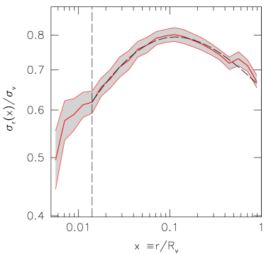
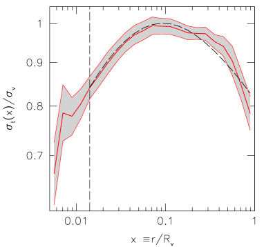
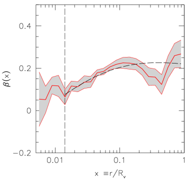
The plots show that in general the dark matter velocity field in clusters is not isothermal nor isotropic. The radial and tangential velocity dispersions decline both at small and large radii, while the radial trend of $\beta$ indicates a predominance of radial motions at large radii, and an almost isotropic velocity field in the inner part, a result consistent with previous studies (e.g. Cole & Lacey 1996; Tormen et al. 1997). We also find that the mean radial velocity (not shown) is still negative at the virial radius, i.e. infall motions are present: this suggests that our clusters are on average not completely relaxed, as clumps of matter are still entering at $z=0$.

Since the three quantities $\sigma_{r}$, $\sigma_{t}$ and $\beta$ are not independent, we can derive any of them using the other two. This should also be true for the analytic fits; therefore we tried fitting each pair of profiles with double power-laws, and derived each third fit by their combination. The solution which best describes the simulated profiles turned out to be fitting the radial velocity dispersion and the velocity anisotropy directly, and getting the tangential velocity dispersion by combination.

The analytical expressions of our fits (hereafter marked by a tilde) are the following:

1. radial velocity dispersion:

   $$\tilde{\sigma}_{r}(x)\equiv\sigma_{r}(x)/\sigma_{\rm v}=\sigma_{r_{0}}x^{0.3}(x+x_{p_{1}})^{-0.48},$$ (2)

   with scale radius $x_{p_{1}}=10^{-1.16}$ and normalization amplitude $\sigma_{r_{0}}=0.67$;

2. velocity anisotropy $\beta(x)$:

   $$\tilde{\beta}(x)=\beta_{0}x^{0.25}(x+x_{p_{2}})^{-0.3},$$ (3)

   with $x_{p_{2}}=10^{-1.1}$ and $\beta_{0}=1.7$;

3. tangential velocity dispersion:

   $$\tilde{\sigma}_{t}(x) \equiv \sigma_{t}(x)/\sigma_{\rm v}$$ (4)

   $$= \tilde{\sigma_{r}}(x)\sqrt{2\left[1-\tilde{\beta}(x)\right]}=\sigma_{r_{0}}x^{0.3}\left(x+x_{p_{1}}\right)^{-0.48}$$

   $$\times \sqrt{2\left[1-\beta_{0}x^{0.25}(x+x_{p_{2}})^{-0.3}\right]}\ .$$

In Fig. 3 we show the mean logarithmic residuals between the actual profiles and our fitting formulae. Error bars represent the error on the mean. Notice that for radial and tangential velocity dispersions the differences are very small and within $1\sigma$ of the mean at most radii. The maximum discrepancies are found at large radii, but they are still below 5 per cent. The velocity anisotropy $\beta(x)$ is equally well fitted at radii $x<0.25$, while differences can be as large as 50 per cent at intermediate distances: $0.3\la x\la 0.5$; this is the range where $\sigma_{t}(x)$ is also showing the largest deviations from our fit. Given the non-trivial shape of the measured velocity anisotropy profile (bottom panel of Fig. 2), we decided not to try a more complicated fit for the sake of simplicity. As we shall see below, the error introduced in the Jeans equation by such deviations is not relevant.

Figure 3: Mean logarithmic residuals between the measured profiles and our fitting formulae (equations 2-4): radial velocity dispersion $\sigma_{r}(x)$ (top panel), tangential velocity dispersion $\sigma_{t}(x)$ (central panel) and velocity anisotropy $\beta(x)$ (bottom panel). Residuals are plotted only for radii larger than the fiducial limit of our fit: $\log x=-1.85$, as set by the analysis of Fig. 1.

3.3 Density structure

The density profile of dark matter haloes has been widely studied in the last few years (e.g. Crone, Evrard & Richstone 1994; Jing et al. 1995; Navarro, Frenk & White 1996, 1997; Tormen, Bouchet & White 1997; Huss, Jain & Steinmetz 1999). There is now a general agreement that a double power-law with a central cusp is a good description of simulated haloes (e.g. NFW), even though the exact value of the inner asymptotic slope is still debated (Moore et al. 1998; Jing & Suto 2000; Jing 2000; Ghigna et al. 2000; Power et al. 2003), possibly due to the presence of systematic and/or numerical effects.

While it is not the purpose of this paper to enter this discussion, we would like to stress that, unlike the majority of previous studies, the dark matter profiles modelled in this work come from simulations where the effect of the hot ICM is properly taken into account: the presence of hot gas, even if not gravitationally dominant, can very well affect also the dark matter structure.

A model for the dark matter density profile is straightforward to obtain using the fitting relations derived in the previous subsections. If we combine the coarse-grained phase-space density profile $\overline{f}(x)$ (equation 1) with the radial velocity dispersion profile $\tilde{\sigma}_{r}(x)$ (equation 2) and solve for the density, we easily get the following approximate fit for the dark matter spatial density distribution:

$$\tilde{\rho}(x)\equiv\frac{\rho(x)}{\rho_{\rm b}}=\frac{\rho_{0}}{x(x+x_{p_{1}})^{1.5}}\ ,$$ (5)

with $\rho_{\rm b}$ the mean background density of the universe; the normalisation factor $\rho_{0}$ is given by

$$\rho_{0}=\frac{(1-f_{\rm b})\Delta_{\rm v}}{6\,\left[(1+2x_{p_{1}})/(1+x_{p_{1}})^{1/2}-2x_{p_{1}}^{1/2}\right]}\ ,$$ (6)

where $\Delta_{\rm v}$ is the virial overdensity specified by the cosmological model; the term $f_{\rm b}=0.097$ is the average baryonic fraction of our cluster sample, measured at the virial radius; it is used to properly weigh the DM component in our simulated clusters.

Notice that for simplicity we have rounded the asymptotic behaviour of this fit to $x^{-1}$ and $x^{-2.5}$ at very small and very large scales, respectively. The exact slopes coming from the combination of the two fitting relations for $\overline{f}(x)$ and $\sigma_{r}(x)$ would be slightly different, $x^{-1.05}$ and $x^{-2.49}$ respectively. However, as we will see, such small differences will not affect our global model.

Figure 4: Mean radial density profile for dark matter: $x^{2}\rho(x)$ (solid line) with error on the mean (shaded region). The dashed and dotted lines refer to our fit (equation 5) and to the NFW fit (equation 7), respectively.

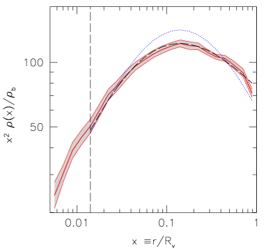
The mean density profile, averaged over the whole sample of simulated clusters, is shown in Fig. 4. As in the previous figures, the shaded region shows the error of the mean, which is relatively small, indicating that the different clusters have quite consistent density profiles. Our model (equation 5) is represented by the dashed line, and agrees very well with the data, always falling inside the error region: only very close to the virial radius there is a small discrepancy. This is a consequence of the sharp change of slope observed in the mean profiles of both $\overline{f}(x)$ and $\sigma_{r}(x)$, and cannot be improved without adding significant complexity to our fitting formulae.

It is interesting to compare our relation to that originally proposed by NFW, which is largely used in the literature to model the halo dark matter distribution. Its expression is the following:

$$\frac{\rho_{\rm NFW}(x)}{\rho_{\rm b}}=\frac{\rho_{0,{\rm NFW}}}{(x/x_{s})(1+x/x_{s})^{2}}\ .$$ (7)

where $x_{s}$ is the scale parameter (inverse of the concentration parameter: $c=1/x_{s}$), and corresponds to our $x_{p}$, while $\rho_{0,{\rm NFW}}$ is the normalisation factor or ‘characteristic density’:

$$\rho_{0,{\rm NFW}}=\frac{(1-f_{\rm b})\Delta_{\rm v}c^{3}}{3[\ln(1+c)-c/(1+c)]}.$$ (8)

Since $\rho_{\rm b}$, $\Delta_{\rm v}$ and $f_{\rm b}$ are specified by the cosmological model, for any given cosmology, $\rho_{0,{\rm NFW}}$ is only a function of $x_{s}$, or of the concentration $c$.

Figure 5: Distribution of the concentration parameter $c$ versus the virial masses $M_{\rm v}$, in units of $h^{-1}M_{\odot}$. Each point refers to a different simulated galaxy cluster.

We found that the value of the NFW concentration parameter which best fits our mean density profile is $c_{\rm NFW}\approx 6.8$. This value is slightly lower than the mean concentration over our cluster sample, which is $\langle c\rangle=7.13$. However, the difference is well within the scatter in the distribution of concentrations, as shown in Fig. 5, where the best fitting concentration for each galaxy cluster is plotted versus the cluster virial mass. The figure also shows that there is no clear systematic trend with mass; consequently it is reasonable to fit the mean profile as representative of the full sample. The resulting NFW profile is shown in Fig. 4 as a dotted line. We notice that for distances $0.04\la x\la 0.4$ the NFW fit overestimates the mean density profiles of the simulations.

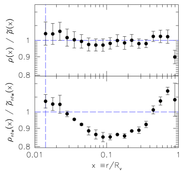
This is more clearly visible in Fig. 6, where we plot the mean logarithmic residuals between the cluster profiles and the analytic fits (equations 5 and 7); error bars indicate the error on the mean. The systematic trend shown by the residuals to the NFW were already noticed in the literature (e.g. Tormen et al. 1997), and indicate that the NFW fit overestimates the actual profiles in the simulations by up to 15 per cent at $x\approx 0.1$, with a rms residual of the mean of 12.1 per cent. This behaviour is strongly reduced if the relation proposed in this paper is used: in this case residuals are always within the error bars, except at distances close to the virial radius, and have a rms of 6.0 per cent. This result is not necessarily at odd with the literature; we wish to remind that the NFW fit was proposed to model the density structure of isolated and relaxed dark matter haloes in dark-matter-only simulations. The fact that our clusters are not all isolated and relaxed, and the presence of a hot gas component, can both play a role in modifying the dark matter profile. We will come back to this issue in the discussion section.

Figure 6: Mean logarithmic residuals between the measured density profiles and the two fitting relations. Top and bottom panels refer to equations (5) and (7), respectively. Error bars represent the error on the mean.

3.4 Mass Estimates

Given the previous relations, the cluster mass inside any given radius can be obtained either by direct integration of the density profile, or by applying the Jeans equation to the system.

Integration of the density profile (equation 5) gives immediately

$$\tilde{M}(x)\equiv\frac{M(<x)}{M_{\rm v}}=\frac{6\rho_{0}}{\Delta_{\rm v}}\left[\frac{x+2x_{p}}{(x+x_{p})^{1/2}}-2x_{p}^{1/2}\right]\ .$$ (9)

The corresponding gravitational potential profile has also an analytic expression:

$$\tilde{\Phi}(x)=-16\pi G\rho_{0}\left[\frac{(x+x_{p})^{1/2}-x^{1/2}}{x}\right].$$ (10)

For comparison, we also report the corresponding relations obtained by integrating the NFW profile (equation 7):

$$\frac{M_{\rm NFW}(<x)}{M_{\rm v}}=(1-f_{\rm b})\frac{\ln(1+cx)-cx/(1+cx)}{\ln(1+c)-c/(1+c)}\$$ (11)

for the mass, and

$$\Phi_{\rm NFW}(x)=-\frac{4\pi G\rho_{\rm 0,{\rm NFW}}}{xc^{3}}\ln\left(1+cx\right),$$ (12)

for the gravitational potential.

However, it is more interesting and useful to estimate the mass profile through the Jeans equation which, for a spherical static system, can be expressed as the ratio between the estimated and true mass:

$$M^{E}(<x)=-\frac{xR_{\rm v}\sigma_{r}^{2}(x)}{G}\left[\frac{d\ln\rho(x)}{d\ln x}+\frac{d\ln\sigma_{r}(x)}{d\ln x}+2\beta(x)\right].$$ (13)

Tormen et al. (1997) and Thomas et al. (1998) have shown that cluster-sized dark matter haloes are indeed reasonably modelled by this equation. Observed galaxy clusters have also been described by such an equation (e.g. the CNOC cluster survey, Carlberg et al. 1997) with results in agreement with those coming from simulations. We stress that we are not imposing the Jeans equation as a constraint to our model: we are using it to test the self-consistency of our density and velocity fitting formulae, assuming that the galaxy clusters obey it. Using the Jeans estimate allows in principle to also weigh the different contributions to the total estimate, and to measure the errors made when one or more terms in the equation are ignored for lack of information on the system.

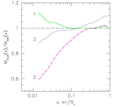
The performance of the different mass estimators is shown in Fig. 7, where we plot the ratio between the actual mass profile (i.e. the mean mass profile of our simulated clusters) and the mass profile obtained by either integrating the density profile or by inserting the analytic fits into the Jeans equation (13). The profiles from simulations were multiplied by a factor $(1+\epsilon^{2}/x^{2})^{3/2}$, where $\epsilon$ is the Plummer equivalent of the actual spline softening, to deconvolve the effect of gravitational softening and thus provide a more accurate comparison at small radii. Curves labeled 1 and 2 refer to estimates based on the integrals of the density models, $\tilde{M}(x)$ (equation 9) and $M_{\rm NFW}(<x)$ (equation 11), respectively; curve 3 refers to the mass obtained from the Jeans equation (13) using the density and velocity profiles given in equations  (2), (3) and (5).

Notice a very good agreement between the actual mass and that derived by integrating our density profile (equation  5). The maximum discrepancy is found at small radii ($\log x\approx-1.85$) and is of the order of 10 per cent. The analogous estimate from the NFW density profiles shows larger discrepancies: roughly 40 per cent at $\log x\approx-1.85$ and 10 per cent at $\log x\approx-1$. On the other hand, both models accurately reproduce the mass profile close to the virial radius, where the errors are of the order of 1-2 per cent.

The mass estimate obtained by the Jeans equation (curve 3) is also very good; its error is always smaller than 10 per cent, suggesting that the model we are proposing is indeed dynamically self-consistent. The main discrepancy is found at distances close to the virial radius; we have checked that this error originates mainly from the incorrect slope of our density profile close to $R_{\rm v}$.

Figure 7: Ratio between the true mass $M_{\rm true}(<x)$ and the one derived from different estimators. Different curves refer to $\tilde{M}(x)$ (equation 9; solid curve 1), $M_{\rm NFW}(<x)$ (equation 11; dashed curve 2); and $M^{E}(<x)$ (equation 13; dotted line 3).

4 Modelling Gas Profiles

4.1 Density structure

In analogy to what has been done in the previous section for the dark matter profiles, in this section we will apply a similar analysis to the radial profiles of the hot gas component. Let us start from the density. Fig. 8 compares the profiles of gas and dark matter, normalised so that they match at the virial radius. The plot shows that the profiles are similar roughly for $x\ga 0.06$, while the gas profile becomes flatter in the internal region. The different internal slope of the two profiles agrees with previous analyses, coming from simulations at smaller resolution (e.g. Navarro, Frenk & White 1995; Eke, Navarro & Frenk 1998; Frenk et al. 1999; Pearce et al. 2000; Lewis et al. 2000; Yoshikawa, Jing & Suto 2000). Recent analytical models of the ICM in galaxy clusters (Komatsu & Seljak 2001) also propose a gas density profile with a flatter inner part. In our case, however, the similarity extends to inner radii than previously found.

Figure 8: Dark matter (dashed curve) and gas (solid curve) density radial profiles. The two curves are normalized to have the same value at the virial radius. The vertical line represents the limit we assumed for our model, at $\log x=-1.85$.

The similarity of the DM and gas profiles in the outer part of the cluster suggested us a first naive approach: that of fitting the gas density profile with the same functional form used for the dark matter, with a different concentration value, assuming of course a different normalization based on the average baryon fraction. The best-fitting NFW profile for the mean gas density turned out to have a concentration $c=4.3$. However, the discrepancy (not shown) between this model and the mean profile in the simulations resulted quite large, the fit having too steep a slope in the inner part, where the gas profiles becomes flatter than $x^{-1}$.

We therefore relaxed the constraint on the inner slope, and tried to fit the gas density profile with a double power-law having the same outer slope as the DM profile, but a different asymptotic behaviour at small radii. The best fitting result turned out to be the following analytic expression:

$$\tilde{\rho}(x)\equiv\frac{\rho(x)}{\rho_{\rm b}}=\frac{\rho_{0}}{(x+x_{p})^{2.5}},$$ (14)

where $x_{p}=0.04$; the normalisation $\rho_{0}$ is given by

$$\rho_{0}=\frac{f_{\rm b}\Delta_{\rm v}}{3}\left[\frac{16x_{p}^{3}/3+40x_{p}^{2}/3+10x_{p}+2}{(x_{p}+1)^{2.5}}-\frac{16x_{p}^{1/2}}{3}\right]^{-1}.$$ (15)

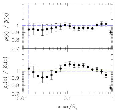
This fit tends to a constant value in the limit $x\to 0$ and decreases as $\rho(x)\propto x^{-2.5}$ at large radii. The upper panel of Fig. 9 compares the proposed fit (dashed curve) to the average profile for the gas density obtained from our simulated clusters (solid curve): the agreement is always very good and the fitting relation falls well inside the shaded region, which displays the 1-$\sigma$ error of the mean. Notice that the results for our simulated clusters are shown starting from the distance containing at least 250 gas particles, while the fitting relations are computing for $\log x>-1.85$, only.

Figure 9: Gas density profile. Top panel: average radial profile $\rho x^{2}$ (solid curve) and its error (shaded region). The dashed and dotted curves represent our model (equation 14) and a $\beta$-model (equation 16), respectively. The vertical line indicates the limit of our fit, taken at $\log x=-1.85$. Bottom panel: logarithmic residuals between the simulated gas density profiles and the analytic models. The upper and lower parts of the plot refer to our model and to the $\beta$-model, respectively. The points and error bars represent the mean ratio and their errors.

A possible different approach is based on the so-called $\beta$-model (Cavaliere & Fusco-Femiano 1976, 1978) which is the density profile most commonly used to describe the gas distribution in observed galaxy clusters. Here the original underlying assumption is that the gas density is proportional to the galaxy density to a given power $\beta$. Since the galaxy distribution was assumed to follow a King profile, the resulting gas density profile is given by

$$\rho_{\beta}(x)=\frac{\rho_{0\beta}}{\left(x^{2}+x_{c}^{2}\right)^{3\beta/2}}\ ,$$ (16)

where $x_{c}$ is the core radius (in units of the virial radius) and the external slope is given by $3\beta$. However, more recent analyses have shown that the galaxy distribution traces the total mass distribution, which is well described by a NFW profile (e.g. Carlberg et al. 1997). Moreover, equation (16) cannot fit - at the same time - the central and external parts of the cluster profiles, as traced by SZ and X-ray observations. Finally, previous numerical works have already shown that the $\beta$-model is unfit to describe the results of (lower resolution) hydrodynamical simulations (e.g. Navarro, Frenk & White 1995; Bartelmann & Steinmetz 1996). Still, it is useful to test the $\beta$-profile against the high-resolution simulations presented in this work. We computed the two parameters $x_{c}$ and $\beta$ by best fitting the mean profile of the gas density, and obtained $x_{c}=10^{-1.53}$ and $\beta=0.7$. The corresponding $\beta$-profile is shown as a dotted curve in the upper panel of Fig. 9. It is clear that there is not agreement with the mean result of our simulations, being too flat at large radii. In order to quantify the goodness of fit for the two models, in the lower panel of the same figure we show the logarithmic residuals between the gas density of simulated clusters and our fit (top) or the $\beta$-model (bottom). While in the first case the ratio is very close to unity for $x\la 0.8$, the $\beta$-model has a 10 per cent deviation for $0.1\la x\la 0.3$ and overestimates the density by 25 per cent at the virial radius.

4.2 Velocity structure

We next consider the gas velocity dispersion profiles, normalized by the virial velocity dispersion $\sigma_{\rm v}$ as we did for the dark matter. Results are shown in Fig. 10, where the solid curve and the shaded region represent, as usual, the mean values from the simulations, and the error on the mean. Only for the profile of the velocity anisotropy $\beta(x)$ we make use of the median instead of the average: since $\beta(x)$ usually fluctuates around zero, an average curve would be strongly affected by numerical fluctuations, and would bias the mean curve away from zero.

Figure 10: Radial velocity profiles for the gas: radial velocity dispersion $\sigma_{r}(x)$ and tangential velocity dispersion $\sigma_{t}(x)$ (top and central panels, respectively; the curves are normalized as in Fig. 2) and velocity anisotropy $\beta(x)$ (bottom panel). In the upper and central panels solid lines and shaded regions are the mean values obtained from our sample of simulated clusters and their errors, respectively; only for $\beta$ we prefer to show the median values and its errors. Dashed lines show our fitting formulae (equations 17-19). The vertical dashed line represents the limit of our model, $\log x=-1.85$.

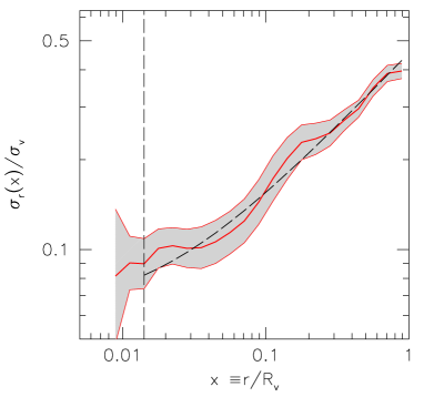
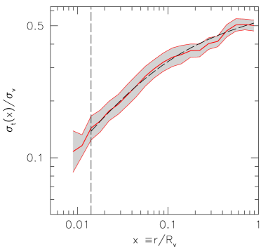
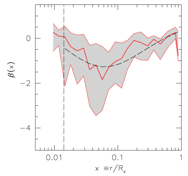
We observed, as expected, that the gas velocity in Fig. 10 behaves very differently from the DM of Fig. 2, due to the different kind of forces acting on the two components. Both the radial and tangential gas velocity dispersions are increasing functions of the distance $x$, even if $\sigma_{r}(x)$ presents a central flattening. The velocity anisotropy $\beta(x)$ is marginally negative in the intermediate part of the clusters ($x\approx 0.1$), denoting a slight predominance of tangential motions. Finally, the gas radial velocity (not shown) is not completely zero, but slightly negative and larger at large radii, suggesting a residual net infall.

Our best analytic fits to the curves for $\sigma_{r}$ and $\sigma_{t}$ are also shown in Fig. 10, indicated by dashed lines; their expressions are:

$$\tilde{\sigma}_{r}(x)\equiv\sigma_{r}(x)/\sigma_{\rm v}=\sigma_{r_{0}}\ (x_{p_{1}}+x)^{0.5}$$ (17)

$$\textrm{where }\sigma_{r_{0}}=0.45\textrm{ and }x_{p_{1}}=10^{-1.72};$$

$$\tilde{\sigma}_{t}(x)\equiv\sigma_{t}(x)/\sigma_{\rm v}=\frac{\sigma_{t_{0}}x^{0.6}}{(x_{p_{2}}+x)^{0.5}}$$ (18)

$$\textrm{where\ }\sigma_{t_{0}}=0.54\textrm{ and }x_{p_{2}}=10^{-1.1}.$$

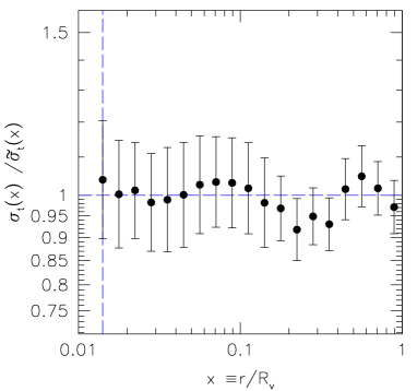
The logarithmic residuals between the mean simulated profiles and our models are plotted in Fig. 11, with mean values and error indicated as usual. The error bars are quite large, showing a large variance in our cluster sample, but the results are always compatible with unity, denoting a good agreement between simulated clusters and models.

Figure 11: Logarithmic residuals between the simulated gas velocity profiles and our models (equations 17-18). Radial velocity dispersion $\sigma_{r}(x)$ and tangential velocity dispersion $\sigma_{t}(x)$ are shown in the upper and bottom panels, respectively. The points and error bars represent the mean ratios and the errors on the mean. The vertical dashed line represents the limit of our model, $\log x=-1.85$.

In order to write a model for the velocity anisotropy $\beta(x)$ we decided to simply combine the two previous fits for the velocity dispersions $\tilde{\sigma}_{t}(x)$ and $\tilde{\sigma}_{r}(x)$:

$$\ \tilde{\beta}(x)\equiv 1-\frac{\tilde{\sigma}_{t}^{2}(x)}{2\tilde{\sigma}_{r}^{2}(x)}=1-\frac{\sigma^{2}_{t_{0}}x^{1.2}}{2\sigma^{2}_{r_{0}}(x_{p_{1}}+x)(x_{p_{2}}+x)}$$ (19)

The resulting curve, displayed as dashed line in the corresponding panel of Fig. 10, well reproduces the behaviour on the median value, showing the self-consistency of our relations.

4.3 Temperature structure

The radial temperature profiles of galaxy clusters, as estimated from X-ray observations, still show large uncertainties. Only recently, thanks to spectroscopic data coming from the Beppo-SAX and Chandra satellites (see, e.g., Allen, Schmidt & Fabian 2001; De Grandi & Molendi 2002; Ettori, De Grandi & Molendi 2002a; Ettori et al. 2002b; Johnstone et al. 2002), the complexity of the thermal structure inside galaxy clusters has been revealed. In particular, observations suggest the presence of a central isothermal region followed by a smooth decline towards the centre. In order to reproduce this feature, different recipes based on the inclusion of radiative cooling and feedback heating have been unsuccessfully attempted in numerical simulations (Lewis et al. 2000; Loken et al. 2002; Muanwong et al. 2002; Valdarnini 2003; Tornatore et al. 2003; Borgani et al. 2004). We remind that these processes are not considered in our non-radiative hydrodynamical simulations; however, they influence only the very central part of galaxy clusters, and so in practice they do not affect the model we propose here. The behaviour of the temperature profile is also observationally not well determined at large radii and shows large variation from object to object. However, there are strong indications that the value of the temperature at the virial radius is approximately a factor of 2 smaller than at the centre. This fact in turn causes errors in the mass estimates obtained using the equation of the hydrostatic equilibrium. Lacking a reliable measure of the radial temperature gradient in clusters based on X-ray observations, it is highly useful to have some indications from numerical simulations. For these reasons we devoted great care in modelling the mean temperature profile.

In the upper panel of Fig. 12 we show the average temperature profile normalized by the estimate of the virial temperature, $T_{\rm v}\equiv(G\mu m_{p}M_{\rm v})/(k_{\rm b}R_{\rm v})$. In this relation $G$ is the gravity constant, $\mu=0.59$ is the mean molecular weight, $m_{p}$ is the proton mass and $k_{\rm b}$ is the Boltzmann constant. The figure clearly shows a nearly isothermal inner region, out to $x\approx 0.2$, with only a hint of positive gradient. At larger radii the temperature starts to decrease, reaching at the virial radius a value about 60 per cent of the central one. The profile we find is in good agreement with previous numerical works (Navarro et al. 1995; Eke et al. 1998; Bryan & Norman 1998; Frenk et al. 1999; Thomas et al. 2001; see, however, Loken et al. 2002; AYMG03) and also with the temperature profile found from the analysis of the Beppo-SAX data by De Grandi & Molendi (2002). However, we remark that the much higher numerical resolution of these simulations makes us more confident in the result and allows us to model the simulated profile with more accuracy.

Figure 12: Gas temperature profile. Top panel: mean radial profile $T(x)$ (normalised to the virial estimate $T_{\rm v}$; solid line) and its error (shaded region). The dashed line refers to our model (equation 20). The vertical line represents the limit of our model, $\log x=-1.85$. Bottom panel: logarithmic residuals between the simulated cluster temperature profile and the analytic model. The points and error bars represent the mean ratio and the errors on the mean, respectively.

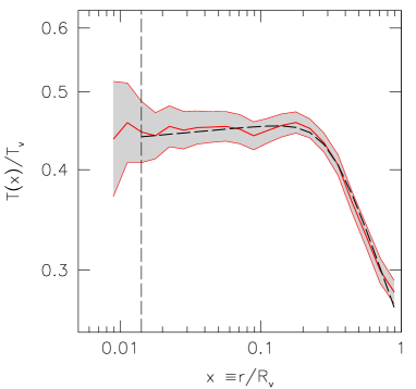
The sudden temperature drop at $x\approx 0.2$ cannot be fit it by a double power-law as those used so far. We model this sharp transition using instead the following expression:

$$\tilde{T}(x)\equiv T(x)/T_{\rm v}=\frac{T_{0}x^{0.016}}{(x^{4}+x_{p}^{4})^{0.13}},$$ (20)

where $T_{0}=0.255$, $x_{p}=10^{-0.51}$; the internal and external logarithmic slopes are approximately $0$ and $-0.5$, respectively. The bottom panel of Fig. 12 shows the logarithmic residuals between the simulated profiles and the previous relation. The mean ratio is very close to unity, with no systematic trend, confirming the accuracy of our fit.

4.4 Mass Estimates

In analogy to the dark matter, we can derive a first estimate of the mass of hot gas inside any given radius by integrating the gas density profile (equation 14). We obtain

$$\tilde{M}_{\rm ICM}(x) \equiv \frac{M_{\rm ICM}(<x)}{M_{\rm v}}=\frac{6\rho_{0}}{\Delta_{\rm v}}$$ (21)

$$\times \left[\frac{8x_{p}^{3}/3+20xx_{p}^{2}/3+5x^{2}x_{p}+x^{3}}{(x_{p}+x)^{2.5}}-\frac{8x_{p}^{1/2}}{3}\right]\ .$$

The short-dashed curve labeled 6 in Fig. 13 is the ratio between the actual gas mass and the mass obtained from equation (21): the agreement between actual and modelled mass profiles is excellent, with differences smaller than 5 per cent at all radii $x>0.02$. The expression in equation (21) will be used below to discuss the baryonic fraction of our clusters.

We now have all the ingredients to discuss other mass estimates using the gas profiles. One of the standard assumption used to derive cluster masses from X-ray data is that the system is in hydrostatic equilibrium: the results of our high-resolution simulations can give us some indications on the accuracy of this assumption, allowing us to evaluate the size of the typical errors made in cluster mass estimation when complete dynamical information are not available.

Assuming a spherical and static gravitational potential, the usual equation for hydrostatic equilibrium can be formally obtained from the Jeans equation (equation 13) by equating the gas internal energy to the dark matter velocity dispersion $\sigma_{r,{\rm DM}}$,

$$\frac{k_{\rm b}T}{\mu m_{p}}=\sigma_{r,{\rm DM}}^{2}$$ (22)

and by assuming an isotropic velocity field: $\beta(x)\equiv 0$. One then obtains the following mass estimate

$$M^{E}(<x)=-\frac{xR_{\rm v}k_{\rm b}T(x)}{G\mu m_{p}}\left[\frac{d\textrm{ln}\rho(x)}{d\textrm{ln}x}+\frac{d\textrm{ln}T(x)}{d\textrm{ln}x}\right].$$ (23)

However, the hypotheses underlying equation (23) are too restrictive for at least two reasons. First, our simulations show that the mean velocity anisotropy $\beta(x)$ is not zero inside the virial radius (see Fig. 10). Second, the replacement of the velocity dispersion with the temperature is not fully justified, due to the residual bulk motions shown in the same figure.

In order to have a more complete description of the gas behaviour, it is more convenient to start directly from the force equation, and to keep all terms coming both from isotropic pressure and from anisotropic velocity dispersion. For a system in a spherical and symmetric potential $\Phi(x)=GM(<x)/x$, this gas dynamical equilibrium equation can be written as:

$$\frac{d\Phi(x)}{dx}=\frac{1}{\rho(x)}\frac{dP(x)}{dx}+\frac{1}{\rho(x)}\frac{d\left[\rho(x)\sigma_{r}^{2}(x)\right]}{dx}+2\beta(x)\frac{\sigma_{r}^{2}(x)}{x}\ .$$ (24)

By substituting the expression for the pressure, $P(x)=\rho(x)k_{\rm b}T(x)/\mu m_{p}$, it is possible to obtain a new mass estimator $M^{E}(<x)\equiv M(<x)/M_{\rm v}$ for the total mass inside $x$ traced by the gas distribution:

$$M^{E}(<x) = -\frac{xR_{\rm v}k_{\rm b}T(x)}{G\mu m_{p}}\left[\frac{d\ln\rho(x)}{d\ln x}+\frac{d\ln T(x)}{d\ln x}\right]-$$ (25)

$$\frac{x\ R_{\rm v}\ \sigma_{r}^{2}(x)}{G}\left[\frac{d\ln\rho(x)}{d\ln x}+\frac{d\ln\sigma_{r}^{2}(x)}{d\ln x}+2\beta(x)\right].$$

We then used this complete equation, together with some simplifications of it, to estimate the cluster mass inside $x$ using the radial profiles we proposed for the various quantities. In particular we considered the following possibilities:

1. a $\beta$-model isothermal sphere, giving:

   $$M^{E}_{1}(<x)=-\frac{xR_{\rm v}k_{\rm b}T(<x)}{G\mu m_{p}}\frac{d\ln\rho_{\beta}(x)}{d\ln x}\ ,$$ (26)

   where $T(<x)$ is the actual mean temperature inside $x$ and $\rho_{\beta}(x)$ is the $\beta$-model defined by equation (16);

2. an isothermal sphere with density profile given by our best fit to the simulations, equation (14), giving:

   $$M^{E}_{2}(<x)=-\frac{xR_{\rm v}k_{\rm b}T(<x)}{G\mu m_{p}}\frac{d\ln\tilde{\rho}(x)}{d\ln x}\ ;$$ (27)

3. the usual hydrostatic equilibrium equation (23) with a $\beta$-model gas density profile (equation 16) and our best fitting relation for the temperature profile (equation 20):

   $$M^{E}_{3}(<x)=-xM_{\rm v}\tilde{T}(x)\left[\frac{d\ln\rho_{\beta}(x)}{d\ln x}+\frac{d\ln\tilde{T}(x)}{d\ln x}\right]\ ;$$ (28)

4. the same equation of hydrostatic equilibrium (23), where the density and temperature profiles are our best fit equations (14) and (20):

   $$M^{E}_{4}(<x)=-xM_{\rm v}\tilde{T}(x)\left[\frac{d\ln\tilde{\rho}(x)}{d\ln x}+\frac{d\ln\tilde{T}(x)}{d\ln x}\right]\ ;$$ (29)

5. the more general model described by equation (25):

   $$M^{E}_{5}(<x) = -xM_{\rm v}\tilde{T}(x)\left[\frac{d\ln\tilde{\rho}(x)}{d\ln x}+\frac{d\ln\tilde{T}(x)}{d\ln x}\right]$$ (30)

   $$+xM_{\rm v}\tilde{\sigma}_{r}^{2}(x)\left[\frac{d\ln\tilde{\rho}(x)}{d\ln x}+\frac{d\ln\tilde{\sigma}_{r}^{2}(x)}{d\ln x}+2\tilde{\beta}(x)\right],$$

   where all the profiles are given by our best fits to the simulations, equations (14), (20), (17) and (19);

Figure 13: Ratio between the true mass $M_{\rm true}$ and the mass derived from different estimators $M_{\rm est}$ presented in the text. The curves refer to $M^{E}_{1}$ (equation 26: dotted line), $M^{E}_{2}$ (equation 27: long-dashed line), $M^{E}_{3}$ (equation 29: short-dashed line), $M^{E}_{4}$ (equation 28: dotted-short-dashed line), $M^{E}_{5}$ (equation 30: solid line). Curve labeled 6 represents the ratio between the actual gas mass and the mass obtained from equation (21); dotted-long-dashed line.

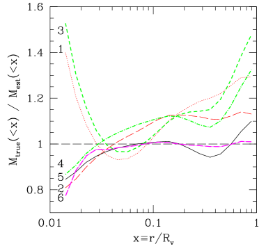
As done for the dark matter component in Fig. 7, we discuss the performance of the different mass estimators by plotting in Fig. 13 the ratio between the true mass profile, i.e. the average mass profile of our simulated clusters, and the previous analytic relations. Curves labeled 1 and 2 refer to estimates based on the isothermal sphere model ($M^{E}_{1}$ using equation 26 and $M^{E}_{2}$ using equation 27); curves labeled 3 and 4 are for a standard hydrostatic equilibrium model using for the temperature the new fit we propose and for the gas density a $\beta$-model ($M^{E}_{3}$, equation 28), or using for temperature and density our new fits ($M^{E}_{4}$, equation 29); curve labeled 5 is for the complete ‘hydrodynamical equilibrium’ model which includes the support from residual gas motions, and uses all the analytical relations we derived ($M^{E}_{5}$, equation 30).

From the figure we notice that the $\beta$-models (curves 1 and 3) underestimate the true cluster mass at most radii, the disagreement being worst at large radii, where the isothermal $\beta$-model (curve 1) is off by up to 30 per cent, and the non-isothermal one (curve 3) is off by up to 50 per cent. This is in agreement with previous results in the literature (see e.g. Muanwong et al. 2002). Using our density profile for the gas (curve 2 and 4) improves the estimate at all radii of interest ($x>0.2$), reducing the mass error at the virial radius to 15 per cent (isothermal model, curve 2) and to roughly 30 per cent (non-isothermal model, curve 4). The complete model (curve 5) is the most accurate at all radii, with an error of 5 to 10 per cent at $x>0.2$. Comparison of curves 4 and 5 shows that the pressure contribution from bulk gas motions is significant at all radii $x>0.1$.

It is also interesting to see that the two isothermal estimators (curves 1 and 2) on average fare better than the non-isothermal ones (curves 3 and 4) at all $x>0.2$. The reason for this counterintuitive result lies in the different temperature used in the isothermal models (average temperature within each radius) compared to the non-isothermal ones (local temperature at each radius). By chance this difference cancels part of the error made by ignoring the gas motion in the outer cluster regions, and effectively makes isothermal estimators more accurate than non-isothermal ones. This is an interesting result: if it were confirmed also when projection effects and observational uncertainties are considered, it could lead to more accurate mass estimations from X-ray observations.

We also note that the incomplete estimators (curves 1 to 4) generally underestimate the actual cluster mass, but a simple isothermal model with the appropriate gas density profile (curve 2) is still accurate to the 15 per cent level.

4.5 Baryonic Fraction

A straightforward consequence of our model is an analytic model for the baryon fraction radial profile, obtained by using the expressions for the dark matter and gas masses (equations 9 and 21):

$$\tilde{f}_{\rm bar}(<x)\equiv\frac{{\tilde{M}}_{\rm gas}(<x)}{\tilde{M}_{\rm gas}(<x)+\tilde{M}_{\rm DM}(<x)}\ .$$ (31)

Notice that $\tilde{f}_{\rm bar}(x<1)\equiv f_{\rm b}=0.097$.

Figure 14: Baryonic fraction. Top panel: radial profile of the baryonic fraction. Solid curve and shaded region indicate the mean and its error for the cluster sample; the dashed curve is the baryonic fraction predicted by integrating the analytic profiles proposed in this paper (equation 31). Bottom panel: logarithmic residuals between the actual and predicted baryonic fractions.

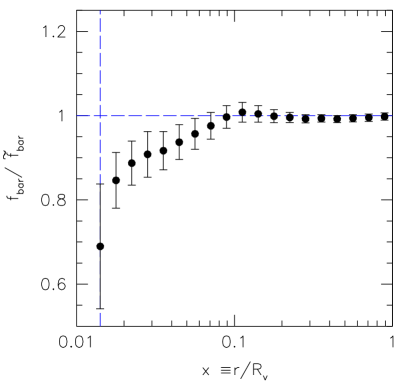
The previous expression is compared to the actual baryon fraction in Fig. 14. The analytic profiles predict a relation (solid curve) that is practically indistinguishable from the actual profile for $x>0.1$, while at smaller radii deviations grows, reaching a 15 per cent overestimate at $x=0.02$. However, this can still be considered an excellent result of our analytic fits.

5 Discussion

5.1 Effect of ICM on the density profile

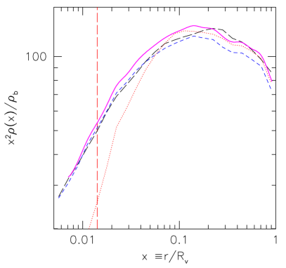
The results of Section 3.3 on dark matter density profiles indicate that the NFW fit has systematic residuals at intermediate radii with respect to the actual mean dark matter profile of our simulated haloes. Although this was already shown by Tormen et al. (1997) on a set of dark matter-only simulations, it is natural to ask more generally whether and how much the presence of a hot gas component affects the dark matter distribution. All the SPH clusters studied in this work were also simulated with dark matter only, using otherwise the same initial conditions and identical parameters for the evolutionary code: we can thus directly compare the density profiles in the two instances.

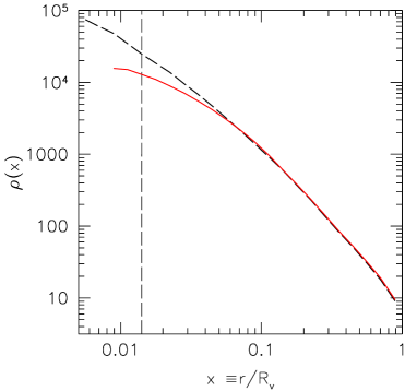
We would like to stress that the NFW profile was originally introduced as a fit for the dark matter profile of isolated and relaxed dark matter haloes in pure N-body simulations, and later it has been used to fit the total profiles of observed clusters. In both cases the fitted profiles represent the total density distribution, not only the dark matter one. Therefore, we think it is here more appropriate to compare the dark matter-only profiles of pure N-body clusters to the total (i.e. dark matter plus hot gas) profiles of our SPH clusters. These are shown in Fig. 15: the short- and long-dashed curves represent the mean dark matter profiles in the SPH runs and in the pure N-body companion runs, respectively, while the dotted curve is the gas density (offset by a factor $f_{\rm b}^{-1}$ for clarity), and the solid curve is the sum of dark matter and gas profiles in the SPH runs. Comparison of the two total profiles (long-dashed and solid curves) shows that the effect of gas is to slightly concentrate the total distribution. An NFW fit on the long-dashed curve (total N-body density) gives a mean concentration $c_{\rm DM}\approx 6.0$, while a fit on the solid curve (total SPH density) gives a concentration $c_{\rm SPH}\approx 6.5$. Thus the effect of adding a hot gas component shifts concentrations up by roughly 10 per cent, an amount comparable to the baryonic fraction of our SPH runs.

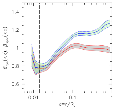
The explanation of this result might be found in the different energy content of DM and gas. As first pointed out by Navarro, Frenk & White (1995), during the accretion of matter onto a cluster, the collisional nature of the ICM delays the gas infall compared to the dark matter. Due to this spatial lag, the gas feels a slightly stronger gravitational field and so acquires extra energy at the expenses of the dark component. This fact was explicitly demonstrated by Pearce, Thomas & Couchman (1994) and by Navarro et al. (1995), but can be also observed by comparing the energy content of the two species through the ratio

$$\beta_{\rm dyn}\equiv\frac{\sigma_{\rm DM}^{2}}{k_{\rm b}T/\mu m_{p}+\sigma_{\rm gas}^{2}}$$ (32)

where $\sigma_{\rm DM}$ and $\sigma_{\rm gas}$ are the one-dimensional velocity dispersions for the dark matter and gas, respectively, and $T$ is the gas temperature. This parameter differs from the usual $\beta_{\rm spec}$ for the extra term $\sigma_{\rm gas}^{2}$, which accounts for the gas bulk energy. In Fig. 16 we show the radial profiles of the average value of $\beta_{\rm dyn}$ in spheres of given radius, $\beta_{\rm dyn}(<x)$. Solid curve and band indicate mean over the cluster sample and its error. This quantity illustrates the energy ratio of dark matter and gas inside a sphere of any radius $x$. It clearly shows that, at radii larger than about $x=0.1$, there is energy equipartition between the two species. Instead, at smaller radii, the gas has a larger energy content than its collisionless companion. The same radius is also close to where the similarity of the gas and dark matter density profiles breaks down, as shown in Fig. 8: the extra energy acquired by the gas makes it further expand, resulting in a flatter profile than that of the DM. For reference, the curve with hatched band is the profile of $\beta_{\rm spec}(<x)$, and shows that neglecting the gas bulk energy hides the existing energy equipartition at large radii.

The result of Fig. 15 seems to indicate that the energy lost by the dark matter allows the halo to further compress and concentrate compared to a pure collisionless collapse. We may speculate that, even if not large per se, this effect could lead to observable differences in the properties of galaxy clusters at small scales, e.g. with respect to gravitational lensing effects.

How well are these profiles fitted by the NFW formula? The rms residual of the mean profile for the pure N-body simulations is 16.7 per cent, comparable to previous findings (e.g. Tormen et al. 1997); the residuals of the mean DM profile in SPH runs is 12.1 per cent; the residual on the total (DM plus ICM) mean profile in the SPH runs is 13.3 per cent: therefore, besides changing the concentration, adding the hot gas component slightly improves the NFW fit compared to the pure N-body runs. This seems to indicate that the departures of the DM density from an NFW model are not due to the addition of gas (which in fact slightly improves the fit), but rather to the fact that our clusters were chosen with no specific criterion on their dynamical status: they are not particularly relaxed, nor necessarily isolated. Just for reference, if we try to fit the same profiles with our relation for the dark matter (equation 5) we obtain the following rms residuals of the mean curve: 9.4 per cent, 6.0 per cent and 4.6 per cent for DM in N-body runs, DM in SPH runs and total density in SPH runs, respectively. Therefore, the fit (equation 5) constitutes an improvement over the NFW in all cases.

Figure 15: Comparison of density profiles in different simulations. The long-dashed curve is the average dark matter profile in the pure N-body runs; the short-dashed curve is the average dark matter profile in SPH simulations; the dotted curve is the average gas profile in the SPH simulations, moved up by a factor $f_{\rm b}^{-1}$, for clarity; the solid curve is the total (dark matter plus gas) profile in SPH simulations.

Figure 16: Cumulative profile of $\beta_{\rm dyn}$. The curve and solid band show the mean value (and its error) for equation (32) calculated in spheres of radius $x$. The curve with hatched band refers to $\beta_{\rm spec}$, i.e. it is obtained from the same equation, but neglecting the gas bulk energy.

5.2 Dependence on the dynamical and environmental status

As already said, we selected our sample in a random way, with no constrain on the dynamics or environment of the objects. On the other hand, the NFW model is known to apply better to clusters which are relaxed and virialized. It is therefore important to investigate how the fitting relations we propose in this paper depend on the dynamical and environmental status.

To this aim, we first created a subsample excluding the systems which show at $z=0$ evidences of a major merging event. Following Tormen et al. (1997), we defined as perturbed those clusters for which the total mass, the dark matter velocity dispersion and the gas temperature show a sudden significant increase (say at least 20 percent in mass) between the two last available outputs. We found 5 such objects: excluding them we obtain a subsample of 12 relaxed clusters, for which we computed the average profiles of all relevant quantities. We found that the resulting average profiles are statistically identical to those coming from the full sample; the only exception is the radial velocity, which is much closer to zero at the virial radius for the relaxed sample. This is consistent with the fact that selecting relaxed objects we tend to exclude systems with significant infalling of matter. More importantly for our considerations, we found that all the fitting relations described in the previous sections give again a proper description also for this subsample. In particular, this is true for the dark matter density profile: this lets us conclude that the difference between the NFW and our density profiles seems not to be due to the presence of merging systems in the original sample.

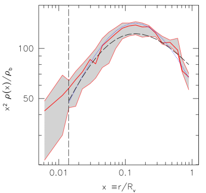
A slightly different approach to select well-behaved objects is considering the environment of each system: following Lanzoni (2000), we defined as isolated those clusters (with virial mass $M_{V}$ and radius $R_{V}$) for which no companion with mass larger than 1/100 $M_{V}$ was found inside a sphere of radius 2 $R_{V}$. In this way we selected, from the original sample of 17, a subset of only 5 isolated clusters (which is also a subset of the 12 relaxed ones). The resulting average profiles are similar to the previous ones, but now the DM density profile (Fig. 17) shows a better agreement with the NFW fit: in particular, the outer slope is somewhat steeper, and the profile at intermediate region is more curved, resulting in a reduction of the residuals.

This fact suggests that the average density DM profile for our sample deviates from the NFW fit mainly because of the inclusion of non-isolated objects.

Figure 17: Dark matter radial density profile for the subsample of 5 isolated clusters. The average and the corresponding error are shown by the solid line and shaded region. Dashed and dotted lines refer to our fit and to the NFW fit, respectively.

5.3 Comparison with Ascasibar et al. (2003)

The recent paper by AYMG03 has presented an analysis similar to ours, applied to a sample of 15 simulated groups and poor clusters. Their approach is different in spirit, as they assume that the gas is in hydrostatic equilibrium and that it follows a polytropic equation of state, whereas we verify our model with the hydrostatic equilibrium equation, and do not assume any equation of state. Nevertheless, we can compare some of their results with ours, once the different definitions of cluster radii are taken into account.

In agreement with AYMG03 we also find that the $\beta$-model is not a good fit to the gas profile of simulated clusters. Instead, we do not agree on the temperature profiles. AYMG03 claim that a central isothermal structure is a numerical artifact of standard SPH schemes which do not implement entropy-conservation, and in fact we used the public version of GADGET, which does not use the entropy-conservation algorithm. However, AYMG03 claim that differences between the two SPH schemes are significant only at scales larger than $\approx 20$ kpc for their Cluster A, and indeed their Fig. 1 indicates that above $\approx 0.03R_{\rm v}$ the gas density and temperature profiles in the two SPH implementations are statistically indistinguishable. On the other hand, our simulations exhibit isothermal cores out to $x\approx 0.2$, a much larger scale. Although we do not have a clear explanation for this discrepancy, it could be that the disagreement is at least enhanced by the different sample used (a sample of rich clusters versus a sample of groups and poor clusters) and by the different dynamical status (if the sample of AYMG03 is less dynamically relaxed than ours, then the central temperature of their systems would be on average perturbed and biased towards higher temperatures). We are currently creating and analysing a sample of clusters at even higher resolution, simulated with the entropy-conserving SPH scheme; the analysis of this new sample should provide a definitive answer to this question.

As a consequence of having an isothermal core, we find that a single polytrope is not a good description of the gas in our clusters. While at radii $x>0.2$ the polytropic index $\gamma$ is close to $1.2$ (the value quoted by AYMG03), at smaller radii $\gamma$ drops to unity. AYMG03 plot their polytropic index only down to $0.2R_{200}$, roughly corresponding to $x=0.15$, so we cannot make a direct comparison at small radii.

6 Conclusions

We have proposed a set of analytical fits which accurately describe the mean radial properties of dark matter and diffuse gas in simulated galaxy clusters. Our relations have been calibrated on a sample of 17 high-resolution SPH clusters, chosen at random from a large parent cosmological simulation. The model provides a self-consistent description of these systems, and can be used to write accurate mass estimates by mean of the Jeans equation for the dark matter distribution and of a similar hydrodynamical equation for the diffuse gas distribution. For dark matter we propose a new model for the density profile, obtained combining phase-space information and radial velocity dispersion; the resulting profile describes our simulations more accurately than the NFW model at $r<0.7R_{\rm v}$. This model differs from the NFW one in that the asymptotic density slope at large radii is $-2.5$ instead of $-3$.

More importantly, we introduce simple new fitting formulae for the DM radial and tangential velocity dispersion profiles and for the velocity anisotropy profile. Radial and tangential velocity dispersions profiles have a maximum value at intermediate radii and decrease both towards the cluster centre and outskirts. Velocity anisotropy is an increasing function of radius: orbits are isotropic in the centre and become increasingly radial orbits at larger radii.

These profiles are tested against the Jeans equation, and are shown to give a self-consistent dynamical model, useful also for mass estimates. We find that the Jeans equation gives a realistic estimate of the mass (with error typically less than 10 per cent). We stress that the focus of our analysis of the dark matter profile is not to propose a replacement for the NFW fit, but to extend the model to all the dark matter profiles relevant for studying the cluster internal structure and dynamics.

We performed a similar study for the gas profiles, introducing new analytic fits for gas density, temperature and velocity dispersions. The average gas density profile of our sample is well described by a double power-law, similar to the dark matter density at $r>0.06R_{\rm v}$, and approaching a constant density towards the centre. The average temperature profile shows an isothermal core extending to $r\approx 0.2R_{\rm v}$, followed by a steep decrease that reaches a factor two lower around the virial radius.

The gas velocity is not zero inside the clusters: residual motions become smaller towards the centre - showing that the infalling gas slows down as it sinks towards the cluster centre - and are isotropic or slightly tangential. Models for the gas velocity profiles are required because the gas on average retains residual motions even inside the virial radius, and this provides non-negligible anisotropic pressure support to the equilibrium of the system. For this reason we generalized the hydrostatic equilibrium equation by adding velocity terms analogous to those used in the Jeans equation for dark matter. This ‘hydrodynamical equilibrium’ equation is in fact a better description of the system and provides a more accurate estimator of the actual mass enclosed by any radius $x$. However, if gas velocity are neglected, a simple isothermal model fares better than a non-isothermal one: if our gas density profile is adopted, then the actual cluster mass is recovered to better than 15 per cent at all radii of interest.

The dark matter and total density profiles in our SPH simulations appear to be more centrally concentrated than those coming from identical - but collisionless - simulations. In terms of NFW halo concentrations, these increase by an amount comparable to the baryonic fraction. Nevertheless, the addition of a hot gas component does not degrade (but even improves) the goodness of fit of a NFW profile. Therefore, the fact that our clusters are better fitted by the profile proposed in equation (5) is not due to the presence of the ICM. On the contrary we showed that it is due to the presence, in our sample, of clusters in various environmental situations, as opposed to having a sample of isolated systems.

The shape of the gas density profile at small radii is at least partially explained by the gas expansion caused by the energy gain from dark matter during the collapse. Proper inclusion of the gas bulk energy shows that the final energy budget is equally shared between the two species at radii $r>0.1R_{\rm v}$, while at smaller radii the gas is hotter than the dark matter. This energy unbalance is probably also the reason of the further global compression of the system compared to a pure collisionless collapse. It would be interesting to investigate whether this effect is large enough to produce observational signatures.

The analytical fits proposed in this work give an overall robust and accurate description of the average dark matter and hot gas properties of galaxy clusters. They have immediate applications in cosmology, as one can derive from them the radial dependence of many observables in the X-ray, SZ and lensing domains.

Work is also in progress to extend this analysis to a sample of cluster simulations where the gas is heated by non-gravitational processes at high redshift, providing better agreement between the X-ray properties of simulated and observed clusters.

References

- [1] Allen S.W., Schmidt R.W., Fabian A.C., 2001, MNRAS, 328, L37
- [2] Ascasibar Y., Yespes G., Mueller V., Gottloeber S., 2003, MNRAS, 346, 731 (AYMG03)
- [3] Barnes J.E., Hut P., 1986, Nat, 324, 446
- [Bartelmann 1998] Bartelmann M., Huss A., Colberg J.M., Jenkins A., Pearce F.R., 1998, A&A, 330, 1
- [4] Bartelmann M., Steinmetz M., 1996, MNRAS, 283, 431
- [5] Bertschinger E., 1985, ApJS, 58, 39
- [6] Borgani S., et al., 2004, MNRAS, in press, astro-ph/0310794
- [7] Bryan G., Norman M.L., 1998, ApJ, 495, 80
- [8] Carlberg R.G., et al., 1997, ApJ, 485, L13
- [9] Cavaliere A., Fusco-Femiano R., 1976, A&A, 49, 137
- [10] Cavaliere A., Fusco-Femiano R., 1978, A&A, 70, 677
- [11] Cole S., Lacey C., 1996, MNRAS, 281, 716
- [Crone 1994] Crone M.M., Evrard A.E., Richstone D.O., 1994, ApJ, 434, 402
- [12] De Grandi S., Molendi S., 2002, ApJ, 567, 1
- [13] Eke V.R., Cole S., Frenk C.S., 1996, MNRAS, 282, 263
- [14] Eke V.R., Navarro J F., Frenk C.S., 1998, ApJ, 503, 569
- [15] Ettori S., De Grandi S., Molendi S., 2002a, A&A, 391, 841
- [16] Ettori S., Fabian A.C., Allen S.W., Johnstone R.M., 2002b, MNRAS, 331, 635
- [17] Frenk C.S., et al., 1999, ApJ, 525, 554
- [Ghigna 2000] Ghigna S., Moore B., Governato F., Lake G., Quinn T., Stadel J., 2000, ApJ, 544, 616
- [Hiotelis 2002] Hiotelis N., 2002a, A&A, 382, 84
- [Hiotelis 2002] Hiotelis N., 2002b, NewA, 7, 531
- [Huss 1999] Huss A., Jain B., Steinmetz M., 1999, ApJ, 517, 64
- [18] Jenkins A., Frenk C.S., White S.D.M., Colberg J.M., Cole S., Evrard A.E., Couchman H.M.P., Yoshida N., 2001, MNRAS, 321, 372
- [19] Jing Y.P., 2000, ApJ, 535, 30
- [Jing 1995] Jing Y.P., Mo H.J., Borner G., Fang L.Z., 1995, MNRAS, 276, 417
- [20] Jing Y.P., Suto Y., 2000, ApJ, 529, L69
- [21] Jing Y.P., Suto Y., 2002, ApJ, 574, 538
- [22] Johnstone R.M., Allen S.W., Fabian A.C., Sanders J.S., 2002, MNRAS, 336, 299
- [Komatsu 2001] Komatsu E., Seljak U., 2001, MNRAS, 327, 1353
- [23] Lanzoni B., 2000, Ph.D. thesis, Universitè de Paris 7
- [24] Lee J., Suto Y., 2003, ApJ, 585, 151
- [25] Lewis G.F., Babul A., Katz N., Quinn T., Hernquist L., Weinberg D.H., 2000, ApJ, 536, 623
- [26] Loken C., Norman M.L., Nelson E., Burns J., Bryan G.L., Motl P., 2002, ApJ, 579, 571
- [Meneghetti 2003] Meneghetti M., Bartelmann M., Moscardini L., 2003, MNRAS, 340, 105
- [27] Moore B., Governato F., Quinn T., Stadel J., Lake G., 1998, ApJ, 499, L5
- [28] Muanwong O., Thomas P.A., Kay S.T., Pearce F.R., 2002, MNRAS, 336, 527
- [29] Navarro J.F., Frenk C.S., White S.D.M., 1995, MNRAS, 275, 720
- [30] Navarro J.F., Frenk C.S., White S D.M., 1996, ApJ, 462, 563
- [Navarro 1997] Navarro J.F., Frenk C.S., White S.D.M., 1997, ApJ, 490, 493 (NFW)
- [31] Pearce F.R., Thomas P.A., Couchman H.M.P., 1994, MNRAS, 268, 953
- [32] Pearce F.R., Thomas P.A., Couchman H.M.P., Edge A.C., 2000, MNRAS, 317, 1029
- [Power 2003] Power C., Navarro J.F., Jenkins A., Frenk C.S., White S.D.M., Springel V., Stadel J., Quinn T., 2003, MNRAS, 338, 14
- [Sheth 2001] Sheth R.K., Hui L., Diaferio A., Scoccimarro R., 2001, MNRAS, 325, 1288
- [33] Springel V., White S.D.M., Tormen G., Kauffmann G., 2001a, MNRAS, 328, 726
- [34] Springel V., Yoshida N., White S.D.M., 2001b, NewA, 6, 79
- [Suto 1998] Suto Y., Sasaki S., Makino N., 1998, ApJ, 509, 544
- [Taylor 2001] Taylor J.E., Navarro J.F., 2001, ApJ, 563, 483
- [35] Thomas P.A., Muanwong O., Pearce F.R., Couchman H.M.P., Edge A.C., Jenkins A., Onuora L., 2001, MNRAS, 324, 450
- [36] Thomas P.A. et al., 1998, MNRAS, 296, 1061
- [37] Tormen G., Bouchet F.R., White S.D.M., 1997, MNRAS, 286, 865
- [38] Tormen G., Moscardini L., Yoshida N., 2004, MNRAS, in press, astro-ph/0304375
- [39] Tornatore L., Borgani S., Springel V., Matteucci F., Menci N., Murante G., 2003, MNRAS, 342, 1025
- [40] Valdarnini R., 2003, MNRAS, 339, 1117
- [41] Yoshida N., Sheth R.K. Diaferio A., 2001, MNRAS, 328, 669
- [42] Yoshikawa K., Jing Y.P., Suto Y., 2000, ApJ, 535, 593