The Skewness of the Aperture Mass Statistic

Abstract

We present simple formulae for calculating the skewness and kurtosis of the aperture mass statistic for weak lensing surveys which is insensitive to masking effects of survey geometry or variable survey depth. The calculations are the higher order analogs of the formula given by Schneider, van Waerbeke & Mellier (2002) which has been used to compute the variance of the aperture mass from several lensing surveys. As our formula requires the three-point shear correlation function, we also present an efficient tree-based algorithm for measuring it. We show how our algorithm would scale in computing time and memory usage for future lensing surveys. We also apply the procedure to our CTIO survey data, originally described in Jarvis et al. (2003). We find that the skewness is positive (inconsistent with zero) at the $2\sigma$ level. However, the signal is too noisy from this data to usefully constrain cosmology.

1 Introduction

One of the most useful statistics for probing the power spectrum with weak gravitational lensing is the aperture mass statistic, $M_{\rm ap}$. The aperture mass was first proposed by Kaiser (1995) and Schneider (1996) for estimating the masses of clusters, and is essentially an estimate of the convergence, $\kappa$, within a circular aperture. The convergence is proportional to the projected mass density relative to the average value in the field, hence the name aperture mass.

Since the aperture mass is relative to the average value, the statistic $\langle\mbox{$M_{\rm ap}$}\rangle$ gives 0 over the whole field. However, higher order moments of the aperture mass are non-zero, and the variance, $\langle M_{\rm ap}^{2}\rangle$, has proved very useful for weak lensing researchers, with many studies to date including this statistic in their analysis (e.g. Hoekstra, Yee & Gladders, 2002; van Waerbeke et al., 2002; Jarvis et al., 2003; Hamana et al., 2003). This statistic is a good probe of the power spectrum, and thus measures the extent of the Gaussian fluctuations of the density of the universe.

However, any non-Gaussian component is not measured by the variance. Further, the density fluctuations must be non-Gaussian, since the density contrast is constrained to be greater than -1, but it can be arbitrarily large in the positive direction. Clusters generally have density contrasts of more than 200. Thus, the density fluctuations, which have a mean of 0 by definition, must be skewed towards positive values. Indeed, this non-Gaussianity has recently been detected in the VIRMOS-DESCART survey by two groups (Bernardeau, Mellier & van Waerbeke, 2002; Pen et al., 2003).

The lowest order measures of the non-Gaussianity using the shear field are called three-point statistics, since they require measurements of three shear values and their relative positions and orientations. Three-point statistics have the potential to be very useful for cosmology, since they can, in combination with two-point statistics, determine $\Omega_{m}$ and $\sigma_{8}$ independently (Bernardeau, van Waerbeke & Mellier, 1997; Jain & Seljak, 1997; Schneider et al., 1998). They can also be used to constrain the properties of halos such as the inner slope and typical concentration parameters (Takada & Jain, 2003). In this paper, we investigate a particular three-point statistic, the skewness of the aperture mass, $\langle M_{\rm ap}^{3}\rangle$.

When Schneider et al. (1998) proposed the use of the aperture mass for cosmic shear measurements, they introduced the form of the statistic which has been used by almost all weak lensing studies to date. However, we find that calculations of the three-point statistic is significantly easier using the form introduced by Crittenden et al. (2002). Namely,

$$\mbox{$M_{\rm ap}$}(R) =\int d^{2}\mn@boldsymbol{r}U_{R}(r)\kappa(\mn@boldsymbol{r})$$ (1)

$$=\int d^{2}\mn@boldsymbol{r}Q_{R}(r)\gamma_{t}(\mn@boldsymbol{r})$$ (2)

$$U_{R}(r) =\frac{1}{2\pi R^{2}}\left(1-\frac{r^{2}}{2R^{2}}\right)\exp\left(-\frac{r^{2}}{2R^{2}}\right)$$ (3)

$$Q_{R}(r) =-U_{R}(r)+\frac{2}{r^{2}}\int_{0}^{r}r^{\prime}dr^{\prime}U_{R}(r^{\prime})$$ (4)

$$=\frac{r^{2}}{4\pi R^{4}}\exp\left(-\frac{r^{2}}{2R^{2}}\right)$$ (5)

where $\kappa$ is the convergence, $\gamma_{t}$ is the tangential component of the shear, and $\mn@boldsymbol{r}$ is measured from the centre of the aperture.

We also note that Zhang et al. (2003) has shown that this form of the aperture mass is more sensitive for constraining $\Omega_{m}$ than other forms.

There are several features of the aperture mass statistic which makes it very useful. First, it probes the power spectrum with a very narrow window function, $W(\eta)$. Schneider et al. (1998) derive the relation:

$$\mbox{$\langle M_{\rm ap}^{2}\rangle$}(R) =\frac{1}{2\pi}\int d^{2}\mn@boldsymbol{k}P(k)W(kR)$$ (6)

$$W(kR) =\tilde{U}_{R}(k)^{2}$$ (7)

$$=\left[\frac{k^{2}R^{2}}{2}\exp\left(-\frac{k^{2}R^{2}}{2}\right)\right]^{2}$$ (8)

$$W(\eta) =\frac{\eta^{4}}{4}\exp(-\eta^{2})$$ (9)

where the tilde ($~{}\tilde{}~{}$) indicates the Fourier transform. This window function $W(\eta)\propto\eta^{4}$ for small $\eta$, and drops super-exponentially for large $\eta$, peaking at $\eta=2$.

Another benefit of the aperture mass is that it has (nearly) finite support in real space, so it is calculable. The ideal window function would be a delta function, $W(\eta)=\delta_{D}(\eta-\eta_{0})$, so the statistic would directly probe $P(\eta_{0}/R)$. However, to have infinitesimal extent in k-space would require infinite extent in real space, and thus be incalculable. $\langle M_{\rm ap}^{2}\rangle$ thus has the advantage that it is compact in real space as well.

The third benefit is that it measures purely the so-called E-mode of the shear field. There is a corresponding statistic, $M_{\times}$, which measures the B-mode:

$$\mbox{$M_{\times}$}(R)=\int d^{2}\mn@boldsymbol{r}Q_{R}(x)\gamma_{\times}(\mn@boldsymbol{r}),$$ (10)

where the cross-component of the shear, $\gamma_{\times}$, is oriented at an angle of $45$ degrees relative to $\gamma_{t}$. Then the variance of this measure, $\langle M_{\times}^{2}\rangle$  is a measure of the B-mode power in the shear field, which is generally taken to be a measure of the contamination from residual systematics, such as uncorrected effects of the point-spread functions. Intrinsic alignments (Crittenden et al., 2002) and source clustering (Schneider et al., 2002) can also produce B-mode signal, but the level of both of these is generall expected to be very low for scales larger than $1\arcmin$.

The only problem with calculating these statistics directly is that real lensing surveys have regions which are masked out due to survey geometry, bright stars, bad seeing, etc. Thus the aperture mass statistic runs the risk of losing azimuthal symmetry due to the masking. Since the statistic depends on azimuthal symmetry for the angular integrals, a direct calculation of $\langle M_{\rm ap}^{2}\rangle$ and $\langle M_{\times}^{2}\rangle$ will leak some of the E and B-mode power into the other statistic. This may only be of order a 10 per cent effect or less for typical surveys, but with the goal of precision cosmology, another method of calculation is typically used, first derived by Crittenden et al. (2002) and then refined by Schneider et al. (2002).

They have shown that the aperture mass variance can be calculated from an integral of the correlation functions in an equation of the form:

$$\mbox{$\langle M_{\rm ap}^{2}\rangle$}(R) =\frac{1}{2}\int\frac{sds}{R^{2}}\left[\xi_{+}(s)T_{+}\left(\frac{s}{R}\right)+\xi_{-}(s)T_{-}\left(\frac{s}{R}\right)\right]$$ (11)

$$\mbox{$\langle M_{\times}^{2}\rangle$}(R) =\frac{1}{2}\int\frac{sds}{R^{2}}\left[\xi_{+}(s)T_{+}\left(\frac{s}{R}\right)-\xi_{-}(s)T_{-}\left(\frac{s}{R}\right)\right]$$ (12)

where $\xi_{+,-}$ are the two-point shear correlation functions (defined more precisely in §2) and $T_{+,-}$ are known functions (also defined in §2).

The third moment of the aperture mass, $\langle M_{\rm ap}^{3}\rangle$ was originally suggested by Schneider et al. (1998) as a statistic for investigating the non-Gaussianity of the shear field. It is useful as a cosmological probe, since (as these authors showed) its dependence on $\Omega_{m}$ and $\sigma_{8}$ are somewhat orthogonal to that of $\langle M_{\rm ap}^{2}\rangle$, so the combination of the two statistics can be used to determine $\Omega_{m}$ and $\sigma_{8}$ separately. In particular $\mbox{$\langle M_{\rm ap}^{3}\rangle$}/\mbox{$\langle M_{\rm ap}^{2}\rangle$}^{2}$ scales approximately as $1/\Omega_{m}$, independent of $\sigma_{8}$.

However, a direct measurement of $\langle M_{\rm ap}^{3}\rangle$ using apertures would be even more affected by masking than the variance is. Thus, in this paper, we derive formulae similar to Equations (11,12) for $\langle M_{\rm ap}^{3}\rangle$ and $\langle M_{\times}^{3}\rangle$  in terms of the three-point correlation function.

The signal-to-noise (S/N) for $\langle M_{\rm ap}^{3}\rangle$ is significantly lower than for $\langle M_{\rm ap}^{2}\rangle$. As we will show below, our total S/N for $\langle M_{\rm ap}^{3}\rangle$ is of order unity for the roughly $10^{6}$ galaxies in our CTIO survey, compared to a S/N of about 7 for $\langle M_{\rm ap}^{2}\rangle$ (Jarvis et al., 2003). As the S/N scales as $N_{\rm gal}^{1/2}$, we would need about $10^{8}$ galaxies to make a good measurement of $\langle M_{\rm ap}^{3}\rangle$. Planned surveys such as those from the Supernova Anisotropy Probe (SNAP) and the Large-aperture Synoptic Survey Telescope (LSST) will do just that. Actually, the S/N also increases when one goes deeper, which both of these telescopes will do, so their S/N should be somewhat better than 10. In any case, the large number of galaxies from these future missions demands efficient algorithms for calculating $\langle M_{\rm ap}^{3}\rangle$, such as the one presented herein.

In §2, we define our notations and briefly rederive the above equations (11,12) in a manner that will lend itself to generalization to the three-point version. This is important, since we found that the derivations given by Crittenden et al. (2002) and Schneider et al. (2002) do not generalize easily to the three-point case. The method is fairly similar to that of Pen et al. (2003), although they use a tensor formulation, which is a bit unwieldy, having 64 components for the three-point correlation function (8 of which are unique). Then §3 will derive the corresponding equations for the three-point statistic. §4 describes our algorithm for calculating the three-point correlation function. In §5, we then apply the formulae to simulated data to check their validity, and also to our CTIO survey data.

2 Variance of the Aperture Mass

We follow the notation of Schneider et al. (2002) to describe the E and B-mode components of the shear field by defining the lensing potential, $\psi$, to be complex.

$$\psi=\psi^{E}+i\psi^{B}$$ (13)

The convergence, $\kappa$, and shear, $\gamma$, are related to the potential by

$$\kappa =\frac{1}{2}\nabla^{2}\psi$$ (14)

$$\gamma =\frac{1}{2}\left(\frac{\partial}{\partial x}+i\frac{\partial}{\partial y}\right)^{2}\psi$$ (15)

Since the convergence is the projected matter density, it is real for pure lensing fields. Thus, lensing produces only E-mode fields, and the B-mode is generally used to check for residual systematics or the aforementioned effects of intrinsic alignments or sourse clustering.

With a complex $\kappa$, Equation (1) would give us a complex value for $M_{\rm ap}$. However, using Equation (10), and defining $M=\mbox{$M_{\rm ap}$}+i\mbox{$M_{\times}$}$, we find

$$M(R) =\int d^{2}\mn@boldsymbol{r}U_{R}(r)\kappa(\mn@boldsymbol{r})$$ (16)

$$=-\int d^{2}\mn@boldsymbol{r}Q_{R}(r)\gamma(\mn@boldsymbol{r})e^{-2i\phi}$$ (17)

where $\phi$ is the polar angle of $\mn@boldsymbol{r}$.

Using this definition, the expectation value of $M^{2}$ is

$$\mbox{$\langle M^{2}\rangle$}(R)=\int d^{2}\mn@boldsymbol{r}_{1}\int d^{2}\mn@boldsymbol{r}_{2}Q_{R}(r_{1})Q_{R}(r_{2})\langle\gamma(\mn@boldsymbol{r}_{1})\gamma(\mn@boldsymbol{r}_{2})\rangle e^{-2i(\phi_{1}+\phi_{2})}$$ (18)

We now define the ‘natural components’ of the two-point shear correlation function as:

$$\xi_{-}(s) =\langle\gamma(\mn@boldsymbol{r})\gamma(\mn@boldsymbol{r}+\mn@boldsymbol{s})e^{-4i\alpha}\rangle$$ (19)

$$\xi_{+}(s) =\langle\gamma(\mn@boldsymbol{r})\gamma^{*}(\mn@boldsymbol{r}+\mn@boldsymbol{s})\rangle$$ (20)

where $\alpha$ is the polar angle of $\mn@boldsymbol{s}$.

Then, Equation (18) becomes (taking $\mn@boldsymbol{r}_{2}=\mn@boldsymbol{r}_{1}+\mn@boldsymbol{s}$, and dropping the subscript for $\mn@boldsymbol{r}_{1}$)

$$\mbox{$\langle M^{2}\rangle$}(R)=\int d^{2}\mn@boldsymbol{r}\int d^{2}\mn@boldsymbol{s}Q_{R}(r)Q_{R}(|\mn@boldsymbol{r}+\mn@boldsymbol{s}|)\xi_{-}(s)e^{2i(2\alpha-\phi_{1}-\phi_{2})}$$ (21)

To evaluate this, we treat $\mn@boldsymbol{r}$ and $\mn@boldsymbol{s}$ as complex numbers, so $\mn@boldsymbol{s}=s\exp(i\alpha)$, $\mn@boldsymbol{r}=r\exp(i\phi_{1})$, and $\mn@boldsymbol{r}+\mn@boldsymbol{s}=|\mn@boldsymbol{r}+\mn@boldsymbol{s}|\exp(i\phi_{2})$. Then

$$\mbox{$\langle M^{2}\rangle$}(R) =\int d^{2}\mn@boldsymbol{s}\xi_{-}(s)\frac{\mn@boldsymbol{s}^{4}}{s^{4}}\int d^{2}\mn@boldsymbol{r}Q_{R}(r_{1})Q_{R}(|\mn@boldsymbol{r}+\mn@boldsymbol{s}|)\frac{(\mn@boldsymbol{r}^{*}+\mn@boldsymbol{s}^{*})^{2}}{|\mn@boldsymbol{r}+\mn@boldsymbol{s}|^{2}}\frac{\mn@boldsymbol{r}^{*2}}{r^{2}}$$ (22)

$$=\int\frac{sds}{R^{2}}\xi_{-}(s)\left[\frac{s^{4}}{128R^{4}}\exp\left(-\frac{s^{2}}{4R^{2}}\right)\right]$$ (23)

$$\equiv\int\frac{sds}{R^{2}}\xi_{-}(s)T_{-}\left(\frac{s}{R}\right)$$ (24)

where ^∗ indicates complex conjugate. (The evaluation of the integral in Equation (22) is straightforward in Cartesian coordinates, where each complex value is represented as, for example, $\mn@boldsymbol{r}=x+iy$.)

A similar procedure can be used to evaluate $\langle MM^{*}\rangle$:

$$\mbox{$\langle MM^{*}\rangle$}(R) =\int d^{2}\mn@boldsymbol{r}\int d^{2}\mn@boldsymbol{s}Q_{R}(r)Q_{R}(|\mn@boldsymbol{r}+\mn@boldsymbol{s}|)\langle\gamma(\mn@boldsymbol{r})\gamma^{*}(\mn@boldsymbol{r}+\mn@boldsymbol{s})\rangle e^{-2i(\phi_{1}-\phi_{2})}$$ (25)

$$=\int d^{2}\mn@boldsymbol{s}\xi_{+}(s)\int d^{2}\mn@boldsymbol{r}Q_{R}(r)Q_{R}(|\mn@boldsymbol{r}+\mn@boldsymbol{s}|)\frac{(\mn@boldsymbol{r}+\mn@boldsymbol{s})^{2}}{|\mn@boldsymbol{r}+\mn@boldsymbol{s}|^{2}}\frac{\mn@boldsymbol{r}^{*2}}{r^{2}}$$ (26)

$$=\int\frac{sds}{R^{2}}\xi_{+}(s)\left[\frac{s^{4}-16R^{2}s^{2}+32R^{4}}{128R^{4}}\exp\left(-\frac{s^{2}}{4R^{2}}\right)\right]$$ (27)

$$\equiv\int\frac{sds}{R^{2}}\xi_{+}(s)T_{+}\left(\frac{s}{R}\right)$$ (28)

Finally we can convert these expressions into formulae for $\langle M_{\rm ap}^{2}\rangle$ and $\langle M_{\times}^{2}\rangle$ individually through the expressions:

$$\mbox{$\langle M_{\rm ap}^{2}\rangle$}+i\mbox{$\langle M_{\rm ap}M_{\times}\rangle$} =\frac{1}{2}\left(\mbox{$\langle MM^{*}\rangle$}+\mbox{$\langle M^{2}\rangle$}\right)$$ (29)

$$\mbox{$\langle M_{\times}^{2}\rangle$}-i\mbox{$\langle M_{\rm ap}M_{\times}\rangle$} =\frac{1}{2}\left(\mbox{$\langle MM^{*}\rangle$}-\mbox{$\langle M^{2}\rangle$}\right)$$ (30)

So,

$$\mbox{$\langle M_{\rm ap}^{2}\rangle$}(R)+i\mbox{$\langle M_{\rm ap}M_{\times}\rangle$}(R) =\frac{1}{2}\int sds\left[\xi_{+}(s)T_{+}\left(\frac{s}{R}\right)+\xi_{-}(s)T_{-}\left(\frac{s}{R}\right)\right]$$ (31)

$$\mbox{$\langle M_{\times}^{2}\rangle$}(R)-i\mbox{$\langle M_{\rm ap}M_{\times}\rangle$}(R) =\frac{1}{2}\int sds\left[\xi_{+}(s)T_{+}\left(\frac{s}{R}\right)-\xi_{-}(s)T_{-}\left(\frac{s}{R}\right)\right]$$ (32)

where

$$T_{+}(x) =\frac{x^{4}-16x^{2}+32}{128}\exp\left(-\frac{x^{2}}{4}\right)$$ (33)

$$T_{-}(x) =\frac{x^{4}}{128}\exp\left(-\frac{x^{2}}{4}\right)$$ (34)

This result agrees with that obtained from the formulae in Schneider et al. (2002) as well as the formulae in Crittenden et al. (2002). Also, Pen et al. (2003) gives a formula for a tensor form of Equations 31 and 32, which can be expanded to agree with our results.

3 Third Moment of the Aperture Mass

We now follow the same procedure as in §2 for evaluating $\langle M^{3}\rangle$ and $\langle M^{2}M^{*}\rangle$.

$$\mbox{$\langle M^{3}\rangle$}(R)=-\int d^{2}\mn@boldsymbol{r}\int d^{2}\mn@boldsymbol{s}\int d^{2}\mn@boldsymbol{t}Q_{R}(r)Q_{R}(|\mn@boldsymbol{r}+\mn@boldsymbol{s}|)Q_{R}(|\mn@boldsymbol{r}+\mn@boldsymbol{t}|)\langle\gamma(\mn@boldsymbol{r})\gamma(\mn@boldsymbol{r}+\mn@boldsymbol{s})\gamma(\mn@boldsymbol{r}+\mn@boldsymbol{t})\rangle e^{-2i(\phi_{1}+\phi_{2}+\phi_{3})}$$ (35)

For the ‘natural components’ of the three-point correlation function, we follow Schneider & Lombardi (2002) and define:

$$\Gamma_{0}(s,\mn@boldsymbol{t}^{\prime}) =\langle\gamma(\mn@boldsymbol{r})\gamma(\mn@boldsymbol{r}+\mn@boldsymbol{s})\gamma(\mn@boldsymbol{r}+\mn@boldsymbol{t})e^{-2i(\alpha_{1}+\alpha_{2}+\alpha_{3})}\rangle$$ (36)

$$\Gamma_{1}(s,\mn@boldsymbol{t}^{\prime}) =\langle\gamma^{*}(\mn@boldsymbol{r})\gamma(\mn@boldsymbol{r}+\mn@boldsymbol{s})\gamma(\mn@boldsymbol{r}+\mn@boldsymbol{t})e^{-2i(-\alpha_{1}+\alpha_{2}+\alpha_{3})}\rangle$$ (37)

$$\Gamma_{2}(s,\mn@boldsymbol{t}^{\prime}) =\langle\gamma(\mn@boldsymbol{r})\gamma^{*}(\mn@boldsymbol{r}+\mn@boldsymbol{s})\gamma(\mn@boldsymbol{r}+\mn@boldsymbol{t})e^{-2i(\alpha_{1}-\alpha_{2}+\alpha_{3})}\rangle$$ (38)

$$\Gamma_{3}(s,\mn@boldsymbol{t}^{\prime}) =\langle\gamma(\mn@boldsymbol{r})\gamma(\mn@boldsymbol{r}+\mn@boldsymbol{s})\gamma^{*}(\mn@boldsymbol{r}+\mn@boldsymbol{t})e^{-2i(\alpha_{1}+\alpha_{2}-\alpha_{3})}\rangle$$ (39)

where $\mn@boldsymbol{t}^{\prime}=\mn@boldsymbol{t}\mn@boldsymbol{s}^{*}/s$. Since we have three points now, they form a triangle, which is depicted in Fig. 1. The parameter $\mn@boldsymbol{t}^{\prime}$ is simply $\mn@boldsymbol{t}$ when the triangle is oriented such that $\mn@boldsymbol{s}$ is parallel to the x-axis. Since the correlation functions are rotationally invariant, they are properly a function of only three real variables, such as $(s,\mn@boldsymbol{t}^{\prime})$, rather than four $(\mn@boldsymbol{s},\mn@boldsymbol{t})$.

Schneider & Lombardi (2002) give several possible definitions for $\alpha_{i}$. For our purposes, it does not much matter which definition one takes, as long as the $\alpha$’s correspond to directions which rotate with the triangle. The simplest example is for all three to be equal to the polar angle of $\mn@boldsymbol{s}$.

$$\mn@boldsymbol{s} =se^{i\alpha}$$ (40)

$$\alpha_{1} =\alpha_{2}=\alpha_{3}=\alpha$$ (41)

Then, with these definitions,

$$\mbox{$\langle M^{3}\rangle$}(R) =-\int d^{2}\mn@boldsymbol{r}\int d^{2}\mn@boldsymbol{s}\int d^{2}\mn@boldsymbol{t}Q_{R}(r)Q_{R}(|\mn@boldsymbol{r}+\mn@boldsymbol{s}|)Q_{R}(|\mn@boldsymbol{r}+\mn@boldsymbol{t}|)\Gamma_{0}(s,\mn@boldsymbol{t}^{\prime})e^{6i\alpha-2i(\phi_{1}+\phi_{2}+\phi_{3})}$$ (42)

$$=-\int d^{2}\mn@boldsymbol{s}\int d^{2}\mn@boldsymbol{t}\Gamma_{0}(s,\mn@boldsymbol{t}^{\prime})\frac{\mn@boldsymbol{s}^{6}}{s^{6}}\int d^{2}\mn@boldsymbol{r}Q_{R}(r)Q_{R}(|\mn@boldsymbol{r}+\mn@boldsymbol{s}|)Q_{R}(|\mn@boldsymbol{r}+\mn@boldsymbol{t}|)\frac{\mn@boldsymbol{r}^{*2}(\mn@boldsymbol{r}^{*}+\mn@boldsymbol{s}^{*})^{2}(\mn@boldsymbol{r}^{*}+\mn@boldsymbol{t}^{*})^{2}}{r^{2}|\mn@boldsymbol{r}+\mn@boldsymbol{s}|^{2}|\mn@boldsymbol{r}+\mn@boldsymbol{t}|^{2}}$$ (43)

$$=\int\frac{sds}{R^{2}}\int\frac{d^{2}\mn@boldsymbol{t}^{\prime}}{2\pi R^{2}}\Gamma_{0}(s,\mn@boldsymbol{t}^{\prime})\left[-\frac{\mn@boldsymbol{q}_{1}^{*2}\mn@boldsymbol{q}_{2}^{*2}\mn@boldsymbol{q}_{3}^{*2}}{24R^{6}}\exp\left(-\frac{q_{1}^{2}+q_{2}^{2}+q_{3}^{2}}{2R^{2}}\right)\right]$$ (44)

$$\equiv\int\frac{sds}{R^{2}}\int\frac{d^{2}\mn@boldsymbol{t}^{\prime}}{2\pi R^{2}}\Gamma_{0}(s,\mn@boldsymbol{t}^{\prime})T_{0}\left(\frac{s}{R},\frac{\mn@boldsymbol{t}^{\prime}}{R}\right)$$ (45)

where $\mn@boldsymbol{q}_{i}$ are the vectors from each vertex to the centroid of the triangle. They are depicted graphically in Fig. 1. Algebraically,

$$\mn@boldsymbol{q}_{1} =(s+\mn@boldsymbol{t}^{\prime})/3$$ (46)

$$\mn@boldsymbol{q}_{2} =(\mn@boldsymbol{t}^{\prime}-2s)/3$$ (47)

$$\mn@boldsymbol{q}_{3} =(s-2\mn@boldsymbol{t}^{\prime})/3$$ (48)

Figure 1: Graphical representation of the $q$ parameters used in the formulae for $T_{0}$ and $T_{1}$. These vectors are used as complex numbers in the formulae.

Likewise,

$$\mbox{$\langle M^{2}M^{*}\rangle$}(R) =-\int d^{2}\mn@boldsymbol{r}\int d^{2}\mn@boldsymbol{s}\int d^{2}\mn@boldsymbol{t}Q_{R}(r)Q_{R}(|\mn@boldsymbol{r}+\mn@boldsymbol{s}|)Q_{R}(|\mn@boldsymbol{r}+\mn@boldsymbol{t}|)\Gamma_{1}(s,\mn@boldsymbol{t}^{\prime})e^{2i\alpha-2i(-\phi_{1}+\phi_{2}+\phi_{3})}$$

$$=\int\frac{sds}{R^{2}}\int\frac{d^{2}\mn@boldsymbol{t}^{\prime}}{2\pi R^{2}}\Gamma_{1}(s,\mn@boldsymbol{t}^{\prime})\left[-\left(\frac{\mn@boldsymbol{q}_{1}^{2}\mn@boldsymbol{q}_{2}^{*2}\mn@boldsymbol{q}_{3}^{*2}}{24R^{6}}-\frac{q_{1}^{2}\mn@boldsymbol{q}_{2}^{*}\mn@boldsymbol{q}_{3}^{*}}{9R^{4}}+\frac{\mn@boldsymbol{q}_{1}^{*2}+2\mn@boldsymbol{q}_{2}^{*}\mn@boldsymbol{q}_{3}^{*}}{27R^{2}}\right)\exp\left(-\frac{q_{1}^{2}+q_{2}^{2}+q_{3}^{2}}{2R^{2}}\right)\right]$$ (49)

$$\equiv\int\frac{sds}{R^{2}}\int\frac{d^{2}\mn@boldsymbol{t}^{\prime}}{2\pi R^{2}}\Gamma_{1}(s,\mn@boldsymbol{t}^{\prime})T_{1}\left(\frac{s}{R},\frac{\mn@boldsymbol{t}^{\prime}}{R}\right)$$ (50)

The functions $T_{0}$ and $T_{1}$ are thus:

$$T_{0}(s,\mn@boldsymbol{t}) =-\frac{\mn@boldsymbol{q}_{1}^{*2}\mn@boldsymbol{q}_{2}^{*2}\mn@boldsymbol{q}_{3}^{*2}}{24}\exp\left(-\frac{q_{1}^{2}+q_{2}^{2}+q_{3}^{2}}{2}\right)$$ (51)

$$T_{1}(s,\mn@boldsymbol{t}) =-\left(\frac{\mn@boldsymbol{q}_{1}^{2}\mn@boldsymbol{q}_{2}^{*2}\mn@boldsymbol{q}_{3}^{*2}}{24}-\frac{q_{1}^{2}\mn@boldsymbol{q}_{2}^{*}\mn@boldsymbol{q}_{3}^{*}}{9}+\frac{\mn@boldsymbol{q}_{1}^{*2}+2\mn@boldsymbol{q}_{2}^{*}\mn@boldsymbol{q}_{3}^{*}}{27}\right)\exp\left(-\frac{q_{1}^{2}+q_{2}^{2}+q_{3}^{2}}{2}\right)$$ (52)

where $s$, $\mn@boldsymbol{t}$, and the $\mn@boldsymbol{q}$’s are now dimensionless quantities.

As an aside, we note that integral formulations for $T_{0}$ and $T_{1}$ are possible for any aperture function $U_{R}(r)$. However, the particular form we use here is the only one for which we have been able to calculate closed forms for $T_{0}$ and $T_{1}$. In particular, the Gaussian exponential term makes the integration step from Equation (43) to (44) (and the corresponding step for $T_{1}$) straightforward, although rather messy.

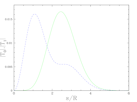
Figure 2: The absolute magnitude of the functions $T_{0}$ and $T_{1}$ for equilateral triangles as a function of the side length of the triangle, $s$. The solid green curve is $|T_{0}|$, and the dashed blue curve is $|T_{1}|$.

Fig. 2 shows the absolute value of $T_{0}$ and $T_{1}$ for equilateral triangles as a function of the triangle side length. Note that the $T_{i}$ are significant for triangles with side lengths up to about $4R$, so to measure $\mbox{$\langle M_{\rm ap}^{3}\rangle$}(R)$ up to $R=10\arcmin$, one would need a survey at least about $40\arcmin$ on a side. Interestingly, this is about the same size as one needs for the corresponding measurement of $\mbox{$\langle M_{\rm ap}^{2}\rangle$}(R)$.

Finally, we use the relations:

$$\langle M^{3}\rangle =\mbox{$\langle M_{\rm ap}^{3}\rangle$}+3i\mbox{$\langle M_{\rm ap}^{2}M_{\times}\rangle$}-3\mbox{$\langle M_{\rm ap}M_{\times}^{2}\rangle$}-i\mbox{$\langle M_{\times}^{3}\rangle$}$$ (53)

$$\langle M^{2}M^{*}\rangle =\mbox{$\langle M_{\rm ap}^{3}\rangle$}+i\mbox{$\langle M_{\rm ap}^{2}M_{\times}\rangle$}+\mbox{$\langle M_{\rm ap}M_{\times}^{2}\rangle$}+i\mbox{$\langle M_{\times}^{3}\rangle$}$$ (54)

to obtain:

$$\mbox{$\langle M_{\rm ap}^{3}\rangle$}(R) =\frac{1}{4}\Re\left(3\mbox{$\langle M^{2}M^{*}\rangle$}(R)+\mbox{$\langle M^{3}\rangle$}(R)\right)$$ (55)

$$\mbox{$\langle M_{\rm ap}^{2}M_{\times}\rangle$}(R) =\frac{1}{4}\Im\left(\mbox{$\langle M^{2}M^{*}\rangle$}(R)+\mbox{$\langle M^{3}\rangle$}(R)\right)$$ (56)

$$\mbox{$\langle M_{\rm ap}M_{\times}^{2}\rangle$}(R) =\frac{1}{4}\Re\left(\mbox{$\langle M^{2}M^{*}\rangle$}(R)-\mbox{$\langle M^{3}\rangle$}(R)\right)$$ (57)

$$\mbox{$\langle M_{\times}^{3}\rangle$}(R) =\frac{1}{4}\Im\left(3\mbox{$\langle M^{2}M^{*}\rangle$}(R)-\mbox{$\langle M^{3}\rangle$}(R)\right)$$ (58)

There is one further complication for using these formulae. In practice, one does not calculate $\Gamma_{i}(s,\mn@boldsymbol{t})$ for every $(s,\mn@boldsymbol{t})$, since this would include every triangle six times. A typical program would bin each triangle according to its shortest side, s, and its second shortest side, t, thus counting every triangle only once.

In this case, let us assume that we know $\Gamma_{i}(s,\mn@boldsymbol{t})$ for all $s$, but for only those $\mn@boldsymbol{t}$ where $|\mn@boldsymbol{t}~{}-~{}s|~{}>~{}t~{}>~{}s$. Then naively, Equation (45) becomes

$$\mbox{$\langle M^{3}\rangle$}(R)= \left[\int\frac{sds}{R^{2}}\int\limits_{s<t^{\prime}<|\mn@boldsymbol{t}^{\prime}-s|}\frac{d^{2}\mn@boldsymbol{t}^{\prime}}{2\pi R^{2}}\Gamma_{0}(s,\mn@boldsymbol{t}^{\prime})T_{0}\left(\frac{s}{R},\frac{\mn@boldsymbol{t}^{\prime}}{R}\right)\right.$$

$$+\int\frac{sds}{R^{2}}\int\limits_{s<|\mn@boldsymbol{t}^{\prime}-s|<t^{\prime}}\frac{d^{2}\mn@boldsymbol{t}^{\prime}}{2\pi R^{2}}\Gamma_{0}(s,s-\mn@boldsymbol{t}^{\prime})T_{0}\left(\frac{s}{R},\frac{s-\mn@boldsymbol{t}^{\prime}}{R}\right)$$

$$+\int\frac{sds}{R^{2}}\int\limits_{t^{\prime}<s<|\mn@boldsymbol{t}^{\prime}-s|}\frac{d^{2}\mn@boldsymbol{t}^{\prime}}{2\pi R^{2}}\Gamma_{0}\left(t^{\prime},\frac{s\mn@boldsymbol{t}^{\prime*}}{t^{\prime}}\right)T_{0}\left(\frac{t^{\prime}}{R},\frac{s\mn@boldsymbol{t}^{\prime*}}{t^{\prime}R}\right)$$

$$+\int\frac{sds}{R^{2}}\int\limits_{t^{\prime}<|\mn@boldsymbol{t}^{\prime}-s|<s}\frac{d^{2}\mn@boldsymbol{t}^{\prime}}{2\pi R^{2}}\Gamma_{0}\left(t^{\prime},\frac{(\mn@boldsymbol{t}^{\prime}-s)\mn@boldsymbol{t}^{\prime*}}{t^{\prime}}\right)T_{0}\left(\frac{t^{\prime}}{R},\frac{(\mn@boldsymbol{t}^{\prime}-s)\mn@boldsymbol{t}^{\prime*}}{t^{\prime}R}\right)$$

$$+\int\frac{sds}{R^{2}}\int\limits_{|\mn@boldsymbol{t}^{\prime}-s|<s<t^{\prime}}\frac{d^{2}\mn@boldsymbol{t}^{\prime}}{2\pi R^{2}}\Gamma_{0}\left(|\mn@boldsymbol{t}^{\prime}-s|,\frac{-s(\mn@boldsymbol{t}^{\prime}-s)^{*}}{|\mn@boldsymbol{t}^{\prime}-s|}\right)T_{0}\left(\frac{|\mn@boldsymbol{t}^{\prime}-s|}{R},\frac{-s(\mn@boldsymbol{t}^{\prime}-s)^{*}}{|\mn@boldsymbol{t}^{\prime}-s|R}\right)$$

$$\left.+\int\frac{sds}{R^{2}}\int\limits_{|\mn@boldsymbol{t}^{\prime}-s|<t^{\prime}<s}\frac{d^{2}\mn@boldsymbol{t}^{\prime}}{2\pi R^{2}}\Gamma_{0}\left(|\mn@boldsymbol{t}^{\prime}-s|,\frac{\mn@boldsymbol{t}^{\prime}(\mn@boldsymbol{t}^{\prime}-s)^{*}}{|\mn@boldsymbol{t}^{\prime}-s|}\right)T_{0}\left(\frac{|\mn@boldsymbol{t}^{\prime}-s|}{R},\frac{\mn@boldsymbol{t}^{\prime}(\mn@boldsymbol{t}^{\prime}-s)^{*}}{|\mn@boldsymbol{t}^{\prime}-s|R}\right)\right]$$ (59)

However, for each of these integrals, a change of variables transforms it into the first one. Thus, we have the much simpler result:

$$\mbox{$\langle M^{3}\rangle$}(R)=6\int\frac{sds}{R^{2}}\int\limits_{s<t^{\prime}<|\mn@boldsymbol{t}^{\prime}-s|}\frac{d^{2}\mn@boldsymbol{t}^{\prime}}{2\pi R^{2}}\Gamma_{0}(s,\mn@boldsymbol{t}^{\prime})T_{0}\left(\frac{s}{R},\frac{\mn@boldsymbol{t}^{\prime}}{R}\right)$$ (60)

The case is almost the same for $\langle M^{2}M^{*}\rangle$, except that the conjugated vertex changes in 4 of the integrals, so the net result is:

$$\mbox{$\langle M^{2}M^{*}\rangle$}(R) =2\int\frac{sds}{R^{2}}\int\limits_{s<t^{\prime}<|\mn@boldsymbol{t}^{\prime}-s|}\frac{d^{2}\mn@boldsymbol{t}^{\prime}}{2\pi R^{2}}\left[\Gamma_{1}(s,\mn@boldsymbol{t}^{\prime})T_{1}\left(\frac{s}{R},\frac{\mn@boldsymbol{t}^{\prime}}{R}\right)+\Gamma_{2}(s,\mn@boldsymbol{t}^{\prime})T_{2}\left(\frac{s}{R},\frac{\mn@boldsymbol{t}^{\prime}}{R}\right)+\Gamma_{3}(s,\mn@boldsymbol{t}^{\prime})T_{3}\left(\frac{s}{R},\frac{\mn@boldsymbol{t}^{\prime}}{R}\right)\right]$$ (61)

where $T_{2}$ and $T_{3}$ are obtained from $T_{1}$ by a cyclic rotation of the indices.

The extension to the kurtosis of the aperture mass ($\langle M_{\rm ap}^{4}\rangle(R)$) is straightforward and is given in the appendix.

4 Efficient Calculation of the Three-Point Correlation Function

4.1 Two-Point Algorithm

We consider an efficient algorithm for calculating the two-point correlation function first. This problem has been solved in a number of ways for the purposes of number count correlations for studying large-scale structure. Bertschinger (1998) gives a review of some techniques for that purpose. The algorithm we present below is most similar to that of Moore et al. (2000). There are a few complications due to the fact that we are correlating a vector field rather than a scalar number count, but the creation and use of the cells are quite analagous. Also, Zhang & Pen (2004) have recently presented a similar algorithm for the purposes of weak lensing. Therefore, we present a brief description of the algorithm below in order to describe the unique features of our version of the algorithms, and we defer to these other two papers for more comprehensive descriptions of the general method.

The most naive algorithm for calculating the two-point correlation function would be to take every pair of galaxies in the field and put the product of the shears into a bin corresponding to their separation. Then the average value could be found for each bin. Clearly, this is extremely slow for large datasets, being an $O(N^{2})$ algorithm. The corresponding three-point algorithm is even worse, $O(N^{3})$.

However, we note that the binning inherent in even this brute-force technique is effectively smoothing the correlation function by the size of the bins, since we lose all information about where within each bin the pair really belongs. If we allow ourselves to smooth again on this scale, then we can greatly speed up the algorithm.

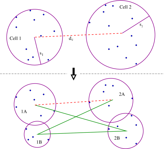
First, binning is usually done in logarithmic bins in the separation, $d$, with some specified minimum and maximum scale, $d_{min}<d<d_{max}$. Now, suppose we have two circular regions of radii $s_{1}$ and $s_{2}$, whose centres are separated by a distance $d_{c}$. Then, then the separation for any pair of galaxies taken from these two regions must fall in the range $d_{c}-s_{1}-s_{2}<d<d_{c}+s_{1}+s_{2}$. If the radii are much less than $d$, this becomes

$$\ln(d_{c})-\frac{s_{1}+s_{2}}{d_{c}}<\ln(d)<\ln(d_{c})+\frac{s_{1}+s_{2}}{d_{c}}$$ (62)

So, if our regions satisfy

$$\frac{s_{1}+s_{2}}{d_{c}}<b$$ (63)

where $b\equiv\Delta({\rm ln}d)$ is the bin size, then we can put all of them into the same bin, knowing that we will be wrong by at most one bin for any specific pair of galaxies.

In this case, we can take the average of the shear values in each region and place the product of the averages in our bin, dropping the calculation time for these galaxies from $O(N_{1}N_{2})$ to $O(N_{1}+N_{2})$, where $N_{1}$ and $N_{2}$ are the number of galaxies in each region. When the $N$’s are large, this can be a huge speedup.

The specific technique for implementing this type of algorithm is to create a so-called kd-tree (with k=2 in this case) for the data. Again, we defer to Moore et al. (2000) and Zhang & Pen (2004) for a more complete description of this type of data structure.

In short, we bin the data in ‘Cells’, keeping track of various average values for the galaxies in each Cell along with its centroid and size (maximum distance of a galaxy from the centroid). Each Cell with more than one galaxy (and larger than $d_{\rm min}$) also contains pointers to two sub-Cells with half the number of galaxies each.

When Equation (63) is not satisfied, we split each Cell (roughly) in half and check the resulting pairs of regions. Cell splitting continues in this manner until all pairs can be calculated directly. Note that the recursion must stop at some point, since $s_{1}+s_{2}=0$ for two individual galaxies, so Equation (63) must be satisfied eventually.

Figure 3: A sample calculation step in the two-point algorithm. At first the two Cells are too large compared to the distance between them, so they need to be split up. After the splits, there are four pairs of subcells to be considered. Three of the pairs (marked with green solid lines) satisfy Equation (63), and thus can be computed directly. The fourth (marked with a red dashed line) needs to be split again.

Fig. 3 shows an example of a splitting decision in the algorithm. At this point we are calculating the correlation between all the points in Cell 1 with all the points in Cell 2. In the top half of the figure, $s_{1}+s_{2}$ is too large compared to $d_{c}$, so we split both Cells into their subcells. There are now 4 pairs of subcells to consider. The three marked by the green solid line now satisfy Equation (63), and can be calculated directly. But the 1A-2A pair marked by the red dashed line needs to be split again.

We tested this algorithm on a 2.4 GHz Xeon processor for a square field 200 arcminutes on a side, and found the calculation time and memory usage to be:

$$T \approx 3.6\left(\frac{N}{10^{5}}\right)^{1.0}\left(\frac{b}{0.1}\right)^{-1.7}\text{seconds}$$ (64)

$$M \approx 19\left(\frac{N}{10^{5}}\right)^{1.0}\text{MB}$$ (65)

Even for $N\approx 10^{8}$, which will be required for surveys like those of the Supernova Anisotropy Probe (SNAP) and the Large-aperture Synoptic Survey Telescope (LSST), this algorithm still only takes about an hour and uses less than 20 GB of memory, which we expect will be common on destop computers by the time such surveys become available. Therefore, we do not foresee any need to improve upon this algorithm in the near future.

4.2 Three-Point Algorithm

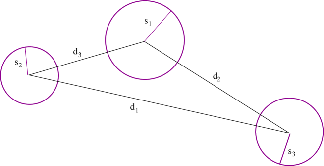
For the three-point function, the triangles are parametrized by three values (since we ignore any overall rotation or translation). One possible parametrization would be to use the three side lengths: $d_{1}>d_{2}>d_{3}$. This is not a good choice for two reasons. First, the orientation of the points is lost - a non-isocolese triangle is not distinguished from its mirror image. Second, the range of the parameters is a function of the other parameter values (e.g. $d_{1}-d_{2}<d_{3}<d_{2}$).

A better choice is the following for a triangle with $d_{1}>d_{2}>d_{3}$:

$$r =d_{3} \qquad r_{\rm min}<r <r_{\rm max}$$ (66)

$$u =d_{3}/d_{2} 0<u <1$$ (67)

$$v =\pm(d_{1}-d_{2})/d_{3} -1<v <1$$ (68)

where v is positive when $(\mn@boldsymbol{x}_{1},\mn@boldsymbol{x}_{2},\mn@boldsymbol{x}_{3})$ are oriented counter-clockwise and negative when clockwise.

Figure 4: The geometry of the triangle in the discussion of the three-point algorithm. We use the slightly non-intuitive convention that $d_{1}>d_{2}>d_{3}$ (rather than the other way around). This is so we agree with Fig. 1 with s as the smallest side, as desired for Equations 60 and 61.

We bin uniformly in ln($r$), $u$ and $v$ with a bin size $b$. Now, if we have three circular regions of radii $s_{1},s_{2},s_{3}$, whose centres make a triangle with $d_{1}>d_{2}>d_{3}$ (see Fig. 4), we can use the average shear in each when all of the following conditions hold:

$$\frac{s_{1}+s_{2}}{d_{3}} <b$$ (69)

$$\frac{s_{3}}{d_{2}} <\frac{b}{u}$$ (70)

$$\frac{s_{3}}{d_{2}} <\frac{b}{\sqrt{1-v^{2}}}$$ (71)

When considering three Cells for calculating the correlation function, if the sizes satisfy the above criteria, we use the average shears for each and place the product into the bin corresponding to the triangle formed by their centres. Otherwise, we recurse down to the sub-Cells of (some or all of) the Cells and try again.

This algorithm is far faster than the naive brute-force approach of taking every triple of galaxies which would be $O(N^{3})$. For the same field and processor mentioned above, we find the computation time and memory usage for our implementation of this algorithm to be:

$$T \approx 415\left(\frac{N}{10^{5}}\right)^{1.4}\left(\frac{b}{0.1}\right)^{-3.3}\text{minutes}$$ (72)

$$M \approx 22\left(\frac{N}{10^{5}}\right)^{1.0}\text{MB}$$ (73)

Zhang & Pen (2004) show some empirical computation times for their algorithm as well, which are shown in their fig. 3. Although their tests were made at somewhat lower values of $N$ than our tests, we believe that their scaling law at the same fiducial values we quote above is likely to be similar to ours.

The algorithm takes the most time dealing with triangles which are a significant fraction of the size of the field. So for very large fields, when one is only interested in the correlation on small scales, the calculation will be somewhat faster than this, as the larger triangles can be ignored.

4.3 A Faster Algorithm

We have discovered a way to significantly improve upon this algorithm, at least for large values of $N$. However, it can require a significant amount of memory, so depending on one’s computing resources and survey size, it may not always be a viable option.

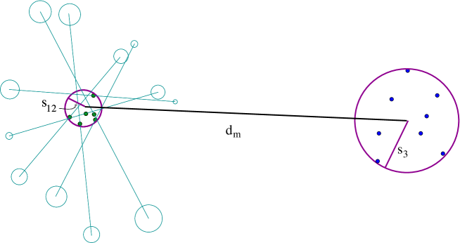
Figure 5: The geometry of the PairCell’s for the improved three-point algorithm. The pairs on the left side of the figure all have midpoints which are near each other, and have cells at roughly the same separation. Thus, they all fall into a single PairCell. The dots represent the midpoints of each pair. The size of the PairCell, $s_{12}$, is based on the scatter of these midpoints. The distance from the PairCell to another Cell is then the median of the corresponding triangles, $d_{m}$.

In this algorithm, we proceed one bin at a time in $\ln(r)$ rather than doing all at once as we did in the above algorithm. For each bin, we find all pairs of Cells with $(s_{1}+s_{2})/d_{3}<b$ where $d_{3}$ falls in the bin in question. Then, we find the midpoint $M$ of each pair, and create a new kd-tree for these pairs using these $M$’s for the positions of each pair. (See Fig. 5.)

Then, each ‘PairCell’ refers to a collection of pairs. For each, we keep track of the mean $M$ position, and the scatter of the $M$’s, which we call $s_{12}$. We don’t average the data for all of the pairs in the bin, since the triangles made from these pairs and a third point can still have very different shapes depending on the orientation of the pair. But two pair with similar orientations will go into the same $r,u,v$ bin. Therefore, within each PairCell, we bin the pairs according to their orientation, using a total of 4/b bins in order to maintain our rule of being off by at most one bin in u and v.

Finally we correlate the PairCell data with the third points of the triangles by traversing the tree of pairs and the original tree of Cells described above. For a given PairCell with size $s_{12}$ and a normal Cell with size $s_{3}$, separated by a distance $d_{m}$, we split one or both unless

$$\frac{s_{12}+s_{3}}{d_{m}}<b$$ (74)

Note that for each PairCell and Cell which satisfy this requirement, the various pair orientations stored in the PairCell span the entire range of $-1<v<1$. Also, if $d_{3}/d_{m}$ is not very small, we need to calculate $u$ separately for each orientation as well, since $u$ can vary by several bin sizes. But for each individual orientation, the above equation guarantees that we are only smoothing by one bin in $u$ or $v$.

When one typically has many pairs in each PairCell at the point where Equation (74) holds, then this algorithm would be expected to be significantly faster than our previous algorithm, which effectively does each pair individually. This is usually true for the large triangles where the algorithm spends the most time, so we find that this algorithm does turn out to be significantly faster than our previous one.

Empirically, the calculation time and memory usage for this algorithm are found to be:

$$T \approx 161\left(\frac{N}{10^{5}}\right)^{1.1}\left(\frac{b}{0.1}\right)^{-3.7}\text{minutes}$$ (75)

$$M \approx 800\left(\frac{N}{10^{5}}\right)^{1.0}\left(\frac{b}{0.1}\right)^{-1.2}\text{MB}$$ (76)

This is a factor of 2.6 faster than the previous algorithm for our fiducial values, and the speedup increases with $N$, since it scales as a smaller power of $N$ than our previous algorithm.

However, for fields with $N>10^{6}$, the memory demands become difficult for a desktop machine (although still feasible with modern supercomputers). For the SNAP or LSST surveys with $N\approx 10^{8}$, this algorithm will require almost a terabyte of memory. This would be a lot by today’s standards, but when the data from these surveys eventually become available, it will probably be quite manageable. Likewise, this algorithm would take a good fraction of a year for the desktop machine described above, but in five or ten years, it will must faster. In any case, this algorithm is extrapolated to be about 20 times faster than the previous algorithm.

If anyone is interested in the code for any of these algorithms or would like to use our code on a survey dataset, we would be happy to provide it for you. If interested, please send an email to Mike Jarvis (mjarvis@hep.upenn.edu).

5 Application to Simulated and Observed Data

5.1 Simulated Shear

To verify that the above equations are correct, we first apply them to a simulated shear field produced by ray tracing simulations (Jain, Seljak & White, 2000). The simulated data uniformly cover an area $200\arcmin$ on a side, and have no shape noise on the shear values. The particular simulation we used was for $\Lambda$CDM with $\Omega_{m}=0.3$, $\Lambda=0.7$, $\Gamma=0.21$ and $\sigma_{8}=0.9$, with sources at $z=1$.

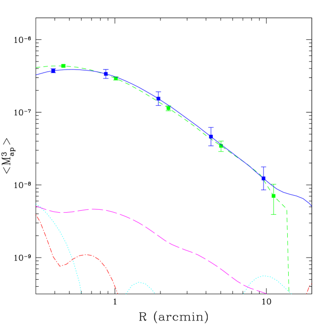
We measure $\langle M_{\rm ap}^{3}\rangle$ both from the correlation functions as described above and also by measuring $M_{\rm ap}$ for many apertures using Equation (2) and then computing $\langle M_{\rm ap}^{3}\rangle$ directly. This second technique is not possible on real data, due to masking effects from bright stars or complicated survey geometry, as discussed in §1, but for the simulated data, there is no masking, so the direct computation is possible.

Figure 6: A comparison between a direct calculation of $\langle M_{\rm ap}^{3}\rangle$ and the integration technique presented in this paper for a simulated shear field with no shape noise or masking. The direct calculation is the green dashed curve, and the integration technique is the blue solid curve. The three other curves near (and often below) the bottom of the plot are the absolute values of the mixed and B-modes measured by the integration technique.

The results from the two methods are shown in Fig. 6. The results from the direct aperture method (Equation (2)) are the dashed green curve. The results from the integration method (§3) using $b=0.1$ are the solid blue curve. The error bars for the direct method were estimated from the distribution of $M_{\rm ap}$ values used to compute the average. For the integration technique, we took 12 samples of 100,000 points drawn from the gridded simulation field, and computed the error bars from the actual ‘field-to-field’ variance. The sampling is needed to prevent the gridding signature of the simulation from showing up in the correlation functions and affecting the results.

The two methods are seen to agree to within the error bars over most of the range, so we believe the formulae in §3 to be accurate. The largest discrepency is at scales just above $10\arcmin$ where the direct measurement abruptly falls off. We think that this is due to there being too few apertures in the field to accurately calculate the skewness. At $R=10\arcmin$, $U_{R}(r)$ is significant out to $20\arcmin$, so one can only fit 5 non-overlapping apertures of this size within the $200\arcmin$ square. We do use overlapping apertures for our calculation, since the measurements should still be nearly independent when the apertures overlap somewhat, but we believe that the relatively small number of independent apertures is likely to be the source of the discrepency.

The figure also shows the mixed and B-modes measured by the integration technique: $\langle M_{\rm ap}^{2}M_{\times}\rangle$ is the cyan dotted curve, $\langle M_{\rm ap}M_{\times}^{2}\rangle$ is the magenta long dashed curve, and $\langle M_{\times}^{3}\rangle$ is the red dot-dashed curve. The plotted values are the absolute values of the measurements, and the largest of these ($\langle M_{\rm ap}M_{\times}^{2}\rangle$) is roughly two orders of magnitude below the E-mode signal. This is due to the use of $b=0.1$; using a smaller value would reduce the leakage of power from the E-mode to the others still further.

5.2 CTIO Survey Data

We next apply the above formulae to our 75 square degree CTIO (Cerro Tololo Interamerican Observatory) survey. A complete description of the survey data and the processing techniques used is found in Jarvis et al. (2003). The 75 total square degrees are divided among 12 fields, each roughly 2.5 degrees square. Each field has of order 150,000 usable galaxies. We have also corrected the error pointed out by Hirata & Seljak (2003) in our dillution correction formula. The data presented here use their linear approximation for this correction, which they find to be significantly more accurate than our formula.

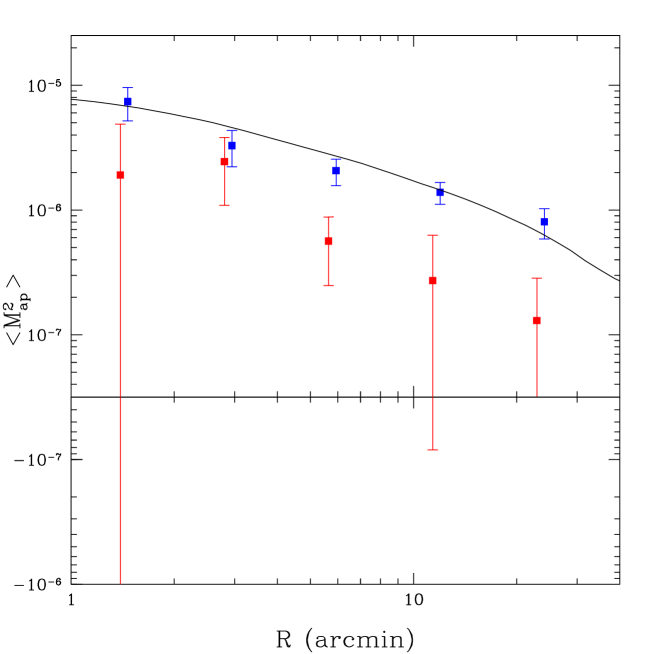
In our previous paper, we measured the $\langle M_{\rm ap}^{2}\rangle$ statistic and found a clear detection of the E-mode signal, but found significant B-mode as well. We had used the aperture mass definition of Schneider et al. (2002) rather than the one defined herein (Equation (1)), so we present the results for this definition in Fig. 7. The E-mode ($\langle M_{\rm ap}^{2}\rangle$) is shown in blue, and the B-mode ($\langle M_{\times}^{2}\rangle$) in red. The measurements shown are spaced by approximately a factor of 2 in $R$, since this is where the measurements become independent of each other.(Schneider et al., 2002). Note that the error bars are calculated from field-to-field variation, so they accurately represent both statistical and sample variance.

Figure 7: The variance of the aperture mass statistic using the integration technique for our CTIO 75 square degree survey. The E-mode component is blue, and the B-mode component is red. As discussed in Jarvis et al. (2003), there is evidently significant B-mode contamination at scales less than $10\arcmin$. The black curve is the theoretical prediction for the concordance $\Lambda$CDM model.

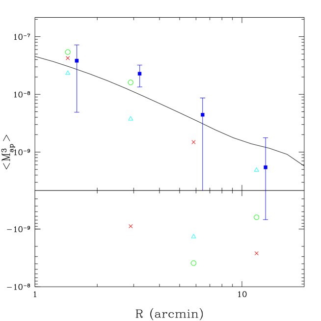
Our calculation of the $\langle M_{\rm ap}^{3}\rangle$ statistic, as well as the mixed and B-mode statistics, are shown in Fig. 8 for the range of $1\arcmin<R<20\arcmin$. Less than $1\arcmin$, the B-mode contamination in the two-point measurement became large compared to the signal. And greater than $20\arcmin$, we do not fully trust the measurement, since this is where the integration and direct measurements differed for the simulated field described above.

With the integration technique, we can calculate a value for $\langle M_{\rm ap}^{3}\rangle$ at any value of $R$. However, as with the variance, we plot them spaced by a factor of 2 in $R$, since this is when the points become uncorrelated. Also, the error bars are again calculated from the field-to-field variation, so they inlude sample variance. We omit the error bars for the mixed and B-modes for the sake of clarity, but their size is similar to those of the E-mode errors.

Figure 8: The skewness of the aperture mass statistic using the integration technique for our CTIO 75 square degree survey. The E-mode ($\langle M_{\rm ap}^{3}\rangle$) is shown in blue, with error bars indicating the field-to-field variance of the measurement. The mixed and B-modes are the circles ($\langle M_{\rm ap}^{2}M_{\times}\rangle$), triangles ($\langle M_{\rm ap}M_{\times}^{2}\rangle$), and crosses ($\langle M_{\times}^{2}\rangle$). The black curve is the theoretical prediction for the concordance $\Lambda$CDM model.

Unfortunately, the detection is fairly marginal. The best conclusion we can draw is that $\langle M_{\rm ap}^{3}\rangle$ is roughly the right order of magnitude to be consistent with a concordance $\Lambda$CDM model, given as the solid black curve in Fig. 8. (We scaled the measurements from the above simulation to $\sigma_{8}=0.8$ and to $z_{s}=0.6$ based on the theoretical scaling found by Takada & Jain (2002).) However, the S/N is quite low, and the mixed and B-modes indicate that there are potentially significant systematic errors contaminating the results. Thus, we do not try to use this result to constrain any cosmological models.

One test we are willing to make with this data is to test whether it is consistent with zero. The statistic we use for this test is:

$$P=\frac{1}{N}\sum{\frac{\mbox{$\langle M_{\rm ap}^{3}\rangle$}(R_{i})}{\sigma_{i}}}$$ (77)

Over the range plotted, we find that $P=1.09\pm 0.48$, which is a detection at the $2.3\sigma$ level. The other three modes give values of 0.31, 0.14 and -0.13, all within $1\sigma$ of zero. So, we do have a mildly significant detection that the skewness is positive, but we cannot make any stronger claim than that.

6 Conclusion

We have presented a new calculation for the skewness of the aperture mass as an integral over the more easily measured three-point correlation function. We have also presented efficient algorithms for calculating the three-point correlation function in real data. These algorithms are believed to be faster than other published algorithms. Finally, we have applied these methods to our CTIO survey data, for which we do not obtain a strong detection. The signal is consistent with the concordance model prediction, but is only inconsistent with zero at the $2\sigma$ level.

However, we expect that this method will be useful for ongoing and future surveys which are deeper and wider than ours, and will therefore be better able to detect the signal. Pen et al. (2003) have already used a similar technique on the VIRMOS/DESCART survey, and have measured an E-mode signal which is significantly greater than the mixed and B-mode contaminations (at least for some values of R). They find $\Omega_{m}<0.5$ at 90 per cent confidence.

There are several ongoing and proposed surveys which will substantially increase the S/N in these measurements. For example, the Canada-France Legacy Survey (CFLS) will cover 170 square degrees at a depth of $r<25.7$. This is a similar depth to the VIRMOS/DESCART survey, but covers about 20 times more area, so the S/N would be expected to increase by a factor of 4.

The CFLS will observe three disjoint fields, two of 49 square degrees and one of 72 square degrees, with an estimated number of galaxies of roughly 600,000 and 900,000 respectively. Thus, the total calculation time for our fastest three-point algorithm will be about 3 days and require a maximum of about 7 GB of memory on a modern desktop computer, which is quite feasible.

In fact, this would calculate the correlation function for the entire range of scales available (up to 7 or 8 degrees), which is not necessary. Limiting the calculation to scales less than about 200 arcmin, where the signal is strongest, speeds up the calculation significantly. In the current implementation, this would not reduce the algorithm’s memory demand, but one could easily modify the algorithm to keep only a fraction of the total galaxies in memory at a time which would be useful for surveys such as this one with large contiguous fields.

Improvements in the reduction techniques are probably just as important as increasing the number of galaxies, since the B-mode contamination is evidence that there are still some systematic errors in the data. So far all surveys who have checked for B-modes in the data show this contamination at a significant level, although there are often scales at which the B-mode is small compared to the E-mode signal. Reducing these systematic effects will probably require both better PSF-removal algorithms as well as cleaner raw images.

Appendix A Kurtosis

The calculation of the fourth moment of the aperture mass can likewise be made from the four-point correlation function:

$$\mbox{$\langle M^{4}\rangle$}(R) =24\int\frac{sds}{R^{2}}\int\limits_{s<t^{\prime}<|\mn@boldsymbol{t}^{\prime}-s|}\frac{d^{2}\mn@boldsymbol{t}^{\prime}}{2\pi R^{2}}\int\limits_{t^{\prime}<u^{\prime},t^{\prime}<|\mn@boldsymbol{u}^{\prime}-s|}\frac{d^{2}\mn@boldsymbol{u}^{\prime}}{2\pi R^{2}}\Gamma^{(4)}_{0}(s,\mn@boldsymbol{t}^{\prime},\mn@boldsymbol{u}^{\prime})T^{(4)}_{0}\left(\frac{s}{R},\frac{\mn@boldsymbol{t}^{\prime}}{R},\frac{\mn@boldsymbol{u}^{\prime}}{R}\right)$$ (78)

$$\mbox{$\langle M^{3}M^{*}\rangle$}(R) =6\int\frac{sds}{R^{2}}\int\limits_{s<t^{\prime}<|\mn@boldsymbol{t}^{\prime}-s|}\frac{d^{2}\mn@boldsymbol{t}^{\prime}}{2\pi R^{2}}\int\limits_{t^{\prime}<u^{\prime},t^{\prime}<|\mn@boldsymbol{u}^{\prime}-s|}\frac{d^{2}\mn@boldsymbol{u}^{\prime}}{2\pi R^{2}}\left[\Gamma^{(4)}_{1}(s,\mn@boldsymbol{t}^{\prime},\mn@boldsymbol{u}^{\prime})T^{(4)}_{1}\left(\frac{s}{R},\frac{\mn@boldsymbol{t}^{\prime}}{R},\frac{\mn@boldsymbol{u}^{\prime}}{R}\right)\right.$$

$$\qquad\left.+\Gamma^{(4)}_{2}(s,\mn@boldsymbol{t}^{\prime},\mn@boldsymbol{u}^{\prime})T^{(4)}_{2}\left(\frac{s}{R},\frac{\mn@boldsymbol{t}^{\prime}}{R},\frac{\mn@boldsymbol{u}^{\prime}}{R}\right)+\Gamma^{(4)}_{3}(s,\mn@boldsymbol{t}^{\prime},\mn@boldsymbol{u}^{\prime})T^{(4)}_{3}\left(\frac{s}{R},\frac{\mn@boldsymbol{t}^{\prime}}{R},\frac{\mn@boldsymbol{u}^{\prime}}{R}\right)+\Gamma^{(4)}_{4}(s,\mn@boldsymbol{t}^{\prime},\mn@boldsymbol{u}^{\prime})T^{(4)}_{4}\left(\frac{s}{R},\frac{\mn@boldsymbol{t}^{\prime}}{R},\frac{\mn@boldsymbol{u}^{\prime}}{R}\right)\right]$$ (79)

$$\mbox{$\langle M^{2}M^{*2}\rangle$}(R) =8\int\frac{sds}{R^{2}}\int\limits_{s<t^{\prime}<|\mn@boldsymbol{t}^{\prime}-s|}\frac{d^{2}\mn@boldsymbol{t}^{\prime}}{2\pi R^{2}}\int\limits_{t^{\prime}<u^{\prime},t^{\prime}<|\mn@boldsymbol{u}^{\prime}-s|}\frac{d^{2}\mn@boldsymbol{u}^{\prime}}{2\pi R^{2}}\left[\Gamma^{(4)}_{5}(s,\mn@boldsymbol{t}^{\prime},\mn@boldsymbol{u}^{\prime})T^{(4)}_{5}\left(\frac{s}{R},\frac{\mn@boldsymbol{t}^{\prime}}{R},\frac{\mn@boldsymbol{u}^{\prime}}{R}\right)\right.$$

$$\qquad\left.+\Gamma^{(4)}_{6}(s,\mn@boldsymbol{t}^{\prime},\mn@boldsymbol{u}^{\prime})T^{(4)}_{6}\left(\frac{s}{R},\frac{\mn@boldsymbol{t}^{\prime}}{R},\frac{\mn@boldsymbol{u}^{\prime}}{R}\right)+\Gamma^{(4)}_{7}(s,\mn@boldsymbol{t}^{\prime},\mn@boldsymbol{u}^{\prime})T^{(4)}_{7}\left(\frac{s}{R},\frac{\mn@boldsymbol{t}^{\prime}}{R},\frac{\mn@boldsymbol{u}^{\prime}}{R}\right)\right]$$ (80)

where we define the natural components of the four-point correlation function as did Schneider & Lombardi (2002) (although our ordering is different):

$$\Gamma^{(4)}_{0}(s,\mn@boldsymbol{t}^{\prime},\mn@boldsymbol{u}^{\prime}) =\langle\gamma(\mn@boldsymbol{r})\gamma(\mn@boldsymbol{r}+\mn@boldsymbol{s})\gamma(\mn@boldsymbol{r}+\mn@boldsymbol{t})\gamma(\mn@boldsymbol{r}+\mn@boldsymbol{u})e^{-8i\alpha}\rangle$$ (81)

$$\Gamma^{(4)}_{1}(s,\mn@boldsymbol{t}^{\prime},\mn@boldsymbol{u}^{\prime}) =\langle\gamma(\mn@boldsymbol{r})^{*}\gamma(\mn@boldsymbol{r}+\mn@boldsymbol{s})\gamma(\mn@boldsymbol{r}+\mn@boldsymbol{t})\gamma(\mn@boldsymbol{r}+\mn@boldsymbol{u})e^{-4i\alpha}\rangle$$ (82)

$$\Gamma^{(4)}_{2}(s,\mn@boldsymbol{t}^{\prime},\mn@boldsymbol{u}^{\prime}) =\langle\gamma(\mn@boldsymbol{r})\gamma(\mn@boldsymbol{r}+\mn@boldsymbol{s})^{*}\gamma(\mn@boldsymbol{r}+\mn@boldsymbol{t})\gamma(\mn@boldsymbol{r}+\mn@boldsymbol{u})e^{-4i\alpha}\rangle$$ (83)

$$\Gamma^{(4)}_{3}(s,\mn@boldsymbol{t}^{\prime},\mn@boldsymbol{u}^{\prime}) =\langle\gamma(\mn@boldsymbol{r})\gamma(\mn@boldsymbol{r}+\mn@boldsymbol{s})\gamma(\mn@boldsymbol{r}+\mn@boldsymbol{t})^{*}\gamma(\mn@boldsymbol{r}+\mn@boldsymbol{u})e^{-4i\alpha}\rangle$$ (84)

$$\Gamma^{(4)}_{4}(s,\mn@boldsymbol{t}^{\prime},\mn@boldsymbol{u}^{\prime}) =\langle\gamma(\mn@boldsymbol{r})\gamma(\mn@boldsymbol{r}+\mn@boldsymbol{s})\gamma(\mn@boldsymbol{r}+\mn@boldsymbol{t})\gamma(\mn@boldsymbol{r}+\mn@boldsymbol{u})^{*}e^{-4i\alpha}\rangle$$ (85)

$$\Gamma^{(4)}_{5}(s,\mn@boldsymbol{t}^{\prime},\mn@boldsymbol{u}^{\prime}) =\langle\gamma(\mn@boldsymbol{r})^{*}\gamma(\mn@boldsymbol{r}+\mn@boldsymbol{s})^{*}\gamma(\mn@boldsymbol{r}+\mn@boldsymbol{t})\gamma(\mn@boldsymbol{r}+\mn@boldsymbol{u})\rangle$$ (86)

$$\Gamma^{(4)}_{6}(s,\mn@boldsymbol{t}^{\prime},\mn@boldsymbol{u}^{\prime}) =\langle\gamma(\mn@boldsymbol{r})^{*}\gamma(\mn@boldsymbol{r}+\mn@boldsymbol{s})\gamma(\mn@boldsymbol{r}+\mn@boldsymbol{t})^{*}\gamma(\mn@boldsymbol{r}+\mn@boldsymbol{u})\rangle$$ (87)

$$\Gamma^{(4)}_{7}(s,\mn@boldsymbol{t}^{\prime},\mn@boldsymbol{u}^{\prime}) =\langle\gamma(\mn@boldsymbol{r})^{*}\gamma(\mn@boldsymbol{r}+\mn@boldsymbol{s})\gamma(\mn@boldsymbol{r}+\mn@boldsymbol{t})\gamma(\mn@boldsymbol{r}+\mn@boldsymbol{u})^{*}\rangle$$ (88)

The corresponding $T$ functions are:

$$T^{(4)}_{0}(s,\mn@boldsymbol{t}^{\prime},\mn@boldsymbol{u}^{\prime}) =\frac{\mn@boldsymbol{q}_{1}^{*2}\mn@boldsymbol{q}_{2}^{*2}\mn@boldsymbol{q}_{3}^{*2}\mn@boldsymbol{q}_{4}^{*2}}{64}\exp\left(-\frac{q_{1}^{2}+q_{2}^{2}+q_{3}^{2}+q_{4}^{2}}{2}\right)$$ (89)

$$T^{(4)}_{1}(s,\mn@boldsymbol{t}^{\prime},\mn@boldsymbol{u}^{\prime}) =\left[\frac{\mn@boldsymbol{q}_{2}^{*2}\mn@boldsymbol{q}_{3}^{*2}+\mn@boldsymbol{q}_{2}^{*2}\mn@boldsymbol{q}_{4}^{*2}+\mn@boldsymbol{q}_{3}^{*2}\mn@boldsymbol{q}_{4}^{*2}-4\mn@boldsymbol{q}_{1}^{*}\mn@boldsymbol{q}_{2}^{*}\mn@boldsymbol{q}_{3}^{*}\mn@boldsymbol{q}_{4}^{*}}{128}+\frac{\mn@boldsymbol{q}_{1}\mn@boldsymbol{q}_{2}^{*}\mn@boldsymbol{q}_{3}^{*}\mn@boldsymbol{q}_{4}^{*}(\mn@boldsymbol{q}_{2}^{*}\mn@boldsymbol{q}_{3}^{*}+\mn@boldsymbol{q}_{2}^{*}\mn@boldsymbol{q}_{4}^{*}+\mn@boldsymbol{q}_{3}^{*}\mn@boldsymbol{q}_{4}^{*})}{32}\right.$$

$$\qquad\left.+\frac{\mn@boldsymbol{q}_{1}^{2}\mn@boldsymbol{q}_{2}^{*2}\mn@boldsymbol{q}_{3}^{*2}\mn@boldsymbol{q}_{4}^{*2}}{64}\right]\exp\left(-\frac{q_{1}^{2}+q_{2}^{2}+q_{3}^{2}+q_{4}^{2}}{2}\right)$$ (90)

$$T^{(4)}_{2-4}(s,\mn@boldsymbol{t}^{\prime},\mn@boldsymbol{u}^{\prime}) =T^{(4)}_{1}(s,\mn@boldsymbol{t}^{\prime},\mn@boldsymbol{u}^{\prime})~{}\text{after a cyclic rotation of indices (1,2,3,4)}$$ (91)

$$T^{(4)}_{5}(s,\mn@boldsymbol{t}^{\prime},\mn@boldsymbol{u}^{\prime}) =\left[\frac{(2\mn@boldsymbol{q}_{1}^{*}\mn@boldsymbol{q}_{2}^{*}+(\mn@boldsymbol{q}_{1}^{*}+\mn@boldsymbol{q}_{2}^{*})^{2})(2\mn@boldsymbol{q}_{3}^{*}\mn@boldsymbol{q}_{4}^{*}+(\mn@boldsymbol{q}_{3}^{*}+\mn@boldsymbol{q}_{4}^{*})^{2})-6|\mn@boldsymbol{q}_{3}+\mn@boldsymbol{q}_{4}|^{2}+3}{128}\right.$$

$$\qquad\left.-\frac{\mn@boldsymbol{q}_{1}\mn@boldsymbol{q}_{2}\mn@boldsymbol{q}_{3}^{*}\mn@boldsymbol{q}_{4}^{*}|\mn@boldsymbol{q}_{3}+\mn@boldsymbol{q}_{4}|^{2})}{32}+\frac{\mn@boldsymbol{q}_{1}^{2}\mn@boldsymbol{q}_{2}^{2}\mn@boldsymbol{q}_{3}^{*2}\mn@boldsymbol{q}_{4}^{*2}}{64}\right]\exp\left(-\frac{q_{1}^{2}+q_{2}^{2}+q_{3}^{2}+q_{4}^{2}}{2}\right)$$ (92)

$$T^{(4)}_{6-7}(s,\mn@boldsymbol{t}^{\prime},\mn@boldsymbol{u}^{\prime}) =T^{(4)}_{5}(s,\mn@boldsymbol{t}^{\prime},\mn@boldsymbol{u}^{\prime})~{}\text{after a cyclic rotation of indices (2,3,4)}$$ (93)

where the $q$’s are again the vectors from each vertex to the centroid:

$$\mn@boldsymbol{q}_{1} =(s+\mn@boldsymbol{t}^{\prime}+\mn@boldsymbol{u}^{\prime})/4$$ (94)

$$\mn@boldsymbol{q}_{2} =(\mn@boldsymbol{t}^{\prime}+\mn@boldsymbol{u}^{\prime}-3s)/4$$ (95)

$$\mn@boldsymbol{q}_{3} =(s+\mn@boldsymbol{u}^{\prime}-3\mn@boldsymbol{t}^{\prime})/4$$ (96)

$$\mn@boldsymbol{q}_{4} =(s+\mn@boldsymbol{t}^{\prime}-3\mn@boldsymbol{u}^{\prime})/4$$ (97)

Finally, we can obtain the moments of $M_{\rm ap}$ and $M_{\times}$ from:

$$\mbox{$\langle M_{\rm ap}^{4}\rangle$}(R) =\frac{1}{8}\Re\left(\mbox{$\langle M^{4}\rangle$}(R)+4\mbox{$\langle M^{3}M^{*}\rangle$}(R)+3\mbox{$\langle M^{2}M^{*2}\rangle$}(R)\right)$$ (98)

$$\mbox{$\langle M_{\rm ap}^{3}M_{\times}\rangle$}(R) =\frac{1}{8}\Im\left(\mbox{$\langle M^{4}\rangle$}(R)+2\mbox{$\langle M^{3}M^{*}\rangle$}(R)\right)$$ (99)

$$\mbox{$\langle M_{\rm ap}^{2}M_{\times}^{2}\rangle$}(R) =\frac{1}{8}\Re\left(-\mbox{$\langle M^{4}\rangle$}(R)+\mbox{$\langle M^{2}M^{*2}\rangle$}(R)\right)$$ (100)

$$\mbox{$\langle M_{\rm ap}M_{\times}^{3}\rangle$}(R) =\frac{1}{8}\Im\left(-\mbox{$\langle M^{4}\rangle$}(R)+2\mbox{$\langle M^{3}M^{*}\rangle$}(R)\right)$$ (101)

$$\mbox{$\langle M_{\times}^{4}\rangle$}(R) =\frac{1}{8}\Re\left(\mbox{$\langle M^{4}\rangle$}(R)-4\mbox{$\langle M^{3}M^{*}\rangle$}(R)+3\mbox{$\langle M^{2}M^{*2}\rangle$}(R)\right)$$ (102)

References

• Bernardeau et al. (1997) Bernardeau F., van Waerbeke L., Mellier Y., 1997, A&A, 332, 1
• Bernardeau et al. (2002) Bernardeau F., Mellier, Y., van Waerbeke L., 2002, A&A, 389, 28
• Bertschinger (1998) Bertschinger E., 1998, ARA&A, 36, 599
• Crittenden et al. (2002) Crittenden R., Natarajan P, Pen U., Theuns T., 2002, ApJ, 568, 20
• Hamana et al. (2003) Hamana T., Miyazaki S., Shimasaku K., Furusawa H., Doi M., Hamabe M., Imi K., Kimura M., Komiyama Y., Nakata F., Okada N., Okamura S., Ouchi M., Sekiguchi M., Yagi M., Yasuda N., 2003, ApJ, 597, 98
• Hirata & Seljak (2003) Hirata, C., Seljak, U., 2003, MNRAS, 343, 459
• Hoekstra et al. (2002) Hoekstra H., Yee H., Gladders M., 2002, ApJ, 577, 595
• Jain & Seljak (1997) Jain B., Seljak U., 1997, ApJ, 484, 560
• Jain et al. (2000) Jain B., Seljak U., White S., 2000, ApJ, 530, 547
• Jarvis et al. (2003) Jarvis M., Bernstein G., Fischer P., Smith D., Jain B., Tyson A., Wittman D., 2003, AJ, 1025, 1014
• Kaiser (1995) Kaiser N., 1995, ApJ, 439, L1
• Moore et al. (2000) Moore A., Connolly A., Genovese C., Gray A., Grone L., Kanidoris N. II, Nichol R., Schneider J., Szalay A., Szapudi I., Wasserman L., 2001, misk.conf, 71
• Pen et al. (2003) Pen U., Zhang T., van Waerbeke L., Mellier Y., Zhang P., Dubinski J., 2003, ApJ, 592, 664
• Schneider (1996) Schneider P., 1996, MNRAS, 283, 837
• Schneider & Lombardi (2002) Schneider P., Lombardi M., 2002, A&A, 397, 809
• Schneider et al. (1998) Schneider P., van Waerbeke L., Jain B., Kruse G., 1998, MNRAS, 296, 873
• Schneider et al. (2002) Schneider P., van Waerbeke L., Mellier Y., 2002, A&A, 389, 729
• Takada & Jain (2002) Takada M., Jain B., 2002, MNRAS, 337, 875
• Takada & Jain (2003) Takada M., Jain B., 2003, MNRAS (in press, astro-ph/0304034)
• van Waerbeke et al. (2002) van Waerbeke L., Mellier Y., PellΓ³ R., Pen U., McCracken H., Jain B., 2002, A&A, 393, 369
• Zhang et al. (2003) Zhang T., Pen U., Zhang P., Dubinski J., 2003, ApJ, 598, 818
• Zhang & Pen (2004) Zhang L., Pen U., 2004, MNRAS (submitted, astro-ph/0305447)