Vacuum nonlinear electrodynamic effects
in hard emission of pulsars and magnetars

The possibilities of observing some nonlinear electrodynamic effects, which can be manifested in hard emission of X-ray, gamma ray pulsars and magnetars by X-ray and gamma ray astronomy methods are discussed. The angular resolution and sensitivity of modern space observatories give the opportunity to study the nonlinear electrodynamic effects, which can occur in very strong magnetic fields of pulsars ($B\sim 10^{12}$ G) and magnetars ($B\sim 10^{15}$ G). Such magnetic field magnitudes are comparable with the typical value of magnetic field induction necessary for manifestation of electrodynamics non-linearity in vacuum. Thus, near a magneticneutron star the electromagnetic emission should undergo nonlinear electrodynamic effects in strong magnetic fields (such as bending of rays, fluxes dispersing, changing of spectra and polarization states). Manifestations of these effects in detected hard emission from magnetic neutron stars are discussed on the base of nonlinear generalizations of the Maxwell equation in vacuum. The dispersion equations for electromagnetic waves propagating in the magnetic dipole field were obtained in the framework of these theories.The possibility of observing the bending of a ray and gamma ray flux dispersing in the neutron star magnetic field are analyzed. The only nonlinear electrodynamicseffect, which can be measured principally, is the effect of gamma ray flux dispersion by the neutron star magnetic field. Studying this effect we can also obtain information on the nonlinear electrodynamics bending of a ray in the source. The main qualitative difference in predictions of different nonlinear electrodynamics theories are discussed.

1 Introduction

The advanced X-ray and gamma-ray space observatories, such as the well known Chandra (Van Spreybroeck et al. 1997; CXC 2000 ), XMM-Newton (HEASARC 2001 ), and INTEGRAL (Gehrels et al. 1997; Winkler 1999) permit to observe astrophysical sources in their hard emission at the sensitivity levels $\sim 10^{-5}$ phot sm^-2s^-1 keV^-1 (for 0.1-10 keV photons) and $\sim 10^{-6}$ phot cm^-2s^-1 keV^-1 (for 0.1-1.0 MeV photons) for real time exposures ($\sim 10^{6}$ s) with the angular resolution of $\sim 0.1$ arc sec (soft X-rays) and about ten arc min (gamma-rays). The space missions, which are in formulation now, such as Constellation X, XEUS, NeXT will improve the sensitivity by 15-100 times and MAXIM Pathfinder gives a 1000 times increase in the angular resolution (Weaver, White, $\&$ Tananbaum 2000; White $\&$ Tananbaum 2000; Parmar et al. 1999; Cash, White, $\&$ Joy 2000). This gives us an opportunity to study the physical conditions in very strong gravitational and electromagnetic fields near compact relativistic objects.

In particular, the studies of phenomena in the vicinity of a neutron star make it possible to obtain information on the properties of matter in the states, which are unattainable in the ground laboratories. In this sense, a problem of a great importance is to search and study the vacuum nonlinear electrodynamics effects, which can occur in very strong magnetic fields of such objects as pulsars ($B\sim 10^{12}$ G) and magnetars ($B\sim 10^{15}$ G).

As it is well known the nonlinear electrodynamics of physical vacuum during a long time has no experimental confirmation, and was usually regarded as an abstract theoretical model. But now its status has changed drastically. The last experiments on light-to-light scattering made at Stanford (Burke et al., 1997) show that electrodynamics in vacuum is really a nonlinear theory. Thus, the different models of nonlinear electrodynamics of the vacuum and their predictions (Ginzburg 1987; Alexandrov et al. 1989; Rosanov 1993; Bakalov, D. et al. 1998, Denisov 2000a,b; Rikken $\&$ Rizzo 2000, Denisov $\&$ Denisova 2001b,c) should be seriously tested in experiments. However, the magnetic fields ($B\sim 10^{6}$ G) available in ground laboratories give no such opportunity because theory predicts that the typical value of magnetic field induction necessary for essential manifestation of electrodynamics nonlinearity in vacuum is $B\sim 4.41\cdot 10^{13}$ G.

Since magnetic fields of some pulsars can be characterized by such magnitudes, and for magnetars can reach much greater values, this permits us to conclude that nonlinear effects of electrodynamics in vacuum should be most pronounced in the vicinity of such astrophysical objects. Near a magnetic neutron star electromagnetic emission undergoes the nonlinear electrodynamics effects of strong magnetic fields. As a result, electromagnetic rays are bended, the emission fluxes are dispersed and their spectra and polarization states change. The presence of super strong magnetic field furthers the forming of a quite extended magnetosphere with the radius of about several radii of a neutron star. This magnetosphere is opaque, as a rule, for the low-frequency part of electromagnetic spectrum. It will be transparent only for X-rays and gamma rays. Thus the spectrum, polarization and other parameters of the detected hard emission from magnetic neutron stars are the only data, which can give us the information on the main regularities of the nonlinear electrodynamic interaction of such emission with the strong magnetic field of a pulsar or magnetar.

Thus, the most appropriate astrophysical objects where the nonlinear electrodynamics effects can be manifested more clearly are some types of rotation-powered pulsars, accretion-powered pulsars and magnetars.

Different nonlinear electrodynamic effects in the vicinity of a strongly magnetized neutron star were previously studied in the context of quantum electrodynamics. In particular, vacuum birefringence and its effect on the emitted spectra and on the propagation of photons in the neutron star magnetosphere was discussed in the book of Meszaros (1992). It was found that vacuum effects dominate the polarization properties of the normal modes of the near-neutron star medium. This gives rise to a significant change in the medium opacity, thus the polarization properties and transport of X-ray radiation from a neutron star’s magnetosphere can be altered by the magnetic vacuum effects (Meszaros $\&$ Ventura 1978; Meszaros $\&$ Ventura 1979; B$\ddot{o}$rner $\&$ Meszaros 1979; Meszaros et al. 1980; Meszaros $\&$ Bonazzola 1981, Denisov et al. 2002). It was also shown that magnetic vacuum effects can change the spectra of emitted radiation which leads to a signature in the spectra of x-ray pulsars (Ventura et al. 1979). The nonlinear quantum electrodynamic effects induced by an nonhomogeneous and non-stationary magnetic field of a neutron star, including the light bending in the plane of the magnetic dipole equator, photon pair production and the frequency doubling and modulation at the scattering of low frequency electromagnetic waves by the magnetic field of an inclined rotator were discussed by Gal’tsov and Nikitina, 1983. The quantum electrodynamic effects in the accreting neutron stars, in particular, one and two-photon Compton scattering in strong magnetic field and its effect on the radiation processes (Bussard et al. 1986) as well as the vacuum polarization effects in the field of a charged compact object (De Lorenci et al., 2001) were also studied. However, the analysis presented above concentrated on the validity of quantum electrodynamics without comparison with possible alternative theories. Thus, we try to obtain some specific predictions by using post-Maxwellian items of different nonlinear generalizations of electrodynamics and then compare the predictions of different theories with the goal to use the nonlinear electrodynamics effects in neutron stars as a test for post- Maxwellian effects.

2 Nonlinear models of vacuum electrodynamics

As it is well known, Maxwell electrodynamics is a linear theory in the absence of matter. Its predictions concerning a very wide field of problems (except the subatomic level) are constantly confirming with better and better accuracy. Quantum electrodynamics, which is based on Maxwell electrodynamics complemented by the renormalization procedure, also describes with good accuracy the various subatomic processes, and, according to common opinion, is one of the best physical theories.

However, some fundamental physical reasons indicate that Maxwell electrodynamics is only the first approximation of more general nonlinear vacuum electrodynamics, which can be applied in the limit of weak electromagnetic fields.

The electromagnetic field equations, which can be obtained using the Lagrange formalism, in any nonlinear model of vacuum electrodynamics are equal to:

$$curl\ {\bf H}={1\over c}{\partial{\bf D}\over\partial t},\ \ \ \ div\ {\bf D}=0,$$ (1)

$$curl\ {\bf E}=-{1\over c}{\partial{\bf B}\over\partial t},\ \ \ \ div\ {\bf B}=0.$$

However, in these equations the vectors $\bf D$ and $\bf H$ depend on vectors $\bf B$ and ${\bf E},$ differently in various models, since they are defined by the different dependencies for the Lagrangian $L=L({\bf B},\ {\bf E})$:

$${\bf D}=4\pi{\partial L\over\partial{\bf E}},\ \ {\bf H}=-4\pi{\partial L\over\partial{\bf B}}.$$ (2)

At the present time several nonlinear generalizations of the Maxwell equations in vacuum are considered in the framework of the field theory. The most well known among them are the Born-Infeld (BI) electrodynamics (Born $\&$ Infeld 1934) and the Heisenberg-Euler (HE) electrodynamics (Heisenberg $\&$ Euler 1936). These theories are based on absolutely different principles, and, as a result they lead to different electromagnetic field equations.

2.1 The Born-Infeld nonlinear electrodynamics

Born and Infeld in their research proceeded from the idea of a limited value of the electromagnetic field energy of a point particle. This and some other reasons led them to the following Lagrangian of the nonlinear electrodynamics in vacuum:

$$L=-{1\over 4\pi a^{2}}\Big{[}\sqrt{1+a^{2}({\bf B}^{2}-{\bf E}^{2})-a^{4}({\bf B\cdot E})^{2}}-1\Big{]},$$ (3)

where $a$ - is the constant with units reciprocal to the units of magnetic field induction.

Born and Infeld defined this constant from the assumption that the origin of all rest energy of an electron ${\cal E}_{0}$ is electromagnetic. As a result, the estimate $1/a=9.18\cdot 10^{15}$ G was obtained (Born $\&$ Infeld 1934) from the atomic physics constraints.

Thus, although this theory has a definite Lagrangian, it is to a large extent phenomenological, and to verify it is necessary, first of all, to measure experimentally the value of $a^{2}$ parameter or at least to estimate its upper limit.

In view of relations (2) and (3), in the BI nonlinear electrodynamics vectors $\bf D$ and ${\bf H},$ are the following functions of vectors $\bf B$ and ${\bf E}:$

$${\bf D}={{\bf E}+a^{2}({\bf B\cdot E}){\bf B}\over\sqrt{1+a^{2}({\bf B}^{2}-{\bf E}^{2})-a^{4}({\bf B\cdot E})^{2}}},$$

$${\bf H}={{\bf B}-a^{2}({\bf B\cdot E}){\bf E}\over\sqrt{1+a^{2}({\bf B}^{2}-{\bf E}^{2})-a^{4}({\bf B\cdot E})^{2}}}.$$

For the field magnitudes, which can be achieved in the ground laboratories, the values $a^{2}{\bf E}^{2}$ and $a^{2}{\bf B}^{2}$ are much less than one. In this case Lagrangian of the BI nonlinear electrodynamics can be expanded into the small parameters $a^{2}{\bf E}^{2}<<1$ and $a^{2}{\bf B}^{2}<<1:$

$$L=-{1\over 8\pi}({\bf B}^{2}-{\bf E}^{2})+{a^{2}\over 32\pi}\Big{[}({\bf B}^{2}-{\bf E}^{2})^{2}+4({\bf B\cdot E})^{2}\Big{]}.$$ (4)

The first term of this expansion is the Lagrangian of the Maxwell electrodynamics, and the other term is the non linear correction to it, which is proportional to the above mentioned small parameters.

It was shown by Cecotti $\&$ Ferrara (1987), Denisov (2000a), Denisov et al. (2000), that the BI electrodynamics has a number of very interesting properties and in many ways it is remarkable theory.

First, as it was mentioned above, the energy of the electromagnetic field of a point charge is a finite quantity in the framework of this theory.

Second, the ideology of this theory is very close to Einstein’s idea of introducing a non-symmetric metric tensor $G_{ik}\neq G_{ki}$ with the symmetric part corresponding to the usual metric tensor $g_{ik}$ and the antisymmetric part, corresponding to the electromagnetic field tensor $F_{ik}:$ $G_{ik}=g_{ik}+aF_{ik}.$ Using the relations of tensor algebra (Denisova and Mehta 1997) it is not difficult to show that the Lagrangian (3) can be written as

$$L=-{1\over 4\pi a^{2}}[\sqrt{-G}-\sqrt{-g}].$$

Besides, though the velocity of an electromagnetic wave depends on the values of the fields $B^{2}$ and $E^{2}$ in this theory, it does not exceed the speed of light $c$ in Maxwell’s electrodynamics. It should be noted also that BI electrodynamics can be obtained from more general sypersymmetric theories.

Thus, the BI electrodynamics in many respects constitutes a distinguished theory. However, to the present time this theory is not developed enough because of the lack of quantitive estimations of different effects. In particular, none of the scientific publications contain any calculations in the BI theory, which could give estimates of the probability of $e^{-}e^{+}$ pair production in the SLAC experiments (Burke et al., 1997). On the other hand, it is necessary to note, that to the present time there are no experiments, which would rejected this theory.

2.2 The Heisenberg-Euler nonlinear electrodynamics

As it is well known the HE nonlinear electrodynamics is based on the quantum electrodynamic (QED) effect of electron-positron vacuum polarization by electromagnetic fields.

Thus, the linear Maxwell electrodynamics is only the first approximation of a more general nonlinear electrodynamics (in vacuum), which can be used in the case of weak electromagnetic fields, when its magnitudes $\bf B$ and $\bf E$ are much smaller than the characteristic quantum electrodynamic value $B_{q}=m^{2}c^{3}/e\hbar=4.41\cdot 10^{13}$ G, where $m$ is the mass of an electron, $e$ is the module of its charge, $\hbar$ - is the Plank constant.

The accurate form of the Lagrangian in this theory has not been defined yet. However, for ”weak” electromagnetic fields corrections to the Maxwell Lagrangian in the first non-vanishing order of the quantum electrodynamics perturbation theory have a strictly defined form. As it can be seen from calculations (Heisenberg $\&$ Euler 1936), if electromagnetic fields are not strong $(B<<B_{q},\ E<<B_{q})$ the first two terms in the vacuum electromagnetic field nonlinear Lagrangian expansion in the small parameters $({\bf B}^{2}-{\bf E}^{2})/B_{q}^{2}$ and $({\bf B\cdot E})/B_{q}^{2},$ should have the form:

$$L=-{1\over 8\pi}[{\bf B}^{2}-{\bf E}^{2}]+{\alpha\over 360\pi^{2}B^{2}_{q}}\Big{\{}({\bf B}^{2}-{\bf E}^{2})^{2}+7({\bf B\cdot E})^{2}\Big{\}},$$ (5)

where $\alpha=e^{2}/\hbar c\approx 1/137$ is the fine structure constant.

The vectors $\bf D$ and $\bf H$, which are contained in equations (1), are also nonlinear functions of the vectors $\bf B$ and $\bf E$ in this theory. In the first non-vanishing approximation of quantum electrodynamics their form is:

$${\bf D}={\bf E}+{\alpha\over 45\pi B^{2}_{q}}\Big{\{}2({\bf E}^{2}-{\bf B}^{2}){\bf E}+7({\bf B\cdot E}){\bf B}\Big{\}},$$

$${\bf H}={\bf B}+{\alpha\over 45\pi B^{2}_{q}}\Big{\{}2({\bf E}^{2}-{\bf B}^{2}){\bf B}-7({\bf B\cdot E}){\bf E}\Big{\}}.$$

Comparing expressions (4) and (5), it is easy to see that they can not be reduced to each other by any choice of the $a^{2}$ constant. This means, that nonlinear electrodynamics with Lagrangians (3) and (5) are essentially different theories. Thus, experimental verification of predictions of these theories as well as the solving of problem of their adequacy to reality are of great interest.

2.3 Other models of nonlinear electrodynamics

Other models of nonlinear vacuum electrodynamics are also discussed in the field theory. It is quite natural, that in other theoretical models of nonlinear electrodynamics the coefficients at the terms $({\bf B}^{2}-{\bf E}^{2})^{2}$ and $({\bf B\cdot E})^{2}$ in the Lagrangian expansion can be absolutely arbitrary.

Thus, to choose that nonlinear electrodynamics, which is most adequate to nature, it is necessary to calculate the nonlinear effects in different theories and to compare their predictions with the results of the corresponding experiments.

To make such calculations easier in the approximation of a weak electromagnetic field, we will use a parameterized post-Maxwell formalism, which was elaborated by Denisov $\&$ Denisova (2001a,c). This formalism is similar, in some sense, to the parameterized post-Newton formalism in the theory of gravitation (Will 1981), which is commonly used for calculating different gravitational effects in the weak field of the Solar system.

We will assume, that the main prerequisite for this formalism is that the Lagrangian of nonlinear electrodynamics in vacuum is an analytical function of invariants $J_{1}=({\bf E}^{2}-{\bf B}^{2})/B^{2}_{q}$ and $J_{2}=({\bf E\cdot B})^{2}/B^{4}_{q},$ at least, near their zero values. Thus, in the case of a weak electromagnetic field $(J_{1}<<1,\ J_{2}<<1)$ this Lagrangian can be expanded into a converging set in integer powers of these invariants:

$$L={B_{q}^{2}\over 8\pi}\sum\limits_{n=0}^{\infty}\sum\limits_{m=0}^{\infty}L_{nm}J_{1}^{n}J_{2}^{m}.$$ (6)

Since, at $J_{1}\to 0,J_{2}\to 0$ the theory with Lagrangian (6) should be reduced to Maxwell electrodynamics, then $L_{00}=0,L_{10}=1$.

For such an approach, a quite definite number of post-Maxwell parameters $L_{nm}$ will correspond to each nonlinear electrodynamics. From the point of view of the experiments in a weak electromagnetic field, we can conclude, that one nonlinear electrodynamics will differ from the other only by the values of these parameters.

If we limit oneself only to a few first terms in expansion (6), then according to the parameterized post-Maxwell formalism the generalized Lagrangian of the nonlinear vacuum electrodynamics in the case of weak fields can be represented as (Denisov $\&$ Denisova 2001a,c):

$$L={1\over 8\pi}\Big{\{}[{\bf E}^{2}-{\bf B}^{2}]+\xi[\eta_{1}({\bf E}^{2}-{\bf B}^{2})^{2}+4\eta_{2}({\bf B\cdot E})^{2}]\Big{\}},$$ (7)

where $\xi=1/B^{2}_{q},$ and the value of the dimension-less post-Maxwell parameters $\eta_{1}$ and $\eta_{2}$ depend on the choice of the model of nonlinear vacuum electrodynamics.

In particular, in the nonlinear HE electrodynamics parameters $\eta_{1}$ and $\eta_{2}$ have quite definite values $\eta_{1}=\alpha/(45\pi)=5.1\cdot 10^{-5},\ \eta_{2}=7\alpha/(180\pi)=9.0\cdot 10^{-5},$ while in the BI theory they can be expressed through the same unknown constant $a^{2}:$ $\eta_{1}=\eta_{2}=a^{2}B_{q}^{2}/4.$

Substituting Lagrangian (7) into expressions (2), we obtain vectors $\bf D$ and $\bf H$ of the parameterized nonlinear vacuum electrodynamics:

$${\bf D}={\bf E}+2\xi\Big{\{}\eta_{1}({\bf E}^{2}-{\bf B}^{2}){\bf E}+2\eta_{2}({\bf B\cdot E}){\bf B}\Big{\}},$$

$${\bf H}={\bf B}+2\xi\Big{\{}\eta_{1}({\bf E}^{2}-{\bf B}^{2}){\bf B}-2\eta_{2}({\bf B\cdot E}){\bf E}\Big{\}}.$$

Thus, the post-Maxwell formalism without focusing on the details of one or another nonlinear electrodynamics, its equations, hypotheses and postulates, on all its theoretical composition takes into account only the final result: expansion of Lagrangian, which according to the given theory is valid in the weak electromagnetic field approach. Further analysis of the theories and revealing of the concordance of their predictions with experimental results is quite general and can be reduced to obtaining the answers to two questions: what are the values of post-Maxwell parameters in the studied theory and what are the parameter values according to the results of corresponding experiments.

Thus, one of the goals of this formalism is the calculation of ”weak” nonlinear electrodynamic effects disrespectively to any nonlinear theory. The goals of the theory and the experiment in this case should be not only the search for such an effect (which can refute one or another nonlinear electrodynamics), but also experiments with the purposes of determination (with necessary accuracy) of the all post-Maxwell parameter values.

3 The effect of nonlinear-electrodynamic bending of a ray

The electromagnetic emission is the main channel carrying information on nonlinear electrodynamic effects, which can occur in the magnetic dipole field of astrophysical objects. The electromagnetic ray is exactly the agent, which passing through the neutron star magnetic field undergoes nonlinear electromagnetic influence from this field independently of the spectral range. Studying the main parameters of incoming electromagnetic emission, such as dependence of a ray bending angle on impact distance, the law of emission intensity decreasing in the course of time, etc., it is possible (Denisov, V.I. et al. 2001) to reveal the main dependencies of nonlinear electrodynamic interactions of electromagnetic fields.

3.1 Dispersion Equation

In order to study the laws of weak electromagnetic waves propagation in the dipole magnetic field of a neutron star, we will obtain the dispersion equation. We will assume that a ”weak” plane electromagnetic wave propagates through the permanent magnetic field $\bf{B}_{0}$ of a neutron sta. Then in the geometric optics approach we can write the following relations:

$${\bf E}={\bf e}\ \exp[-i(\omega t-{\bf k\cdot r})],$$ (8)

$${\bf B}={\bf B}_{0}+{\bf b}\ \exp[-i(\omega t-{\bf k\cdot r})],$$

where $\omega$ is the frequency, $\bf k$ is the wave vector and vectors $\bf b$ and $\bf e$ are slowly changing functions of $t$ and ${\bf r},$ in comparison with the $\exp[i(\omega t-{\bf k\cdot r})]$ function.

Under this approach the dispersion equation can be obtained from Lagrangian (7) directly. However, though the obtained result will be true, quite legitimate questions about its correctness will arise during calculations. Thus, to ensure the necessary accuracy of calculations, we will add to Lagrangian (7) the terms of higher approximations and, hence, write it with surplus accuracy:

$$L={1\over 8\pi}\Big{\{}[{\bf E}^{2}-{\bf B}^{2}]+\xi[\eta_{1}({\bf E}^{2}-{\bf B}^{2})^{2}+4\eta_{2}({\bf B\cdot E})^{2}]+$$ (9)

$$+\xi^{2}[\eta_{3}({\bf E}^{2}-{\bf B}^{2})^{3}+\eta_{4}({\bf E}^{2}-{\bf B}^{2})({\bf B\cdot E})^{2}]\Big{\}}.$$

This relation is used to obtain the dispersion equation. The details of the transitions are presented in Appendix A. The result is that according to equations of the post-Maxwell nonlinear vacuum electrodynamics in the presence of a permanent and regular magnetic field ”weak”, generally, plane electromagnetic waves of two types can propagate in any direction. The corresponding dispersion equations are:

$$\omega_{1}({\bf k})=ck\Big{\{}1-{2\eta_{1}\xi\over k^{2}}[{\bf k\times B}_{0}]^{2}+O(\xi^{2}{\bf B}_{0}^{4})\Big{\}},$$ (10)

$$\omega_{2}({\bf k})=ck\Big{\{}1-{2\eta_{2}\xi\over k^{2}}[{\bf k\times B}_{0}]^{2}+O(\xi^{2}{\bf B}_{0}^{4})\Big{\}}.$$

It is necessary to note, that the same dispersion equations can also be obtained from a simpler Lagrangian (7).

As it was shown previously (Denisov 2000a), the exact dispersion equation for electromagnetic wave propagating in the magnetic field ${\bf B}_{0}$ in the BI theory has the form

$$(1+a^{2}{\bf B}_{0}^{2}){\omega^{2}\over c^{2}}-{\bf k}^{2}-a^{2}({\bf k}\ {\bf B}_{0})^{2}=0,$$ (11)

independently of its polarization at the any $a^{2}{\bf B}_{0}^{2}$ value.

The solution of Maxwell equations (1) for electromagnetic waves propagating in the magnetic field shows that at $\eta_{1}\neq\eta_{2}$ the waves of both types with the dispersion equations (10) are polarized linearly in mutually normal planes and propagate with different group velocities. This property of electromagnetic waves is well known as birefringence.

At $\eta_{1}=\eta_{2}$ the both types of electromagnetic waves will coincide to the accuracy of terms proportional to $\xi^{2}$. As a result, electromagnetic waves of the same type with arbitrary polarization will propagate in each direction.

Let us now find now the eikonal equation for an electromagnetic wave propagating in the dipole magnetic field of a neutron star under the laws of nonlinear vacuum electrodynamics. For this purpose we will raise relations (10) to the second power. Retaining terms linear in $\xi$ and taking into account that $\omega=\partial S/\partial t,\ {\bf k}={\bf\nabla}S,$ we obtain:

$${1\over c^{2}}\Big{(}{\partial S\over\partial t}\Big{)}^{2}-\Big{[}1-4\eta_{1}\xi{\bf B}_{0}^{2}\Big{]}\Big{(}{\bf\nabla}S\Big{)}^{2}-4\eta_{1}\xi\Big{(}{\bf B}_{0}{\bf\cdot}{\bf\nabla}S\Big{)}^{2}=0,$$ (12)

$${1\over c^{2}}\Big{(}{\partial S\over\partial t}\Big{)}^{2}-\Big{[}1-4\eta_{2}\xi{\bf B}_{0}^{2}\Big{]}\Big{(}{\bf\nabla}S\Big{)}^{2}-4\eta_{2}\xi\Big{(}{\bf B}_{0}{\bf\cdot}{\bf\nabla}S\Big{)}^{2}=0.$$

In the BI theory, as it follows from the relation (11), the eikonal equation valid for any $a^{2}{\bf B}_{0}^{2},$ values has the form

$${1\over c^{2}}\Big{(}{\partial S\over\partial t}\Big{)}^{2}[1+a^{2}{\bf B}_{0}^{2}]-({\bf\nabla}S)^{2}-a^{2}({\bf\nabla}S{\bf B}_{0})^{2}=0.$$ (13)

The solution of these equations in common case is not known. Thus, further on we will consider solution of the equations (12) only for the rays laying in the dipole magnetic field equator plane. Determination of the evident form of eikonal equations (12) for electromagnetic wave propagating in the field of a magnetic dipole permits us to study the main nonlinear electrodynamic effects, which should occur in the magnetic fields of pulsars and magnetars.

It is necessary to note, that the effects discussed below can partially be caused by the gravitational field of neutron stars. However, in the first order on perturbation the gravitational and nonlinear electrodynamic parts are additive. Since the gravitational effects were studied repeatedly (Epstein $\&$ Shapiro 1980; Will 1981; Meszaros $\&$ Riffert 1988; Riffert $\&$ Meszaros 1988) and to the present time studies of gravitaional lensing effects in astrophysics remains the main goal of some observational programs (Sutherland et al. 1996), we will not consider them here and will pay attention mainly to the effects of nonlinear vacuum electrodynamics.

3.2 The Bending of a ray from a source located at a limited distance from a neutron star in its magnetic field

Let us denote the plane normal to the magnetic dipole momentum vector $\bf m$, as plane $XOY.$ In this case only one component of the vector ${\bf m}=|{\bf m}|{\bf e}_{z}$ will be nonzero and vector ${\bf B}_{0}$ in this plane can be represented as: ${\bf B}_{0}=-|{\bf m}|{\bf e}_{z}/r^{3}.$

Hence the first of the eikonal equation (12) for electromagnetic wave polarized in the $XOY$ plane, which ray lay in the same plane, will be:

$${1\over c^{2}}\Big{(}{\partial S_{1}\over\partial t}\Big{)}^{2}-\Big{[}1-{4\eta_{1}\xi{\bf m}^{2}\over r^{6}}\Big{]}\Big{[}\Big{(}{\partial S_{1}\over\partial r}\Big{)}^{2}+{1\over r^{2}}\Big{(}{\partial S_{1}\over\partial\varphi}\Big{)}^{2}\Big{]}=0.$$ (14)

A similar equation with the replacement of the $\eta_{1}$ parameter by the $\eta_{2}$ parameter and $S_{1}$ by $S_{2},$ can be written for a ray of electromagnetic wave polarized along the $z$ axis.

As it is accepted in theoretical mechanics (Landau $\&$ Lifshitz 1984), we will find the partial solution of equation (14) using the variables separation method. As a result, we obtain:

$$S_{1}=-{\cal E}_{0}t+\alpha\varphi+\int\limits^{r}dr\sqrt{{{\cal E}_{0}^{2}\over c^{2}}\Big{[}1+{4\eta_{1}\xi{\bf m}^{2}\over r^{6}}\Big{]}-{\alpha^{2}\over r^{2}}},$$ (15)

where ${\cal E}_{0},\ \alpha$ are the constants of integration and all calculations were made with accuracy, linear in the small value $\eta_{1}\xi{\bf m}^{2}/r^{6}.$

It should be noted, that in the magnetic equator plane the expression (15) is also the solution of BI exact eikonal equation (13), if we take into account, that in this theory $\eta_{1}=\eta_{2}=a^{2}B_{q}^{2}/4.$

Using relation (15) we can determine the kinematic and dynamic parameters describing photon propagation in the dipole magnetic field.

Let us consider the case, when the gamma ray source is located at a limited distance $l_{1}$ from a neutron star or even in its nearest vicinity. This can take place in the case of an accretion-powered pulsar. The latter conditions can be realized in the case of a rotation-powered gamma- pulsar (if the polar cap models are valid).

Let us denote the distance from neutron star to the detector as $l_{2}.$ Then the distance $l_{1}$ is much smaller than $l_{2}$ and comparable with the neutron star radius $R.$ Hence, the dependence of impact distance on time for a circular orbit in the first approximation can be represented as: $b(t)=b_{0}+R_{1}\cos\Omega t,$ where $R_{1}$ is the orbit radius, $\Omega$ is the orbital frequency.

If we are considering the propagation of a X-ray or gamma ray photon from a source located near a galactic neutron star, it is convenient to direct the $X$ and $Y$ axes in such a way, that a ray from the source travels along the $X$ axis with the impact distance $b$, the center of the dipole magnetic field is placed in the center of the coordinate system (see Fig. 1) and the spacecraft with the detectors is located at the distance $l_{2}$ from the center of the coordinate system near the point $x\approx l_{2}$.

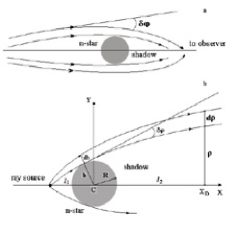
Figure 1: The ray bending and shadow region in the case $l_{1}>>R$ (a); the ray bending and shadow region in the case $l_{1}\geq R$ (b).

Since the value $\xi{\bf m}^{2}/r^{6}$ is small, in order to find the bending angles $\delta\varphi^{*}_{1,2}$ we can use the algorithm (Darwin 1961), well established for calculations of angles of light gravitational bending. The details of calculations of the bending angle $\delta\varphi^{*}_{1}$ in the case of an electromagnetic wave polarized in the $XOY$ plane, and $\delta\varphi^{*}_{2}$ for an electromagnetic wave polarized along the $z$ axis, are presented in Appendix B. For the case, when $b<l_{1}<<l_{2},$ and $l_{2}>>b$ we obtained following relations for the bending angles:

$$\delta\varphi_{1}^{*}=\arctan\left[{bQ_{1}\over\sqrt{Q_{1}^{2}l_{1}^{2}-1}}\right]+{15\pi\eta_{1}\xi{\bf m}^{2}\over 4b^{6}}-$$ (16)

$$-\big{[}1+{15\eta_{1}\xi{\bf m}^{2}\over 4b^{6}}\big{]}\arcsin({1\over Q_{1}l_{1}})-$$

$$-{\eta_{1}\xi{\bf m}^{2}\over 16b^{6}}\big{\{}\sin[4\arcsin({1\over Q_{1}l_{1}})]-16\sin[2\arcsin({1\over Q_{1}l_{1}})]\big{\}},$$

$$\delta\varphi_{2}^{*}=\arctan\left[{bQ_{2}\over\sqrt{Q_{2}^{2}l_{1}^{2}-1}}\right]+{15\pi\eta_{2}\xi{\bf m}^{2}\over 4b^{6}}-$$

$$-\big{[}1+{15\eta_{2}\xi{\bf m}^{2}\over 4b^{6}}\big{]}\arcsin({1\over Q_{2}l_{1}})-$$

$$-{\eta_{2}\xi{\bf m}^{2}\over 16b^{6}}\big{\{}\sin[4\arcsin({1\over Q_{2}l_{1}})]-16\sin[2\arcsin({1\over Q_{2}l_{1}})]\big{\}},$$

where

$$Q_{1}={1\over b}\big{[}1+{2\eta_{1}\xi{\bf m}^{2}\over b^{6}}\big{]},\ \ \ \ Q_{2}={1\over b}\big{[}1+{2\eta_{2}\xi{\bf m}^{2}\over b^{6}}\big{]}.$$

The plus sign in this relation shows, that the magnetic dipole field in the magnetic equator plane effects the electromagnetic waves as a convex lens. To illustrate dependeces (16) in BI and HE theories we plot $\delta\varphi_{1}^{*}$ and $\delta\varphi_{2}^{*}$ versus $b/l_{1}$ for different values $B_{0}/B_{q}$ (Fig. 2 – Fig. 4).

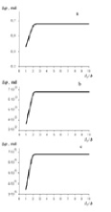
Figure 2: The BI dependence $\delta\varphi$ versus $l_{1}/b$ for different values ${\bf B}^{2}(b)/B_{q}^{2}:$ $(a)\ {\bf B}^{2}(b)/B_{q}^{2}=10^{-2},\ (b)\ {\bf B}^{2}(b)/B_{q}^{2}=10,(c)\ {\bf B}^{2}(b)/B_{q}^{2}=1$ (${\bf B}^{2}(b)$ is the square of magnetic field at the distance $b$ from the neutron star, $\delta\varphi_{1}^{*}=\delta\varphi_{2}^{*}).$

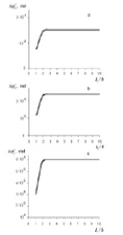
Figure 3: The HE dependence $\delta\varphi_{1}^{*}$ versus $l_{1}/b$ for different values ${\bf B}^{2}(b)/B_{q}^{2}:$ $(a)\ {\bf B}^{2}(b)/B_{q}^{2}=0.25,\ (b)\ {\bf B}^{2}(b)/B_{q}^{2}=0.04,(c)\ {\bf B}^{2}(b)/B_{q}^{2}=0.01$ (${\bf B}^{2}(b)$ is the square of magnetic field at the distance $b$ from the neutron star).

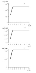
Figure 4: The HE dependence $\delta\varphi_{2}^{*}$ versus $l_{1}/b$ for different values ${\bf B}^{2}(b)/B_{q}^{2}:$ $(a)\ {\bf B}^{2}(b)/B_{q}^{2}=0.25,\ (b)\ {\bf B}^{2}(b)/B_{q}^{2}=0.04,(c)\ {\bf B}^{2}(b)/B_{q}^{2}=0.01$ (${\bf B}^{2}(b)$ is the square of magnetic field at the distance $b$ from the neutron star).

Thus, nonlinear models of vacuum electrodynamics with $\eta_{1}\neq\eta_{2},$ predict different angles of ray bending for electromagnetic waves with different polarization.

It should be noted, that besides the nonlinear electrodynamic bending (16) of electromagnetic rays will also undergo the well known gravitational bending. However, because of the different bending angle dependence on the impact distance $b$ ($1/b$ and $1/b^{2}$ in the case of gravitational bending (Epstein $\&$ Shapiro 1980; Will 1981; Meszaros $\&$ Riffert 1988; Riffert $\&$ Meszaros 1988) and $1/b^{6}$ in the case of nonlinear electrodynamic bending) mathematical processing allows to resolve each of these parts from the observational data if the time dependence of impact distance $b$ is harmonical $b(t)=b_{0}+R_{1}\cos\Omega t.$

4 The effect of gamma-ray flux scattering in the neutron star magnetic field

The nonlinear electrodynamic bending of rays in the magnetic dipole field differs significantly from gravitation bending of these rays. As it is well-known, the ray bending in the Schwarzschild gravitation field occurs in the plane containing this ray and the star center. Thus, gravitation ray bending leads to the increase of electromagnetic flux detected by the instrument located on the other side of gravitation center.

In the general case the nonlinear electrodynamic bending of electromagnetic ray is not planar. It can be discribed as the bending on the series of magnetic force lines, when a ray undergoes bending on every force line in the plane containing the normal to the surface $[{\bf B}_{0}\ {\bf k}]^{2}/k^{2}=const.$ As a result the nonlinear interaction of electromagnetic wave with the dipole magnetic field leads in the general case to the appearing of the ray curvature and twisting.

For a complete and detailed study of the principles of nonlinear electrodynamic lensing, it is necessary to solve Eqs. (12) in the very general case, but not only for rays laying in the neutron star magnetic equator plane. However, to the present time the solution of these equations is unknown. Formulas (16) allow us to study only one particular case of nonlinear electrodynamic lensing, when the ray source is near the neutron star, at the distance $l_{1}\sim R$, and electromagnetic emission is a bunch of rays laying in the small vicinity of magnetic equator plane.

When studying gravitation lensing of light emission, it can usually be assumed that the distance between light source and the gravitating star $l_{1}$ is larger than the star radius $R$. In this case ray bending leads to the abrupt cutting of the field of shadow behind the opaque star (see Fig. 1a). As a result, the light flux detected at the large distance will be much larger than in the case of gravitating center absence (the effect of gravitational lensing).

The sources of gamma-rays are located mainly not far, or according to some models (Harding, 2000), even near the pulsar’s or magnetar’s surface: $l_{1}\sim R$. Thus, even with account for the gravitational and nonlinear electromagnetic bending of gamma-rays, we should assume the existence of some shadow cone behind the neutron star, where gamma-rays never penetrate (see Fig. 1b).

The main condition of the existence of such cone is the non-equality: $\delta\varphi_{max}<\arcsin(R/l_{1}).$ Let us consider this case in details.

We will assume, that a magnetized neutron star is located in the coordinate center, the gamma ray source is placed in the $XOY$ plane at the distance of $l_{1}$ from the neutron star (left panel of Fig. 1b) and the spacecraft carrying the gamma ray detector is located at a large distance from the star, at the point $x_{D}=l_{2}>>l_{1},\ y_{D}=\rho.$ Let us calculate the value of gamma-ray flux $I_{out}$ detected by the presence of gravitation and nonlinear electrodynamic bending of rays.

Let us assume, that in the case of the absence of such bending, the detector will measure the energy flux $I_{0}=A/\sigma[\rho^{2}+(l_{1}+l_{2})^{2}],$ where $\sigma$ is the value of gamma-ray beam solid angle, $A$ is some constant characterizing the gamma-ray source intensity.

It is quite appropriate to chose the sector of a ring of radius, $b,$ width, $db$ and angle opening $\delta\theta<<1$ as the input aperture. This aperture area will be equal to: $S_{in}=bdb\delta\theta.$

In the input aperture plane the gamma-ray flux $I_{in}$ will be: $I_{in}=A/\sigma[l_{1}^{2}-R^{2}]=I_{0}[\rho^{2}+(l_{1}+l_{2})^{2}]/[l_{1}^{2}-R^{2}].$ Since in the field of the magnetic equator it is possible to consider the gravitational and nonlinear electrodynamic bending of rays as occurring approximately in the planes containing the neutron star center, the output aperture can also be presented as the sector of a ring of radius, $\rho$, width, $d\rho.$, and angle opening $\delta\theta.$ Thus the output aperture area will be equal to: $S_{out}=\rho d\rho\delta\theta.$

Since the energy value transferred per unit time along the bunch of rays does not depend on the distance, then from the equality $I_{in}S_{in}=I_{out}S_{out}$ we obtain:

$$I_{out}={I_{0}[\rho^{2}+(l_{1}+l_{2})^{2}]\over(l_{1}^{2}-R^{2})}{b\over\rho}{db\over d\rho}.$$ (17)

In this relation values $\rho$ and $b$ are not independent, but are connected by the equation, which can easily be obtained from geometrical consideration (see Fig. 1b):

$$\rho=b\cos\alpha_{0}+\big{[}b\sin\alpha_{0}+l_{2}\big{]}tg\Big{(}\alpha_{0}-{2r_{g}\over b}-\delta\varphi_{1,2}^{*}\Big{)},$$ (18)

where $\alpha_{0}=\arcsin(b/l_{1}),$ $r_{g}$ is the Schwarzschild radius of neutron star, and $\delta\varphi^{*}_{1,2}$ is defined by espression (16).

This equation is transcendental relatively to the impact parameter $b.$ Its analytical approximate solution can be obtained only under a large number of restrictions on the parameters contained in it. In particular, if $R\sim 10^{2}$ km, $l_{1}\sim 10^{4}$ km, $r_{g}\sim 0.2$ km, $l_{2}\sim 10^{17}$km, $\delta\varphi^{*}_{1,2}<10^{-2},$ then is transcendental equation (18) by $2R\geq b\geq R$ can be approximate by algebraic equation of the 7th order relatively to the impact parameter $b:$

$$\rho=l_{2}\Big{[}{b\over l_{1}}-{2r_{g}\over b}-{15\pi\xi\eta_{1,2}|{\bf m}|^{2}\over 4b^{6}}\Big{]}.$$

Since $b\geq R,$ and $R/l_{1}\sim\ 10^{-2},$ the last two terms in the squared brackets give the small correction to $b/l_{1},$ which decreases with the increasing $b.$ As a result, the approximate solution of this equation can be written as:

$$b={l_{1}\rho\over l_{2}}\Big{\{}1+{l_{2}\over\rho}\Big{[}{2r_{g}l_{2}\over l_{1}\rho}+{15\pi\xi\eta_{1,2}|{\bf m}|^{2}l_{2}^{6}\over 4l_{1}^{6}\rho^{6}}+O\Big{(}{r_{g}^{2}l_{2}^{2}\over l_{1}^{2}\rho^{2}}\Big{)}\Big{]}\Big{\}},$$ (19)

and this solution is valid only by variation of $\rho$ within the limits: $2l_{2}R/l_{1}>\rho>l_{2}[R/l_{1}-2r_{g}/R-15\pi\xi\eta_{1,2}|{\bf m}|^{2}/(4R^{6})].$

Substituting expression (19) in the equality (17), we then obtain, that in this field of variation of $\rho$ the detected gamma-ray flux will be equal:

$$I_{out}=I_{0}\Big{[}1-{75\pi\xi\eta_{1,2}|{\bf m}|^{2}l_{2}^{7}\over 4l_{1}^{6}\rho^{7}}+O\Big{(}{r_{g}^{2}l_{2}^{3}\over l_{1}^{2}\rho^{3}}\Big{)}\Big{]}<I_{0}.$$ (20)

Thus, gravitation and nonlinear electrodynamic bending of gamma-rays leads to a decrease of the detected flux in the considered part of space. It is caused by consideration, that in the absence of the ray bending the illuminated area $\rho\geq Rl_{2}/l_{1}$ is less than illuminated area $\rho\geq l_{2}[R/l_{1}-2r_{g}/R-15\pi\xi\eta_{1,2}|{\bf m}|^{2}/(4R^{6})]$ in the presence of bending. As a result of the ray bending, part of the gamma-ray energy flux is transferred from the field of space $\rho\geq Rl_{2}/l_{1}$ to the field of space bounded by the conic surfaces $\rho=Rl_{2}/l_{1}$ and $\rho=l_{2}[R/l_{1}-2r_{g}/R-15\pi\xi\eta_{1,2}|{\bf m}|^{2}/(4R^{6})],$ thus decreasing the flux of energy outside the cone $\rho\geq Rl_{2}/l_{1}.$

We will make some estimates. If we use the above presented numerical values of $R,l_{1},r_{g},l_{2}$ and if to assume that in the case of some gamma-ray pulsars near the neutron star surface $B_{0}=2\cdot 10^{13}\ G,$ (Thompson 2000) we obtain, that relative value $(I_{0}-I_{out})/I_{0}$ changes from $10^{-2}$ at $\rho=Rl_{2}/l_{1}\sim 10^{15}$ km to $10^{-4}$ at $\rho=2Rl_{2}/l_{1}\sim 2\cdot 10^{15}$ km.

Due to the larger magnetic field $B_{0}\sim\cdot 10^{15}-10^{16}\ G,$ (Zhang $\&$ Harding 2000; Duncan $\&$ Thompson 1992; Thompson $\&$ Duncan 1995, 1996) in the case of a magnetar this value will change in wider boundaries. However, the correct estimates in post-Maxwellian approximation can be made only in the frame of the BI electrodynamics, since in the HE theory, if the magnetic field is greater than the $B_{q}$ value, the Lagrangian should be changed drastically, because it sh ould contain logarithmic terms.

5 Analysis of x-ray and gamma-ray astronomy technique applications for observing nonlinear electrodynamic effects

The modern accuracy of gamma ray flux parameter measurements provided by the use of extra-Terrestrial techniques is much worse than the accuracy of measurements of similar parameters in the optical range (Boyarchuk et al. 1999). However, due to the opacity of the strongly magnetized neutron star magnetosphere to the optical emission, X-rays and gamma rays give the unique possibility to research for nonlinear electrodynamic effects in the strong magnetic field of a neutron star.

5.1 The effect of gamma-ray flux dispersion

Taking into account the capabilities of modern X-ray and gamma ray space observatories discussed in the Introduction, we will analyze, which of the above mentioned effects can be observed using space astronomy techniques.

In the case, when the distance $l_{1}$ between the gamma ray source and the neutron star is comparable with the neutron star radius, the energy flux (20) is close to one even for the impact distances comparable to the star radius. Thus, the rays which underwent significant nonlinear electromagnetic influence from the neutron star magnetic field can be weakly dispersed, and as a result their intensity at the point of observation will be sufficient for detection.

Let us estimate the magnitudes of these effects. However, first of all it is necessary to make the following clarification. All the above discussed effects depend not only on the magnetic field value, but also on the choice of the model nonlinear vacuum electrodynamics (since transition from one model to another changes the value of post-Maxwell parameters $\eta_{1}$ and $\eta_{2}$). At present it is impossible to say, which value of these parameters is agrees with observational data.

It is necessary to note, that in the HE nonlinear electrodynamics (Ritus 1986) the expansion parameter is $p=({\bf B}/B_{q})^{2}.$ By $B=2\cdot 10^{13}$ G this parameter is equal to $p=0.2$ and post-Maxwellian expansion (5) of QED still can be used for estimation of nonlinear effects values.

Thus, when making the estimates we will take into account the most well known models of nonlinear vacuum electrodynamics, such as the BI electrodynamics and the nonlinear electrodynamics, which is the direct consequence of quantum electrodynamics. According to these theories the post-Maxwell corrections to the Lagrangian of nonlinear electrodynamics are about $\sim 10^{-4}{\bf B}^{2}/B_{q}^{2}.$

However, it is necessary to note, that these estimates are quite conditional, and should be considered as estimates of concrete theories. It may be, that some other theory is more adequate to nature, and will give other estimates of the studied nonlinear electrodynamic effect values in the discussed experiments. During the space experiments it is necessary to search for and measure record all the above mentioned effects in order to obtain the values of post-Maxwell parameters $\eta_{1}$ and $\eta_{2}$ from the results of observational data processing. Thus, the purpose of astrophysical observations is not only the testing the predictions of one or another nonlinear vacuum electrodynamics model, but also what is more important the measuring of parameters $\eta_{1}$ and $\eta_{2}$.

Using equalities (16), it is not difficult to obtain, that the maximum value of the nonlinear electrodynamic bending angle of gamma-rays in the magnetic field of a pulsar with $B=2\cdot 10^{13}$ G is about $\delta\varphi^{*}\sim 2.1\cdot 10^{-4}$ rad $\approx 40$ arcsec according to the quantum electrodynamics predictions and $\delta\varphi^{*}\sim 1.4\cdot 10^{-5}$ rad $\approx 2.8$ arcsec according to the BI electrodynamics.

In the field of gamma-ray pulsar or magnetar with $B\sim 10^{16}$G the maximum value of this angle increases: $\delta\varphi^{*}\sim 3.5$ rad $\approx 200^{\circ}$ according to the BI electrodynamics.

It is necessary to note that, the magnetic field of real neutron stars is most certainly not dipolar (Feroci et al. 2001). In the case of a non dipolar field the effective volume of nonlinear electrodynamics interaction, will be smaller in comparison with the case of a dipolar field. Thus, the gamma-ray bending will be less clearly pronounced. However, the above obtained estimates made for the dipole field can be used for model quantitative evaluations of nonlinear electrodynamics effects.

It is necessary to note that the obtained values characterize deflection angles at the source. At the point of observation possible deflection of a ray will be determined by the attitude $\delta b/l_{2},$ were $\delta b$ is the variation of the impact parameter of a ray because of the proper move of the source and $l_{2}$ is the distance from the source to observer. For typical values $l_{2}=10^{17}$ km (3 kps), $\delta b=10^{2}$ km, $\delta b/l_{2}\sim 3.4\cdot 10^{-12}$ arcsec that is beyond any measurable limits now. The only nonlinear electrodynamics effect, which can be measured principally, is the effect of gamma ray flux dispersion by the neutron star magnetic field. It follows from equation (20) that flux attenuation coefficient depends on the impact parameter $b$ as well as on the ray bending angle. Thus, studying this effect we could also obtain information on the nonlinear electrodynamics bending of a ray in the source.

The effect of gamma ray flux dispersion can be interpreted more accurately, if the neutron star and the gamma ray source are moving relatively each other with periodical time dependence of their mutual location. As our estimates show, the limits of the flux attenuation coefficient value in this case are very wide. Hence, in the case of a rotating neutron star, if gamma rays are emitted in its vicinity, we will have periodic variations of the impact parameter which lead to the periodic variations of the flux attenuation coefficient. Such variations will efficiently modulate the mean light curve, which can be detected by the outside observer. Under certain conditions the same effect in the orbital light curves could be observed in the case of pulsars in binary systems. However, the presence of accreting matter can lead to some difficulties in resolving the pure nonlinear electrodynamic effect from the mean orbital light curves.

5.2 The effect of birefringence

The main qualitative difference in the predictions of different nonlinear electrodynamics theories, which can be observed in the considered astrophysical conditions, is the absence of birefringence in the BI theory. According to the HE theory vacuum birefringence effects the polarization of the emitted photons as well as the radiative opacity of the near neutron star medium. Such effects leads to a signature in the emission spectra. However, for X-ray frequencies and pulsar magnetic fields to be quite pronounced this effect requires rather high plasma density ($10^{23}$ cm^-3) (Meszaros $\&$ Ventura 1979), which can take place in some accretion powered pulsars. In the case of individual magnetic neutron stars (gamma-ray pulsars and magnetars) the magnetosphere is quite transparent for hard emission. The main effect, which has influence on the propagation of emitted photons, is absorption by pair production in a strong magnetic field. This suppresses the radiation above about 1 MeV and effects the gamma ray beaming (Riffert et al. 1989).

As for X- ray frequencies in the case of pulsars with poor magnetosphere we suppose, that the only observable difference between predictions of BI and HE theories is that according to the first theory the nonlinear electrodynamic bending angle in the dipole magnetic field of a neutron star and consequently the flux attenuation coefficient will be the same for any polarization of electromagnetic waves. In the HE theory $\eta_{1}\neq\eta_{2}$ as well as the nonlinear electromagnetic bending angle and consequently the flux attenuation coefficient depend on the electromagnetic wave polarization.

Thus, this theory predicts that if the gamma-ray source moves periodically relatively to the neutron star (i.e. in the case of rotating neutron star or pulsar in binary system) we will obtain different mean light curves for emitted electromagnetic waves with perpendicular mutual linear polarization.

6 Discussion

Although the observation of the manifestations of the nonlinear electrodynamics effects in astrophysical objects requires special conditions, in principle, they can be observed. The main astrophysical objects, where the nonlinear electrodynamic effects can be revealed more clearly, are certain kinds of gamma-ray pulsars and magnetars. These effects can be manifested as some peculiarities in the form of their hard emission pulsation.

The typical luminosity of magnetars and certain kinds of rotation-powered pulsars in hard emission is about $10^{34}-10^{36}$ erg s^-1 (Mereghetti 2000). For example, the sensitivity level of the Chandra instruments for $10^{4}$ s exposure corresponds to the luminosity of galactic objects $\sim 10^{30}-10^{31}$ erg s^-1 ( Garcia et al. 2001). Hence, for the exposure time of about 1 s Chandra permits to obtain the mean light curve of a source with the luminosity of $\sim 10^{32}-10^{33}$ erg s^-1, this is about two order lower than the typical luminosity of such magnetar-candidate sources as AXPs or SGRs.

The imaging mode of an instruments is not necessary for obtaining the mean light curve, because for most of these objects (soft gamma-ray repeaters, anomalous X- ray pulsars, etc) the pulsation period is known. However, the detector outputs should be folded over the maximum possible time of continuous exposure with that known period. For example, we can take $10^{5}s$ as the exposure time of a given source, thus according to the announced sensitivity for TeCd detector of the INTEGRAL IBIS instrument (Winkler 2001) we obtain the minimum detectable intensity of periodic processes (at $8\sigma$ level), which is about 1 mCrab. This estimate permits to obtain the mean curve of pulsation for a source like a SGR even in its quiescent state. Since the number of known magnetar-like sources is not large, the inspection of most of them during the mission will be quite justified.

Measurements of the bending angle in the source need observations of at least the proper orbital motion of the pulsar, which is not accessible by currently operating instruments.

The additional group of effects may be connected with such objects as accretion-powered binary X-ray pulsars and, possibly other kinds of tight binaries containing magnetic neutron stars. As it was mentioned above, the objects with most suitable conditions for nonlinear electrodynamics effects are binary systems with underfilled Roche lobe supergiants as an optical companion. The value of the orbital period provides the necessary time for continuous observations of these sources. Because most of pulsar systems with underfilled Roche lobe optical companion are characterized by large orbital periods (4U1538-522, 3.73 d; 4U1907+097, 8.38 d; 1E1145.1-614, 5.648 d; Vela X-1, 8.965 d) (Bieldsten et al. 1997), rather long exposures are necessary to obtain detailed mean orbital light curves. The existense of certain non-typical forms can indicate the presence of nonlinear electrodynamic effects in such objects.

Appendix A Eikonal equation

Using Lagrangian (9), it is not difficult to obtain the expansion of vectors $\bf D$ and $\bf H$ onto degrees $\xi$ with accuracy up to $\xi^{2}$ inclusive:

$${\bf D}={\bf E}+\xi\{2\eta_{1}({\bf E}^{2}-{\bf B}^{2}){\bf E}+4\eta_{2}({\bf B\cdot E}){\bf B}\}+$$ (21)

$$+\xi^{2}\{3\eta_{3}({\bf E}^{2}-{\bf B}^{2})^{2}{\bf E}+\eta_{4}({\bf B\cdot E})^{2}{\bf E}+$$

$$+\eta_{4}({\bf E}^{2}-{\bf B}^{2})({\bf B\cdot E}){\bf B}\}\},$$

$${\bf H}={\bf B}+\xi\{2\eta_{1}({\bf E}^{2}-{\bf B}^{2}){\bf B}-4\eta_{2}({\bf B\cdot E}){\bf E}\}+$$

$$+\xi^{2}\{3\eta_{3}({\bf E}^{2}-{\bf B}^{2})^{2}{\bf B}+\eta_{4}({\bf B\cdot E})^{2}{\bf B}-$$

$$-\eta_{4}({\bf E}^{2}-{\bf B}^{2})({\bf B\cdot E}){\bf E}\}.$$

Under the assumption of a ”weak” plane electromagnetic wave (8) with the use of an approximation linear in vectors $\bf b$ and $\bf e$, we can obtain from relation (A1) and equations (1) a uniform system of three linear algebraic equations relatively to three $\bf e$ components:

$$\Pi^{\alpha\beta}e_{\beta}=0,$$ (22)

where

$$\Pi^{\alpha\beta}=A_{0}\{k^{\alpha}k^{\beta}+({\omega^{2}\over c^{2}}-{\bf k}^{2})\delta^{\alpha\beta}\}+$$

$$+A_{1}N_{B}^{\alpha}N_{B}^{\beta}+A_{2}{\omega^{2}\over c^{2}}B_{0}^{\alpha}B_{0}^{\beta},$$

and for more compact record we introduce the following notations:

$$A_{0}=1-2\eta_{1}\xi{\bf B}_{0}^{2}+3\eta_{3}\xi^{2}{\bf B}_{0}^{4},\ \ \ A_{1}=4\eta_{1}\xi-12\eta_{3}\xi^{2}{\bf B}_{0}^{2},$$

$$A_{2}=4\eta_{2}\xi-\eta_{4}\xi^{2}{\bf B}_{0}^{2},\ \ \ \ {\bf N}_{B}=[{\bf k\times B}_{0}].$$

For the existence of nontrivial solutions of the equations system (A2) it is necessary, that $det||\Pi^{\alpha\beta}||=0.$ The determinant of tensor $\Pi^{\alpha\beta}$ can be calculated in the most simple way, if we use the formulas of tensor algebra verified in the work of Denisova $\&$ Mehta (1997).

The condition of equality to zero of the second order tensor determinant in three-dimensional Euclidean space $\Pi^{\alpha\beta}$ can be rewritten using these formulas in the form:

$$2\Pi_{(3)}-3\Pi_{(1)}\Pi_{(2)}+\Pi_{(1)}^{3}=0,$$

where

$$\Pi_{(N)}=\Pi_{\alpha_{1}\beta_{1}}\delta_{\beta_{1}\alpha_{2}}\Pi_{\alpha_{2}\beta_{2}}\delta_{\beta_{2}\alpha_{3}}\dots\Pi_{\alpha_{N}\beta_{N}}\delta_{\beta_{N}\alpha_{1}}.$$

To compose the tensor’s degrees $\Pi^{\alpha\beta},$ after the reduction by $\omega^{2}A_{0}/c^{2}$ we obtain the following dispersion equation:

$${\omega^{4}\over c^{4}}\Big{\{}A_{2}A_{0}{\bf B}_{0}^{2}+A_{0}^{2}\Big{\}}+{\omega^{2}\over c^{2}}\Big{\{}A_{4}[{\bf k\times B}_{0}]^{2}{\bf B}_{0}^{2}-$$ (23)

$$-A_{2}A_{0}{\bf B}_{0}^{2}{\bf k}^{2}-2A_{0}^{2}{\bf k}^{2}+A_{1}A_{0}[{\bf k\times B}_{0}]^{2}-$$

$$-A_{2}A_{0}({\bf k\times B}_{0})^{2}\Big{\}}+A_{0}^{2}{\bf k}^{4}-A_{1}A_{0}{\bf k}^{2}[{\bf k\times B}_{0}]^{2}+$$

$$+A_{2}A_{0}{\bf k}^{2}({\bf k\cdot B}_{0})^{2}-A_{4}[{\bf k\times B}_{0}]^{2}({\bf k\cdot B}_{0})^{2}=0,$$

where $A_{4}=A_{1}A_{2}-A_{3}^{2}.$

We will find the solution $\omega=\omega({\bf k})$ of this equation as the expansion onto degrees $\xi,$ similar to the expansion of the Lagrangian (9):

$$\omega=ck[1+\xi F+\xi^{2}U],$$ (24)

where $F$ and $U$ are unknown functions.

Let us substitute now this expansion into equation (A3). Because the Lagrangian (9) is written with accuracy up to terms proportional $\xi^{2}$ inclusive, after calculations we can neglect the insignificant terms $\xi^{3}.$ As a result we obtain a relation, which has the form of expansion in degrees $\xi,$ in view of its complication we will not write it here.

To make equal to zero the coefficients of this expansion in degrees $\xi,$ we obtain the equation allowing to determine the unknown functions $F$ and $U.$ In the lowest approximation we have:

$$\{Fk^{2}+2\eta_{1}[{\bf k\times B}_{0}]^{2}\}\{Fk^{2}+2\eta_{2}[{\bf k\times B}_{0}]^{2}\}=0.$$

To resolve this equations relative to $F$ and substitute it by (A4), and obtain the dispersion equations (10).

Appendix B Calculation of the ray bending angle

Differentiating the eikonal (15) with respect to $\alpha$ and making it equal to the constant $\beta,$ we obtain equation for a ray $\varphi=\varphi(r):$

$$\varphi=\beta+\alpha\int\limits^{r}{dr\over r^{2}\sqrt{{{\cal E}_{0}^{2}\over c^{2}}\big{[}1+{4\eta_{1}\xi{\bf m}^{2}\over r^{6}}\big{]}-{\alpha^{2}\over r^{2}}}}.$$ (25)

If we denote the source emission frequency as $\omega_{0}$, then the constant ${\cal E}_{0}=\omega_{0},$ and $\alpha=-\omega_{0}b/c,$ where $b$ - is the impact distance of the ray.

As a result expression (B1) becomes:

$$\varphi=\beta+b\int\limits^{r}{dr\over r^{2}\sqrt{1+{4\eta_{1}\xi{\bf m}^{2}\over r^{6}}-{b^{2}\over r^{2}}}}.$$ (26)

The integral in the right-hand part of this equality can be expressed through elliptical functions. However, it is more favorable for our purposes to find another approach. Let us differentiate the equality (B2) with respect to $\varphi$ and then to raise it into the second-order power:

$$\Big{(}{dr\over d\varphi}\Big{)}^{2}={r^{4}\over b^{2}}\Big{[}1+{4\eta_{1}\xi{\bf m}^{2}\over r^{6}}-{b^{2}\over r^{2}}\Big{]}.$$ (27)

To find the solution of this equation we will use the well known Darwin method (1961). First of all, we will introduce the subsidiary variable $u=1/r.$ The equation (B3) becomes:

$$\Big{(}{du\over d\varphi}\Big{)}^{2}={1\over b^{2}}\big{[}1+4\eta_{1}\xi{\bf m}^{2}u^{6}-b^{2}u^{2}\big{]}.$$ (28)

We will find the solution of this equation in the form, as

$$u=A+Q_{1}\sin\Psi(\varphi),$$ (29)

where $A$ and $Q_{1}$ are constants.

Substituting expression (B5) into equation (B4) and restricting ourselves by the accuracy linear in the small parameter $\eta_{1}\xi{\bf m}^{2}u^{6},$ we obtain:

$$A=0,\ Q_{1}={1\over b}\big{[}1+{2\eta_{1}\xi{\bf m}^{2}\over b^{6}}\big{]},$$

and function $\Psi(\varphi)$ with acceptable accuracy should satisfy equation

$${d\Psi(\varphi)\over d\varphi}=1-{2\eta_{1}\xi{\bf m}^{2}\over b^{6}}\big{[}3-3\cos^{2}\varphi+\cos^{4}\varphi\big{]}.$$

The solution of this equation is:

$$\Psi(\varphi)=\varphi-\varphi_{0}-{\eta_{1}\xi{\bf m}^{2}\over 16b^{6}}\big{[}60\varphi-16\sin 2\varphi+\sin 4\varphi\big{]}.$$

In the case, when the gamma-ray source is located at a limited distance from a neutron star or even in its nearest vicinity let us consider that this source is at the point $r=l_{1},\ \varphi=\pi.$ Then for a ray with impact distance $b$ the solution of equation (B4) can be represented as:

$$u={1\over r}=Q_{1}\sin\big{\{}\varphi-\varphi_{0}-{\eta_{1}\xi{\bf m}^{2}\over 16b^{6}}\big{[}60\varphi-16\sin 2\varphi+\sin 4\varphi\big{]}\big{\}}.$$

Because this ray should pass through the point $r=l_{1},\ \varphi=\pi,$ the integration constant $\varphi_{0}$ is more complicated in comparison with expression (B6):

$$\varphi_{0}=-{15\pi\eta_{1}\xi{\bf m}^{2}\over 4b^{6}}+\arcsin({1\over Q_{1}l_{1}}).$$

The bending angle $\delta\varphi_{1}^{*}$ of a ray after its passing through the neutron star magnetic field will be equal to: $\delta\varphi_{1}^{*}=\varphi_{1}-\varphi_{D},$ where $\varphi_{1}$ is the angle of a ray inclination to the $X$ axis at the point $r=l_{1},\ \varphi=\pi,$ and $\varphi_{D}$ is the angle of the detected ray inclination to the $X$ axis.

Since in the considered case $l_{2}>>l_{1},$ the $\varphi_{D}$ angle can be determined from the condition: $u(\varphi_{D})=1/l_{2}\approx 0.$ It follows from this, that

$$\varphi_{D}=-{15\pi\eta_{1}\xi{\bf m}^{2}\over 4b^{6}}+\Big{[}1+{15\eta_{1}\xi{\bf m}^{2}\over 4b^{6}}\Big{]}\arcsin({1\over Q_{1}l_{1}})+$$

$$+{\eta_{1}\xi{\bf m}^{2}\over 16b^{6}}\big{\{}\sin[4\arcsin({1\over Q_{1}l_{1}})]-16\sin[2\arcsin({1\over Q_{1}l_{1}})]\big{\}}.$$

As it is well known, the tangens of $\varphi_{1}$ inclination angle at the point $r=l_{1},\ \varphi=\pi,$ is equal to the derivative $dy/dx$ at this point:

$$tg(\varphi_{1})={dy\over dx}(r=l_{1},\varphi=\pi)=$$

$$={r^{\prime}\sin\ \varphi+r\cos\ \varphi\over r^{\prime}\cos\ \varphi-r\sin\ \varphi}=-{1\over l_{1}u^{\prime}}(\varphi=\pi),$$

where the apostrophe denotes the derivative over $\varphi.$

In the first approximation in the small parameter $\xi{\bf m}^{2}/b^{6}$ it can be obtained from this:

$$\varphi_{1}=\arctan\left[{bQ_{1}\over\sqrt{Q_{1}^{2}l_{1}^{2}-1}}\right].$$

As a result we obtain the formula (16) for the bending angle $\delta\varphi_{1}^{*}$ of a ray.

References

- (1) Alexandrov, E.B., Anselm, A.A., Moskalev, A.N. 1985, JETP, 62, 680
- (2) Bakalov, D. et al. Quantum Semiclass. Opt. 1998, 10, 239
- (3) Bildsten, L., et al. 1997 ApJS 113, 367
- (4) Born, M., Infeld, L. 1934, Proc. Roy. Soc., A144, 425
- (5) Boyarchuk, A.A., Bagrov, A,V,, Mikisha, A.M,, Rykhlova, L.V., Smirnov, M.A., Tokovinin, A.A., Etsin, I.S. 1999, Cosmic Research, 37, 3
- (6) Brner, G., Meszaros, P. 1979 AA 77, 178
- (7) Burke D.L. et al. 1997, Rhys. Rev. Lett. 79, 1626
- (8) Bussard et al. 1986, Phys. Rev. D34, 440
- (9) Cash, W.C., White, N., Joy, M.K. 2000 Proc. SPIE 4012, X-Ray Optics Instruments and Missions, eds. J.E. Trumper, B. Aschenbach, 258
- (10) Cecotti, S. Ferrara, S. 1987 Phys. Lett., B187, 335
- (11) CXC, Chandra MSFC, and Chandra IPI Teams 2000, Chandra Proposers Observatory Guide (POG) Electron. Version 2.0
- (12) Darwin, C. 1961 Proc. Roy. Soc. London A263, 39
- (13) De Lorenci, V.A., Figueiredo, N., Fliche, H.H., Novello, M. 2001 AA 369, 690
- (14) Denisov, V.I. 2000, Phys. Rev., D61, 036004
- (15) Denisov, V.I. 2000, Journal of Optics, A2, 372
- (16) Denisov, V.I., Denisova, I. P. 2001, Optics and Spectroskopy, 90, 282
- (17) Denisov, V.I., Denisova, I. P. 2001, Optics and Spectroskopy, 90, 928
- (18) Denisov, V.I., Denisova, I. P. 2001, Doklady Physics, 46, 377
- (19) Denisov, V.I., Denisova, I. P. 2001, Theoretical and Mathematical Physics, 129, 1421
- (20) Denisov, V.I., Denisova, I. P. Svertilov, S.I. 2001, Doklady Physics, 46, 705
- (21) Denisov, V.I., Kravtsov, N.V., Lariontsev, E.G., Pinchouk, V.B., Zubrilo, A.A. 2000, Moscow University Phys. Bull, 5, 51
- (22) Denisov, V.I., Denisova, I.P., Krivchenkov, I.V. 2002, JETP, 122, 227
- (23) Denisova, I.P., Mehta, B.V. 1997, Gen. Relat. Gravit., 29, 583
- (24) Di Cocco, G., et al. 1997 in Proc. 25th ICRC 5, 25th International Cosmic Ray Conference, eds. M.S. Potgieter, B.C. raubenheimer, D.J. Van Der Walt (Potchefstroom: Space Research Unit, Department of Physics, Potchefstroomse Universiteit), 33
- (25) Duncan, R.C., Thomson, C., 1992 ApJ 392, L9
- (26) Epstein, R., Shapiro, I.I, 1980, Phys. Rev., D22, 2947
- (27) Feroci, M., Hurley, K., Duncan, R.C., Thompson, C. 2001 ApJ 549, 1021.
- (28) Gal’tsov, D.V., Nikitina, N. S., 1983, Sov. Phys.–JETP, 57 705.
- (29) Garcia, M.R., McClintock, J.E., Narayan, R., Callanan, P., Murray, S.S. 2001 ApJ 553, L476
- (30) Gehrels, N., et al., 1997 ESA SP-382, 587
- (31) Ginzburg, V.L. 1987, Theoretical Physics and Astrophysics, (Moscow: Nauka)
- (32) Harding A.K. 2000, Astro-ph/0012268
- (33) HEASARC 2001, High Energy Astrophysics Science Archive Research Center, A Portable Mission Count Rate Simulator (W3PIMMS), Electron. Version 3.1c
- (34) Heisenberg, W., Euler, H. 1936, Z. Phys., 26, 714
- (35) Landau, L.D., Lifshitz, E.M. 1984, Field Theory, (Oxford: Pergamon)
- (36) Lasota, J.-P. 2000 AA 360, 575L
- (37) Meszaros, P. 1992, High Energy Radiation from Magnetized Neutron Stars, (Chicago: Univ. of Chicago Press)
- (38) Meszaros, P. et al. 1980 ApJ 238, 1066
- (39) Meszaros, P., Bonazzola, S. 1981 ApJ, 251, 695
- (40) Meszaros, P., Riffert, H. 1988 ApJ, 327, 712
- (41) Meszaros, P., Ventura, J. 1978, Phys. Rev. Lett., 41, 1544
- (42) Meszaros, P., Ventura, J. 1979, Phys. Rev., D19, 3565
- (43) Parmar, A.N., et al. 1999 astro-ph9911494
- (44) Rikken, G.L.J.A., Rizzo, C. 2000, Phys. Rev., A63, 012107
- (45) Ritus, V.I., 1986, Proceedings of P.N. Lebedev Physical Institute, 168, 5
- (46) Rosanov, N.N. 1993, JETP, 76, 991
- (47) Riffert, H., Meszaros, P. 1988 ApJ, 325, 207
- (48) Sutherland, W. et al. 1996 in Proc. of the 1st Intern. Workshop on the Identification of Dark Matter, ed. N.J.C. Spooner (Singapore: World Sci.), 200
- (49) Thomson, C, Duncan, R.C. 1995 MNRAS 275, 255
- (50) Thomson, C, Duncan, R.C. 1996 ApJ 473, 322
- (51) Thomson, D.J. 2000 Adv. Space Res. 25, 659
- (52) Van Spreybroeck, L., Jerius, D., Edgar R.J., Gaetz T.J., Zhao., P., Reid P.B., 1997 Proc. SPIE 3113, 98
- (53) Ventura, J. et al., 1979 ApJL 233, L125
- (54) Weaver, K.A., White, N.E., Tananbaum, H. 2000 HEAD 32, 2003W
- (55) White, N.E., Tananbaum, H. 2000 IAUS 195, 61W
- (56) Will, C. 1981, Theory and Experiment in Gravitational Physics (Cambrige: Cambrige University Press)
- (57) Winkler, C. 1999 Ap. Lett. Comm. 39, 361
- (58) Winkler, C. 2001 astro-ph0102007
- (59) Zhang, B., Harding, A.K. 2000 ApJ 535, L51