First Results from the Arcminute Cosmology Bolometer Array Receiver

Abstract

We review the first science results from the Arcminute Cosmology Bolometer Array Receiver (Acbar); a multifrequency millimeter-wave receiver optimized for observations of the Cosmic Microwave Background (CMB) and the Sunyaev-Zel’dovich (SZ) effect in clusters of galaxies. Acbar was installed on the 2 m Viper telescope at the South Pole in January 2001 and the results presented here incorporate data through July 2002. We present the power spectrum of the CMB at 150 GHz over the range $\ell=150-3000$ measured by Acbar as well as estimates for the values of the cosmological parameters within the context of $\Lambda$CDM models. We find that the inclusion of $\Omega_{\Lambda}$ greatly improves the fit to the power spectrum. We also observe a slight excess of small-scale anisotropy at 150 GHz; if interpreted as power from the SZ effect of unresolved clusters, the measured signal is consistent with CBI and BIMA within the context of the SZ power spectrum models tested.

1 Introduction

In this proceedings we review the first science results from the Acbar experiment. We present an overview of the receiver, telescope, and site in §2. Our observing technique is described in §3. The map making technique and power spectrum estimation are described in §4. We discuss systematic tests, including a check on foreground contamination, in §5. Estimation of cosmological parameters is presented in §6 and we discuss the results in §7. Further details of the Acbar power spectrum and cosmological parameter extraction are presented in Kuo et al. (2002) and Goldstein et al. (2002), respectively. Due to journal space constraints, we refer the reader to associated papers on Acbar pointed SZ cluster observations (Romer et al. 2003) and blind cluster survey (Runyan et al. 2003b).

2 Instrument and Telescope

The Arcminute Cosmology Bolometer Array Receiver (Acbar) is a 16 pixel, millimeter wavelength, 240 mK bolometer array and is described in detail in Runyan et al. (2003a). The instrument was designed to couple to the existing Viper telescope at the South Pole to produce high resolution maps of the CMB sky with high signal-to-noise.

Acbar is configurable to observe simultaneously at 150, 220, 280 and 350 GHz with bandwidths of 31, 31, 48, and 24 GHz, respectively. In 2001 Acbar had four feeds at each of the four observing frequencies. In 2002 we replaced the 350 GHz feeds with an additional row of 150 GHz feeds because of the superior noise performance at 150 GHz. Acbar makes use of extremely sensitive microlithographed spider-web bolometers developed at JPL for the Planck satellite mission (Turner et al. 2001). These detectors achieve background photon limited performance in Acbar. In 2002 the 150 GHz channels had an average $NET_{RJ}$ sensitivity of $\sim 200~{}\mu{\rm K}\sqrt{s}$. The focal plane is arranged in a $4\times 4$ grid with a spacing of $\sim 16^{\prime}$ between beam centers on the sky.

The Viper telescope is a 2 m off-axis Gregorian telescope designed specifically for observations of CMB anisotropy. The primary is surrounded by a 0.5 m skirt to reflect spillover to the sky. The entire telescope is enclosed in a large conical ground shield to block emission from elevations below $\sim 25^{\circ}$; one section lowers to allow observations of low-elevation sources such as planets. A chopping flat at the image of the primary formed by the secondary sweeps the beams $\sim 3^{\circ}$ in azimuth in a fraction of a second.

The combination of large chop ($\sim 3^{\circ}$) and small beam sizes ($\sim 4-5^{\prime}$ FWHM Gaussians) makes Acbar sensitive to a wide range of angular scales ($150<\ell<3000$), with high $\ell$-space resolution ($\Delta\ell\sim 150$). Another unique feature of Acbar is its multi-frequency coverage, which has the potential to discriminate between sources of signal and foreground confusion. The CMB power spectrum (Kuo et al. 2002) and cosmological constraints (Goldstein et al. 2002) presented here are derived from the $150\,$GHz channel data collected from January 2001 through July 2002. Analysis of the $220\,$GHz and $280\,$GHz data and the remainder of the 2002 150 GHz data is underway.

The South Pole provides an exceptional platform from which to conduct millimeter-wave observations. The elevation at the Pole is $\sim{9,300}^{\prime}$ and the average ambient temperature during the austral winter is near $-80^{\circ}$F. The high altitude, dry air, and lack of diurnal variation result in a transparent and extremely stable atmosphere (Lay & Halverson 2000; Peterson et al. 2002). The entire southern celestial hemisphere is available year-round allowing very deep integrations. When combined with a well established research infrastructure, these attributes makes the South Pole an ideal location for terrestrial CMB observations.

3 CMB Observations

To minimize possible pickup from the modulation of telescope sidelobes on the ground shield, we restrict the CMB observations to fields with ${\rm EL}\gtrsim 45^{\circ}$. The power spectrum reported in Kuo et al. (2002) is derived from observations of two separate fields, which we call CMB2 and CMB5. The remaining two CMB fields from 2002 are currently being analyzed.

High signal-to-noise maps of planets (Mars in July 2001, and Venus in September 2002) are used to accurately measure the beam patterns of the array elements as well as calibrate the instrument. We have estimated the total calibration uncertainty to be 10% and further details of the instrument calibration can be found in Runyan et al. (2003a).

Each CMB field was selected to include a bright, flat-spectrum radio source. The coadded image of the guide source is used to determine the effective beam sizes at the center of the map and includes smearing due to pointing jitter that occurs over the period in which the data are acquired. These final point-source image sizes are consistent with the beam sizes measured on planets and the observed pointing RMS determined from frequent observations of galactic sources.

When the telescope is chopping the time-stream signals are dominated by a quadratic chopper-synchronous signal roughly 10 mK in amplitude at 150 GHz. The chopper signal is due mostly to snow accumulation on the telescope. We employ an observing strategy that allows us to remove both constant and linearly time-varying offsets by observing three adjacent fields (LEAD, MAIN, and TRAIL) in succession. By forming the difference $LMT=M-(L+T)/2$ we remove the chopper offsets while preserving large-scale CMB power on the sky.

4 Power Spectrum

Algorithms for the analysis of total power CMB data are well developed and have been tested on balloon-borne experiments (Netterfield et al. 2002; Lee et al. 2001). However, the ground-based Acbar experiment is subject to constraints which require significant departures from the standard analysis algorithms. Here we briefly outline the Acbar analysis and highlight its unique features. Complete details of the analysis is presented in Kuo et al. (2002).

In Kuo et al. (2002) we developed a cleaned noise-weighted coadded map as an intermediate step from time stream data to power spectrum. This technique identifies periods when the data have significant correlated atmospheric noise and adaptively projects out the corrupted spatial modes. The data are also weighted by their variance after projection of the corrupted modes. The cleaned and weighted map is, however, not an unbiased estimator of the CMB sky temperature; the projection of modes and noise weighting must be accounted for in the theory and noise covariance matrices.

The LMT-differenced map of the CMB5 field is shown in Figure 1. Due to computational limitations, we choose the map pixelization to be $2.5^{\prime}$. For the purposes of presentation, we have smoothed the pixelized map with a $4.5^{\prime}$ FWHM Gaussian beam. The lower panel in Figure 1 shows the RMS noise in the LMT difference map as a function of position. Due to differences in sky coverage, the noise varies across the map; in the central region, the RMS noise per $5^{\prime}$ beam is found to be $17\,\mu$K and $8\,\mu$K for the CMB2 and CMB5 LMT-differenced maps, respectively. On degree angular scales, the S/N in the center of the CMB5 map approaches 100. These maps have not yet had the undetected PMN source catalog and IRAS dust templates projected out. Foregrounds are discussed in more detail in §5.

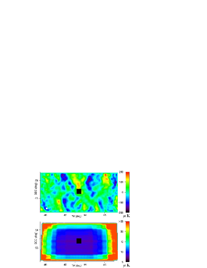
Figure 1: The top panel shows the LMT-differenced, atmospheric mode removed, noise weighted, coadded map for the CMB5 field. The guide quasar has been replaced with black pixels. The small white circle in the lower left hand corner of the map represents the FWHM of the average array element beam size as determined from the coadded quasar image. The map is pixelated at $2.5^{\prime}$ and has been smoothed with a $4.5^{\prime}$ FWHM Gaussian. The predominance of extended structure in the vertical direction results from de-projection of extended horizontal structure during atmospheric mode removal. The lower panel shows the noise in the LMT differenced map as a function of position. The S/N the degree-scale structures in this map approach 100. This figure is from Kuo et al. (2002).

The maximum likelihood band powers are estimated iteratively using the quadratic iteration method (Bond et al. 1998). The Acbar power spectrum – as well as the power spectra from other contemporary experiments – is shown in Figure 2. The decorrelated band powers and window functions are available on the Acbar website.

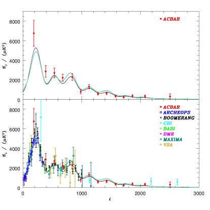
Figure 2: Top Panel: The Acbar CMB power spectrum, ${\mathcal{C}}_{\ell}\equiv\ell(\ell+1)C_{\ell}/{(2\pi)}$, plotted over a vacuum energy dominated [$\Omega_{k}=-0.05$, $\Omega_{\Lambda}=0.5$, $\omega_{cdm}=0.12$, $\omega_{b}=0.02$, $H_{0}=50$, $\tau_{C}=0.025$, $n_{s}=0.925$, amplitude ${\mathcal{C}}_{10}=1.11\times 10^{-10}T_{\rm CMB}^{2}$] model (black thin line) and a CDM dominated [$\Omega_{k}=0.05$, $\Omega_{\Lambda}=0$, $\omega_{cdm}=0.22$, $\omega_{b}=0.02$, $H_{0}=50$, $\tau_{C}=0$, $n_{s}=0.925$, amplitude ${\mathcal{C}}_{10}=1.34\times 10^{-10}T_{\rm CMB}^{2}$] model (green thick line). These are the best-fit models, for $\Lambda$ and $\Lambda$-free models respectively, found during the Acbar+Others parameter estimation described Goldstein et al. (2002), with the weak-$h$ prior. Bottom Panel: The top panel with the addition of power spectra from several other experiments. Both models appear to be reasonable fits to the data, with the $\Omega_{\Lambda}=0.5$ model statistically being the better of the two. This figure is from Goldstein et al. (2002).

5 Systematic Tests

We performed a number of systematic checks upon the Acbar data to verify the robustness of the measured power spectrum. Of particular concern was the effect of possible foreground contamination. We selected the target regions on the sky to have low dust contrast from the IRAS/DIRBE maps of Finkbeiner et al. (1999) extrapolated to 150 GHz. We estimate the total variance in the LMT-differenced maps due to dust at 150 GHz to be about 9 $\mu$K² and 70 $\mu$K² for CMB2 and CMB5, respectively. In addition, unresolved point sources may also contribute power to the maps. We project out the central pointing sources in each field and a bright radio galaxy (Pictor A) in the CMB2 field. We detect only one other PMN radio source at greater than $3\sigma$ and it too is removed. We investigated the potential effects of these foregrounds by generating the power spectrum with no additional foreground removal and then re-calculating it after projecting out the IRAS/DIRBE template and all 170 PMN sources in the CMB fields above 40 mJy at 5 GHz. The foreground removal has a negligible impact on the power spectrum indicating an insignificant level of contamination. We use the foreground-removed power spectrum for all subsequent analysis.

We also performed a number of “jackknife” tests on the data. We divided each CMB data set into a first-half and second-half and calculated the power spectra to look for systematic changes over time. We also broke the data into left-going and right-going chopper sweeps to look for direction-dependent effects. Finally, we divided the data into $180^{\circ}$ azimuth chunks either towards or away from the near-by Martin A. Pomerantz Observatory (MAPO) building to investigate pick-up from sources at low elevation. The power spectrum passed all three jackknife tests within the error bars (determined by Monte Carlo simulation).

6 Cosmological Parameter Extraction

6.1 Method

In this section we describe using the CMB power spectrum measured by Acbar and other CMB experiments to derive Bayesian estimates of cosmological parameters in inflation-motivated adiabatic CDM models. A more complete treatment is presented in Goldstein et al. (2002). Our set of cosmological parameters includes $\Omega_{k}=(1-\Omega_{tot})$, $\Omega_{\Lambda}$, $\omega_{cdm}$, $\omega_{b}$, $n_{s}$, $\tau_{C}$, $\ln{{\mathcal{C}}_{10}}$. The total energy density ($\Omega_{tot}$) is the sum of the energy density from the vacuum ($\Omega_{\Lambda}$), matter, and relativistic particles. The matter density is split into two constituents: baryonic matter ($\Omega_{b}\equiv\omega_{b}/h^{2}$) and cold dark matter ($\Omega_{cdm}\equiv\omega_{cdm}/h^{2}$), where $h$ is the Hubble parameter in units of 100 km/s/Mpc. $n_{s}$ is the scalar index of primordial perturbations. The amplitude of the power spectrum at $\ell=10$ ($\ln{{\mathcal{C}}_{10}}$) gives the overall amplitude of the primordial fluctuations and has been well constrained by the COBE-DMR (Bennett et al. 1996) [used in the parameter analysis in Goldstein et al. (2002)] and more recently by WMAP (Hinshaw et al. 2003).

The universe reionized at some point between decoupling and the present. After reionization, CMB photons scatter further. $\tau_{C}$ is the Compton optical depth (from decoupling to present) due to such scattering. High $\tau_{C}$ diminishes CMB power by a factor of $\exp[-2\tau_{C}]$ over most of the $\ell$ range in the $TT$ spectrum, though not in the DMR range. After the parameter estimates in Goldstein et al. (2002) were derived, the WMAP team reported a significant detection of the reionization signature with a best-fit $\tau_{C}=0.17\pm 0.04$ from an excess in the $TE$ cross-spectrum at low-$\ell$ (Kogut et al. 2003). The Acbar results have assumed no prior on $\tau_{C}$ but re-analysis in the light of the WMAP results is underway.

Because of the high resolution of Acbar, it is possible that sources of secondary anisotropy, such as from the Sunyaev-Zel’dovich effect in clusters, could contribute significant power above the primary CMB spectrum at high-$\ell$. However, the detection of power in the highest $\ell$ bin is only $0.9\sigma$ above the best-fit model CMB power spectrum. Thus, for cosmological parameter estimation based on the full Acbar power spectrum we believe we can safely ignore the effects from the potential SZ contamination. As the precision of our high-$\ell$ data improves, however, we will have to include the SZ contribution in deriving parameter estimates.

We also derive four observable quantities from the seven basic parameters. These are the present age of the Universe ($t_{0}$), the Hubble parameter ($h$), the variance in the linear density fluctuation spectrum smoothed on $8h^{-1}$ Mpc scales ($\sigma_{8}^{2}$), and the effective shape parameter of the linear density power spectrum ($\Gamma_{eff}$). The values of the derived parameters are calculated at each point on the parameter grid but do not reflect additional information; they are used for incorporating prior constraints from other data sets, such as the value of the Hubble parameter from HST or the value of $\sigma_{8}\Omega_{m}^{0.56}$ from large scale structure (LSS) surveys. The individual priors are described in detail in Goldstein et al. (2002).

6.2 Results

By applying the method described above we can investigate the power of adding Acbar to the various data sets. We can also investigate the effects of applying different priors upon the results. As a first test we computed the 1D parameter likelihoods by adding Acbar to the COBE-DMR power spectrum (Bond et al. 1998). The thought is that the COBE data provides a low-$\ell$ anchor to the power spectrum and the precise high-$\ell$ measurements of Acbar will be sensitive to the physics of the damping tail. In particular, the strength of the viscous and diffusive couplings are sensitive to baryon density, $\omega_{b}$ (White 2001).

However, what we found is that the degenerate influence of other cosmological parameters upon the damping tail (e.g., $\Omega_{M}$ and $n_{s}$) prevents a precise measurement of $\omega_{b}$ without prior knowledge from the peak-dip structure at lower-$\ell$ (degenerates are always causing problems such as this). In addition, some of the parameter results are found to depend upon assumed priors. Once we include information on the power spectrum from experiments at lower $\ell$ the Acbar data improves constraints on parameters by virtue of the small error bars. The best-fit parameters of the joint data set are found to be stable to the application of priors and are reproduced in Table 1.

Table 1: Parameter Estimates and Errors

Priors	Run	$\Omega_{tot}$	$n_{s}$	$\Omega_{b}h^{2}$	$\Omega_{cdm}h^{2}$	$\Omega_{\Lambda}$	$\Omega_{m}$	$\Omega_{b}$	$h$	Age	$\tau_{C}$
weak–$h$
	Others	$1.03^{0.05}_{0.04}$	$0.96^{0.09}_{0.05}$	$0.022^{0.003}_{0.002}$	$0.13^{0.03}_{0.03}$	$0.53^{0.18}_{0.19}$	$0.50^{0.19}_{0.19}$	$0.072^{0.023}_{0.023}$	$0.57^{0.11}_{0.11}$	$14.9^{1.3}_{1.3}$	$<0.48$
	Acbar +Others	$1.04^{0.04}_{0.04}$	$0.95^{0.09}_{0.05}$	$0.022^{0.003}_{0.002}$	$0.12^{0.03}_{0.03}$	$0.57^{0.16}_{0.18}$	$0.47^{0.18}_{0.18}$	$0.071^{0.022}_{0.022}$	$0.57^{0.11}_{0.11}$	$15.1^{1.3}_{1.3}$	$<0.47$
HST–$h$
	Others	$1.00^{0.03}_{0.03}$	$0.99^{0.07}_{0.07}$	$0.022^{0.003}_{0.003}$	$0.12^{0.03}_{0.02}$	$0.68^{0.09}_{0.12}$	$0.33^{0.11}_{0.11}$	$0.049^{0.013}_{0.013}$	$0.68^{0.08}_{0.08}$	$13.7^{1.0}_{1.0}$	$<0.45$
	Acbar +Others	$1.00^{0.03}_{0.02}$	$0.97^{0.07}_{0.06}$	$0.022^{0.003}_{0.002}$	$0.12^{0.02}_{0.02}$	$0.70^{0.07}_{0.10}$	$0.31^{0.10}_{0.10}$	$0.049^{0.013}_{0.013}$	$0.68^{0.08}_{0.08}$	$13.9^{0.9}_{0.9}$	$<0.43$
wk–$h$+flat
	Others	(1.00)	$0.95^{0.08}_{0.05}$	$0.022^{0.003}_{0.002}$	$0.13^{0.03}_{0.03}$	$0.59^{0.15}_{0.23}$	$0.43^{0.19}_{0.19}$	$0.056^{0.014}_{0.014}$	$0.63^{0.10}_{0.10}$	$13.9^{0.5}_{0.5}$	$<0.34$
	Acbar +Others	(1.00)	$0.95^{0.07}_{0.05}$	$0.022^{0.002}_{0.002}$	$0.13^{0.02}_{0.02}$	$0.66^{0.10}_{0.16}$	$0.35^{0.15}_{0.15}$	$0.049^{0.011}_{0.011}$	$0.67^{0.09}_{0.09}$	$13.8^{0.4}_{0.4}$	$<0.31$
	Acbar +Others
wk–$h$+LSS		$1.03^{0.05}_{0.04}$	$0.98^{0.09}_{0.07}$	$0.022^{0.003}_{0.003}$	$0.11^{0.02}_{0.03}$	$0.64^{0.08}_{0.12}$	$0.41^{0.11}_{0.11}$	$0.067^{0.019}_{0.019}$	$0.59^{0.09}_{0.09}$	$15.2^{1.4}_{1.4}$	$<0.51$
wk–$h$+flat+LSS		(1.00)	$0.94^{0.07}_{0.05}$	$0.022^{0.002}_{0.002}$	$0.13^{0.02}_{0.02}$	$0.65^{0.08}_{0.11}$	$0.36^{0.10}_{0.10}$	$0.050^{0.008}_{0.008}$	$0.66^{0.07}_{0.07}$	$13.9^{0.4}_{0.4}$	$<0.32$
wk–$h$+flat+LSS($low$–$\sigma_{8}$)		(1.00)	$0.98^{0.07}_{0.06}$	$0.022^{0.002}_{0.002}$	$0.12^{0.02}_{0.02}$	$0.71^{0.06}_{0.07}$	$0.28^{0.07}_{0.07}$	$0.044^{0.006}_{0.006}$	$0.71^{0.07}_{0.07}$	$13.7^{0.4}_{0.4}$	$<0.34$
strong data		$1.01^{0.03}_{0.02}$	$0.99^{0.07}_{0.05}$	$0.023^{0.003}_{0.002}$	$0.12^{0.02}_{0.02}$	$0.70^{0.05}_{0.05}$	$0.31^{0.05}_{0.05}$	$0.051^{0.011}_{0.011}$	$0.67^{0.05}_{0.05}$	$14.1^{0.9}_{0.9}$	$<0.49$
strong data+flat		(1.00)	$0.97^{0.05}_{0.05}$	$0.022^{0.002}_{0.002}$	$0.12^{0.01}_{0.01}$	$0.70^{0.04}_{0.05}$	$0.30^{0.04}_{0.04}$	$0.046^{0.004}_{0.004}$	$0.69^{0.04}_{0.04}$	$13.7^{0.2}_{0.2}$	$<0.32$
strong data+flat+LSS($low$–$\sigma_{8}$)		(1.00)	$0.97^{0.05}_{0.05}$	$0.022^{0.002}_{0.002}$	$0.12^{0.01}_{0.01}$	$0.71^{0.05}_{0.04}$	$0.28^{0.05}_{0.05}$	$0.045^{0.004}_{0.004}$	$0.70^{0.04}_{0.04}$	$13.7^{0.2}_{0.2}$	$<0.31$

Note. — Parameter estimates and errors for several prior combinations with and without Acbar. Errors are quoted at 1–$\sigma$ (16% and 84% points of the integral of the likelihood), except for $\tau_{C}$ where the 95% upper-limit is given. The various priors are described in Goldstein et al. (2002). The top block lists results found with and without the inclusion of Acbar data, which shows the small improvements found upon adding Acbar to the mix. The bottom block shows the effect of applying stronger priors on the Acbar+Others dataset, which naturally leads to improvements on the parameter estimates. The difference between the LSS and LSS(low-$\sigma_{8}$) priors does lead to several slight shifts, smaller than the 1–$\sigma$ errors. This table is reproduced from Goldstein et al. (2002).

One would expect that the addition of high sensitivity data at high-$\ell$ would lead to significant improvements upon the parameter that controls the scale of damping ($\omega_{b}$) and the tilt ($n_{s}$) because of the increased $\ell$ baseline; but that appears not to be the case, as evidenced in Table 1. It is likely that the near degeneracies between certain parameter pairs [see, for example, Efstathiou & Bond (1999)] implies that improved precision of measurement does not necessarily translate into significant improvements in the 1D parameter likelihoods. However, we can measure the power of a data set to constrain cosmological parameter space by determining the set of parameter “eigenmodes” that are most well constrained by the likelihood. We calculated the parameter eigenmodes and associated eigenvalue uncertainty for the set of CMB data before Acbar and then re-calculated the eigenvectors including the Acbar data.

Most of the eigenvectors are dominated by one or two parameters and it is interesting to note that the eigenvector most improved by inclusion of the Acbar data is dominated by $\Omega_{\Lambda}$. The eigenvectors are orthogonal and thus the product of their uncertainties represents a “volume” of parameter space consistent with the data. We find that including the Acbar data set reduces the volume of acceptable $\Lambda$CDM parameter space by a factor of $\sim 3$. This shows that roughly $2/3$ of the previously consistent parameter space has been eliminated by inclusion of the Acbar data, but this is not reflected in the marginalized likelihoods of the fiducial parameters.

As mentioned above, the addition of the Acbar data has a substantial impact on the likelihood of models without a cosmological constant. The $3\sigma$ lower-limit is increased from $\Omega_{\Lambda}>0.086$ for the “Other” CMB experiments to $\Omega_{\Lambda}>0.136$ by including Acbar. The $\chi^{2}$ of best-fit free-$\Omega_{\Lambda}$ and $\Omega_{\Lambda}=0$ models is $\chi^{2}=140$ and $\chi^{2}=160$ for 116 band powers, respectively. The probably that the dark energy density is zero has become significantly unlikely.

In addition to estimating cosmological parameters from the primary power spectrum, we also derived constraints on $\sigma_{8}$ from secondary anisotropy resulting from a background of unresolved SZ clusters (Komatsu & Seljak 2002). We employed two model SZ power spectra: one generated from Smoothed Particle Hydrodynamics (SPH) simulations (Bond et al. 2002) and the other an analytical model (Zhang et al. 2002). The amplitude of the SZ power spectrum is expected to depend very strongly upon the value of $\sigma_{8}$ going roughly as ${\mathcal{C}}_{\ell}^{SZ}\sim(\Omega_{b}h)^{2}\sigma_{8}^{7}$. This strong dependence should allow significant constraints to be placed upon $\sigma_{8}$ with existing (and to a higher degree with forthcoming) high-$\ell$ data sets from Acbar, CBI (Mason et al. 2002), and BIMA (Dawson et al. 2002).

For this analysis we only use power spectrum data points above $\ell\gtrsim{1500}$. Although the primary power spectrum is falling rapidly for $\ell{>}2000$, its contribution compared to the SZ signal is by no means negligible; particularly at 150 GHz. We include the contribution from the best-fit power spectrum of the “Acbar+Others” data set in our analysis ($\Omega_{b}=0.047$, $\Omega_{cdm}=0.253$, $\Omega_{\Lambda}=0.7$, $h=0.69$, $n_{s}=0.975$, and $\tau_{C}=0.2$). We account for the difference between our best-fit cosmology and the one used to generate the SZ power spectra ($\Omega_{b}h=0.035$) by using $\sigma_{8}^{SZ}=(\Omega_{b}h/0.035)^{0.29}\sigma_{8}$. We also include the effects of the non-Gaussian nature of the SZ signal upon the sample variance [see Goldstein et al. (2002) for a discussion].

We find a best-fit value of $\sigma_{8}^{SZ}=0.98^{+0.12}_{-0.21}$ for the joint Acbar, CBI, and BIMA data set using the analytical model and a slightly higher value of 1.04 for the SPH model. These values of $\sigma_{8}$ are on the high-end of values determined from LSS measurements. It is possible that the excess power on small scales measured by CMB experiments may be the result of high-redshift supernova from the first stars (Oh et al. 2003). On the other hand, it may simply reflect a current lack of understanding of the SZ power spectrum. The best-fit values of $\sigma_{8}^{SZ}$ measured by Acbar at 150 GHz are consist with those measured by CBI and BIMA at 30 GHz within $1\sigma$. Although the Acbar data alone do not yield a $3\sigma$ lower limit to $\sigma_{8}$, the combination of Acbar, CBI, and BIMA data results in a $3\sigma$ lower limit of $\sigma_{8}^{SZ}>0.63$ (including non-Gaussian effects) within the context of the SZ models tested.

7 Discussion

The Acbar experiment has been used to precisely measure the CMB sky from the South Pole and has produced the highest signal-to-noise map of the CMB to date. This data has yielded the most sensitive measurement of the damping tail region of the CMB power spectrum as of this writing; analysis of the remainder of the 2001 through 2002 Acbar data is underway and should further refine our power spectrum and parameter estimates. The data agree with the predictions of the flat-$\Lambda$CDM model with adiabatic initial perturbations. When considering the Acbar data in combination with other contemporary CMB results, the addition of a single parameter, $\Omega_{\Lambda}$, significantly improves the fit to the data with a $\Delta\chi^{2}=20$.

We find that the addition of the high sensitivity Acbar data the the current CMB data does not lead to significant reductions of the $1\sigma$ uncertainties in the canonical cosmological parameters. However, when considered in the eigenmode basis of the parameter likelihood space, the addition of the Acbar data results in a significant reduction of the observationally acceptable parameter space; this indicates that the lack of improved errors on the fundamental parameters probably results from degeneracies between the fiducial parameters. The very high-$\ell$ points of the Acbar power spectrum indicate a slight excess of power at 150 GHz that is consistent with a value of $\sigma_{8}$ on the upper-end of limits from LSS if the excess is due to SZ emission from clusters and is consistent with CBI and BIMA at 30 GHz. However, the Acbar data alone do not place to a $2\sigma$ lower-limit on the detection of this excess power.

It is clear from the measured CMB power spectrum in Figure 2 that the Acbar and CBI data are consistent with each other as well as the underlying $\Lambda$CDM cosmological model. This is significant for a number of reasons. First, these experiments have pushed the $\ell$-space coverage of the CMB power spectrum to a factor of $\sim{3}$ larger than previous experiments. The remarkable agreement of the data with the predictions of a $\Lambda$CDM cosmology across such a large range of angular scale adds substantial credibility to the underlying model by testing the physics of the damping region which are complementary to the accoustic peaks. The high-$\ell$ data have provided an essential test that the $\Lambda$CDM model has passed with flying colors. Second, the Acbar and CBI data were taken by completely different experimental techniques (quasi-total power bolometers versus interferometric measurements) at significantly different observing frequencies (150 GHz for Acbar versus 30 GHz for CBI). The sensitivity of the two experiments to systematic effects are quite different and the consistency of the data sets is reasuring.

After publication of the Acbar results in late 2002, the WMAP team released their phenomenal first-year power spectrum and cosmological parameters (Hinshaw et al. 2003; Spergel et al. 2003). This power spectrum runs out of steam in the vicinity of the third doppler peak ($\ell\sim 800$) and the Acbar and CBI data sets were used to “extend” the WMAP power spectrum (forming the WMAPext data set). The damping tail data helps break some of the degeneracies at low-$\ell$ and also provides marginal evidence for a “running” scalar index, $dn_{s}/d\ln{k}\neq 0$ (Spergel et al. 2003) that is bolstered by incorporation of galaxy redshift and Lyman-$\alpha$ survey results. The value of the scalar index and running can be used to constrain inflationary models; already CMB data have been used to rule out inflationary potentials of the form $V(\phi)\propto\phi^{4}$ at $3\sigma$ (Kinney et al. 2003). More precise data in the damping tail region should assist in this endeavor.

The Acbar program has been primarily supported by NSF office of polar programs grants OPP-8920223 and OPP-0091840. This research used resources of the National Energy Research Scientific Computing Center, which is supported by the Office of Science of the U.S. Department of Energy under Contract No. DE-AC03-76SF00098. Chao-Lin Kuo acknowledges support from a Dr. and Mrs. CY Soong fellowship and Marcus Runyan acknowledges support from a NASA Graduate Student Researchers Program fellowship. Chris Cantalupo, Matthew Newcomb and Jeff Peterson acknowledge partial financial support from NASA LTSA grant NAG5-7926.

References

- Bennett et al. (1996) Bennett, C. L., Banday, A. J., Gorski, K. M., Hinshaw, G., Jackson, P., Keegstra, P., Kogut, A., Smoot, G. F., Wilkinson, D. T., & Wright, E. L. 1996, ApJ, 464, L1
- Bond et al. (1998) Bond, J. R., Jaffe, A. H., & Knox, L. 1998, Phys. Rev. D, 57, 2117
- Bond et al. (2002) Bond, J. R., Ruetalo, M. I., Wadsley, J. W., & Gladders, M. D. 2002, in ASP Conf. Ser. 257: AMiBA 2001: High-Z Clusters, Missing Baryons, and CMB Polarization, 15–+
- Dawson et al. (2002) Dawson, K. S., Holzapfel, W. L., Carlstrom, J. E., Joy, M., LaRoque, S. J., & Reese, E. D. 2002, ApJ, in press, astro-ph/020601
- Efstathiou & Bond (1999) Efstathiou, G. & Bond, J. R. 1999, MNRAS, 304, 75
- Finkbeiner et al. (1999) Finkbeiner, D. P., Davis, M., & Schlegel, D. J. 1999, ApJ, 524, 867
- Goldstein et al. (2002) Goldstein, J., Ade, A. R., Bock, J. J., Bond, J. R., Cantalupo, C., Cantaldi, C., Daub, M. D., Holzapfel, W. L., Kuo, C. L., Lange, A. E., Lueker, M., Newcomb, M., Peterson, J. B., Pogosyan, D., Ruhl, J., Runyan, M. C., & Torbet, E. 2002, ApJ submitted, astro-ph/0212517
- Hinshaw et al. (2003) Hinshaw, G., Spergel, D. N., Verde, L., Hill, R. S., Meyer, S. S., Barnes, C., Bennett, C. L., Halpern, M., Jarosik, N., Kogut, A., Komatsu, E., Limon, M., Page, L., Tucker, G. S., Weiland, J., Wollack, E., & Wright, E. L. 2003, Submitted to ApJ, preprint: astro
- Kinney et al. (2003) Kinney, W. H., Kolb, E. W., Melchiorri, A., & Riotto, A. 2003, FERMILAB-Pub-03/117-A, preprint: hep-ph/0305130
- Kogut et al. (2003) Kogut, A., Spergel, D. N., Barnes, C., Bennett, C. L., Halpern, M., Hinshaw, G., Jarosik, N., Limon, M., Meyer, S. S., Page, L., Tucker, G., Wollack, E., & Wright, E. L. 2003, Submitted to ApJ, astro
- Komatsu & Seljak (2002) Komatsu, E. & Seljak, U. 2002, MNRAS, 336, 1256
- Kuo et al. (2002) Kuo, C. L., Ade, P. A. R., Bock, J. J., Cantalupo, C., Daub, M. D., Goldstein, J. H., Holzapfel, W. L., Lange, A. E., Lueker, M., Newcomb, M., Peterson, J. B., Ruhl, J., Runyan, M. C., & Torbet, E. 2002, ApJ submitted, astro-ph/0212289
- Lay & Halverson (2000) Lay, O. P. & Halverson, N. W. 2000, ApJ, 543, 787
- Lee et al. (2001) Lee, A. T., Ade, P., Balbi, A., Bock, J., Borrill, J., Boscaleri, A., de Bernardis, P., Ferreira, P. G., Hanany, S., Hristov, V. V., Jaffe, A. H., Mauskopf, P. D., Netterfield, C. B., Pascale, E., Rabii, B., Richards, P. L., Smoot, G. F., Stompor, R., Winant, C. D., & Wu, J. H. P. 2001, ApJ, 561, L1
- Mason et al. (2002) Mason, B. S., Pearson, T., Readhead, A. C. S., Shephard, M. C., Sievers, J. L., Udomprasert, P. S., Cartwright, J. K., Farmer, A. J., Padin, S., Myers, S. T., Bond, J. R., Contaldi, C. R., Pen, U.-L., Prunet, S., Pogosyan, D., Carlstom, J. E., Kovac, J., Leitch, E., Pryke, C., Halverson, N., Holzapfel, W., Altamirano, P., Brofman, L., Casassus, S., May, J., & Joy, M. 2002, Submitted to ApJ, astro-ph/0205384
- Netterfield et al. (2002) Netterfield, C. B., Ade, P. A. R., Bock, J. J., Bond, J. R., Borrill, J., Boscaleri, A., Coble, K., Contaldi, C. R., Crill, B. P., de Bernardis, P., Farese, P., Ganga, K., Giacometti, M., Hivon, E., Hristov, V. V., Iacoangeli, A., Jaffe, A. H., Jones, W. C., Lange, A. E., Martinis, L., Masi, S., Mason, P., Mauskopf, P. D., Melchiorri, A., Montroy, T., Pascale, E., Piacentini, F., Pogosyan, D., Pongetti, F., Prunet, S., Romeo, G., Ruhl, J. E., & Scaramuzzi, F. 2002, ApJ, 571, 604
- Oh et al. (2003) Oh, S. P., Cooray, A., & Kamionkowski, M. 2003, preprint: astro-ph/0303007
- Peterson et al. (2002) Peterson, J. B., Radford, S. J. E., Ade, P. A. R., Chamberlin, R. A., O’Kelly, M. J., Peterson, K. M., & Schartman, E. 2002, PASP submitted, astro-ph/0211134
- Romer et al. (2003) Romer, A. K., Gomez, P. L., & Collaboration, T. A. 2003, in Carnegie Observatories Astrophysics Series, Vol. 3: Clusters of Galaxies: Probes of Cosmological Structure and Galaxy Evolution, ed. J. S. Mulchaey, A. Dressler, & A. Oemler (Pasadena: Carnegie Observatories), http://www.ociw.edu/ociw/symposia/series/symposium3/proceedings.html
- Runyan et al. (2003a) Runyan, M. C., Ade, P. A. R., Bhatia, R. S., Bock, J. J., Daub, M. D., Goldstein, J. H., Haynes, C. V., Holzapfel, W. L., Kuo, C. L., Lange, A. E., Leong, J., Lueker, M., Newcomb, M., Peterson, J. B., Ruhl, J., Sirbi, G. I., Torbet, E., Tucker, C., Turner, A. D., & Woolsey, D. 2003a, ApJ submitted, astro-ph/0303515
- Runyan et al. (2003b) Runyan, M. C., Ade, P. A. R., Bock, J. J., Cantalupo, C., Daub, M. D., Goldstein, J. H., Gomez, P., Holzapfel, W. L., Kuo, C. L., Lange, A. E., Lueker, M., Newcomb, M., Peterson, J. B., Romer, A. K., Ruhl, J., & Torbet, E. 2003b, In Preparation
- Spergel et al. (2003) Spergel, D. N., Verde, L., Peiris, H. V., Komatsu, E., Nolta, M. R., Bennett, C. L., Halpern, M., Hinshaw, G., Jarosik, N., Kogut, A., Limon, M., Meyer, S. S., Page, L., Tucker, G. S., Weiland, J. L., Wollack, E., & Wright, E. L. 2003, Submitted to ApJ, Preprint: astro
- Turner et al. (2001) Turner, A. D., Bock, J. J., Beeman, J. W., Glenn, J., Hargrave, P. C., Hristov, V. V., Nguyen, H. T., Rahman, F., Sethuraman, S., & Woodcraft, A. L. 2001, Appl. Opt., 40, 4921
- White (2001) White, M. 2001, ApJ, 555, 88
- Zhang et al. (2002) Zhang, P., Pen, U., & Wang, B. 2002, ApJ, 577, 555