Gauss–Legendre Sky Pixelization (GLESP) for CMB maps

A new scheme of sky pixelization is developed for CMB maps. The scheme is based on the Gauss–Legendre polynomials zeros and allows one to create strict orthogonal expansion of the map. A corresponding code has been implemented and comparison with other methods has been done.

1 Introduction

Starting from the COBE experiment using the so called Quadrilateralized Sky Cube Projection (see Chan and O’Neill¹ 1976, O’Neill and Laubscher² 1976, Greisen and Calabretta³ 1993), the problem of the whole sky CMB pixelization has attracted great interest. At least three methods of the CMB celestial sphere pixelization have been proposed and implemented after the COBE pixelization scheme: the Icosahedron pixelizing by Tegmark⁴ (1996), the Igloo pixelization by Crittenden and Turok⁵ (1998, hereafter CT98) and the HEALPix method by Górski et al.⁶ (1999) (with the last modification in 2003). Two important questions mentioned already by Tegmark⁴ (1996) are now under discussion: a) what is the optimal method for the choice of the $N_{pix}$ positions of pixel centers, shapes and sizes to provide (as good as possible) the compact uniform coverage of the sky by pixels with equal areas, and b) what is the best way to approximate any convolutions of the maps by sums using pixels ?

All the above mentioned pixelization schemes were devoted to solve the first problem as accurate as possible, and the answer to the second question usually follows for the chosen pixelization scheme.

In this paper we change the focus of the problem to processing on the sphere and then determine the scheme of pixelization. We would like to remind that pixelization of the CMB data on the sphere is only some part of the general problem, which is the determination of the coefficients of the spherical harmonic decomposition of the CMB signal for both anisotropy and polarization. These coefficients, which we call $a_{\ell m}$, are used in subsequent steps in the analysis of the measured signal, and in particular, in the determination of the power spectra, $C_{\ell}$, of the anisotropy and polarization (see review in Hivon at al,⁷ 2002), in some special methods for components separation (Stolyarov et al.⁸ 2002; Naselsky et al.⁹ 2003a) and phase statistics (Chiang et al.¹⁰ 2003; Naselsky et al.^11,12 2003b, 2004; Coles et al.¹³ 2004).

Here we propose a specific method to calculate the coefficients $a_{\ell m}$. It is based on the so called Gaussian quadratures and is presented in Sec. 2 . In this specific pixelization scheme correspond the position of pixel centers along the $\theta$–coordinate to so–called the Gauss–Legendre quadrature zeros and it will be shown (Sec. 5) that this method increases the accuracy of calculations essentially.

Thus, the method of calculation of the coefficients $a_{\ell m}$ dictates the method of the pixelization. We call our method GLESP, the Gauss–Legendre Sky Pixelization. We have developed a special code for the GLESP approach and a package of codes which are necessary for the whole investigation of the CMB data including the determination of anisotropy and polarization power spectra, $C_{\ell}$, the Minkowski functionals and other statistics.

This paper is devoted to description of the main idea of the GLESP method, the estimation of the accuracy of the different steps and of the final results, the description of the GLESP code and its testing. We do not discuss the problem of integration over a finite pixel size for the time ordered data in this paper. The simplest scheme of integration over pixel area is to use equivalent weight relatively to the center of the pixel. The GLESP code uses this method as HEALPix and Igloo do.

In forthcoming papers we shall discuss our GLESP code extension on the processing of CMB polarization data, the Minkowski functionals and the peak statistics of CMB maps.

2 Main ideas and basic relations

The standard decomposition of the measured temperature variations on the sky, $\Delta T(\theta,\phi)$, in spherical harmonics is

$$\Delta T(\theta,\phi)=\sum_{\ell=2}^{\infty}\sum_{m=-\ell}^{m=\ell}a_{\ell m}Y_{\ell m}(\theta,\phi)\$$ (1)

$$Y_{\ell m}(\theta,\phi)=\sqrt{{(2\ell+1)\over 4\pi}{(\ell-m)!\over(\ell+m)!}}P_{\ell}^{m}(x)e^{im\phi},\leavevmode\nobreak\ x=\cos\theta\,,$$ (2)

where $P_{\ell}^{m}(x)$ are the associated Legendre polynomials. For a continuous $\Delta T(x,\phi)$ function, the coefficients of decomposition, $a_{\ell m}$, are

$$a_{\ell m}=\int^{1}_{-1}dx\int^{2\pi}_{0}d\phi\Delta T(x,\phi)Y^{*}_{\ell m}(x,\phi)$$ (3)

where $Y^{*}_{\ell m}$ denotes complex conjugation of $Y_{\ell m}$. For numerical evaluation of the integral Eq(3) we will use the Gaussian quadratures, a method which was proposed by Gauss in 1814, and developed later by Christoffel in 1877. As the integral over $x$ in Eq(3) is an integral over a polynomial of $x$ we may use the following equality (Press et al.¹⁴ 1992)

$$\int^{1}_{-1}dx\Delta T(x,\phi)Y^{*}_{\ell m}(x,\phi)=\sum^{N}_{j=1}w_{j}\Delta T(x_{j},\phi)Y^{*}_{\ell m}(x_{j},\phi)\,.$$ (4)

where $w_{j}$ is a proper Gaussian quadrature weighting function. Here the weighting function $w_{j}=w(x_{j})$ and $\Delta T(x_{j},\phi)Y^{*}_{\ell m}(x_{j},\phi)$ are taken at points $x_{j}$ which are the net of roots of the Legendre polynomial

$$P_{N}(x_{j})=0\,,$$ (5)

where $N$ is the maximal rank of the polynomial under consideration. It is well known that the equation $P_{N}(x_{j})=0$ has $N$ number of zeros in interval $-1\leq x\leq 1$. For the Gaussian–Legendre method Eq(4), the weighting coefficients are (Press et al.¹⁴ 1992)

$$w_{j}={2\over 1-x^{2}_{j}}[P_{N}^{{}^{\prime}}(x_{j})]^{-2}\,,$$ (6)

where ^′ denotes a derivative. They can be calculated together with the set of $x_{j}$ with the ‘gauleg’ code (Press et al.¹⁴ 1992, Sec. 4.5).

Figure 1: Gauss-Legendre weighting coefficients ($w_{j}$) versus Legendre polynomial zeros ($x_{j}=\cos\theta_{j}$) being centers of rings used in GLESP for the case of $N=31$. Positions of zeros are plotted by vertical lines.

Figure 2: Ring center position ($x_{j}=\cos\theta_{j}$) vs ring number for 2 pixelization schemes, HEALPix (solid) and GLESP (dashed). Figure demonstrates the case of $N=31$.

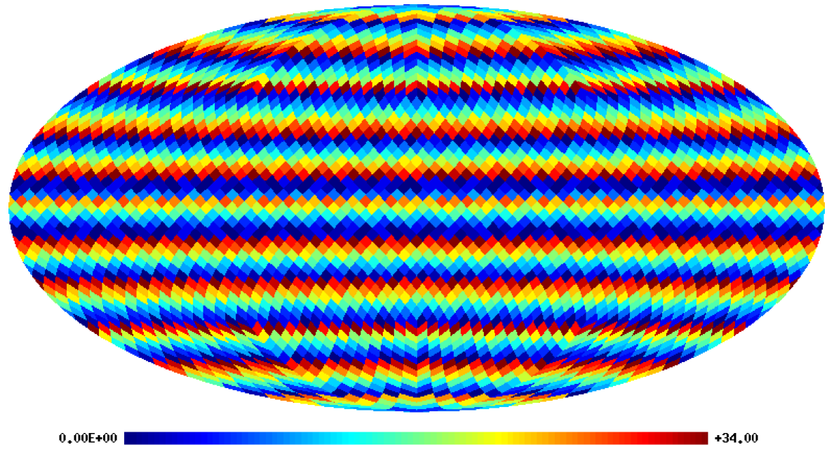
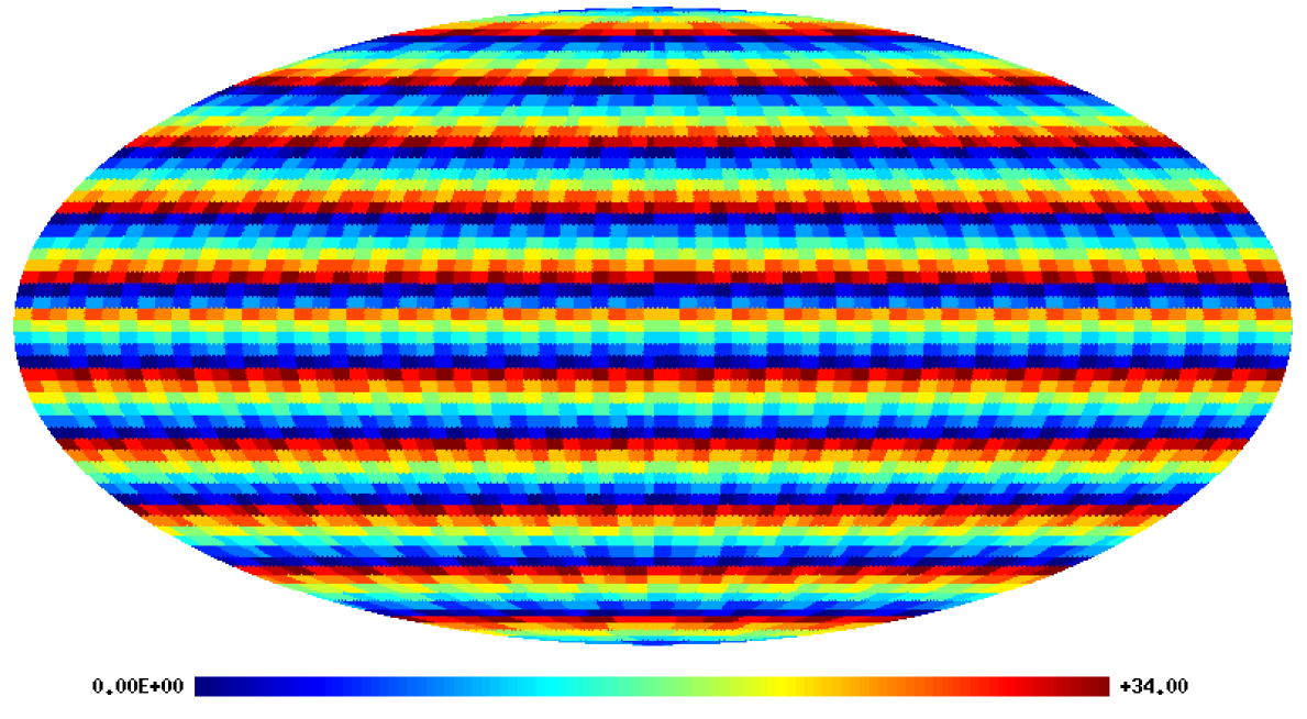
Figure 3: Schematic representation of 2 types of pixelization on sphere: HEALPix (top) and GLESP (bottom). Various color of pixels is used to show their shape.

In the GLESP approach are the trapezoidal pixels bordered by $\theta$ and $\phi$ coordinate lines with the pixel centers (in the $\theta$ direction) situated at points with $x_{j}=\cos\theta_{j}$. Thus, the interval $-1\leq x\leq 1$ is covered by $N$ rings of the pixels (details are given in Sec. 3). The angular resolution achieved in the measurement of the CMB data determines the upper limit of summation in Eq. (1), $\ell\leq\ell_{max}$. To avoid the Nyquist restrictions we use a number of pixel rings, $N\geq 2\ell_{max}$. In order to make the pixels in the equatorial ring (along the $\phi$ coordinate) nearly squared, the number of pixels in this direction should be $N_{\phi}^{max}\approx 2N$. The number of pixels in other rings, $N_{\phi}^{j}$, must be determined from the condition of making the pixel sizes as equal as possible with the equatorial ring of pixels.

Fig. 1 shows the weighting coefficients, $w_{j}$, and the position of pixel centers for the case $N=31$. Fig. 2 compares some features of the pixelization schemes used in HEALPix and GLESP (see Sec. 4). Fig. 3 compares pixel distribution and shapes on a sphere in the mollview projections of HEALPix and in GLESP.

In the definition (1) are the coefficients $a_{\ell m}$ complex quantities while $\Delta T$ is real. In the GLESP code started from the definition (1) we use the following representation of the $\Delta T$

$$\Delta T(\theta,\phi) = \sum_{\ell=2}^{\ell_{max}}a_{\ell 0}Y_{\ell 0}(\theta,\phi)$$ (7)

$$+ \sum_{\ell=2}^{\ell_{max}}\sum_{m=1}^{\ell}\left[a_{\ell m}Y_{\ell m}(\theta,\phi)+a_{\ell,-m}Y_{\ell,-m}(\theta,\phi)\right],$$

where

$$Y_{\ell,-m}(\theta,\phi)=(-1)^{m}Y^{*}_{\ell,m}(\theta,\phi),\quad a_{\ell m}=(-1)^{m}a^{*}_{\ell,-m}\,.$$ (8)

Thus,

$$\Delta T(\theta,\phi) = \frac{1}{\sqrt{2\pi}}\sum_{\ell=2}^{\ell_{max}}\sqrt{\frac{2\ell+1}{2}}Re(a_{\ell,0})P_{\ell}^{0}(\cos\theta)$$ (9)

$$+ \sqrt{\frac{2}{\pi}}\sum_{\ell=2}^{\ell_{max}}\sum_{m=1}^{\ell}\sqrt{\frac{2\ell+1}{2}\frac{(\ell-m)!}{(\ell+m)!}}P_{\ell}^{m}(\cos\theta)\times$$

$$\left[Re(a_{\ell m})\cos(m\phi)-Im(a_{\ell m})\sin(m\phi)\right]$$

where $P_{\ell}^{m}(\cos\theta)$ are the well known associated Legendre polynomials (see Gradshteyn and Ryzhik¹⁵ 2000). In the GLESP code, we use normalized associated Legendre polynomials $f^{m}_{\ell}$:

$$f^{m}_{\ell}(x)=\sqrt{\frac{2\ell+1}{2}\frac{(\ell-m)!}{(\ell+m)!}}P^{m}_{\ell}(x)$$ (10)

where $x=\cos\theta$, and $\theta$ is the polar angle. These polynomials, $f_{\ell}^{m}(x)$, can be calculated using two well known recurrence relations. The first of them gives $f_{\ell}^{m}(x)$ for a given $m$ and all $\ell>m$:

$$f_{\ell}^{m}(x)=x\sqrt{4\ell^{2}-1\over\ell^{2}-m^{2}}f_{\ell-1}^{m}-\sqrt{{2\ell+1\over 2\ell-3}{(\ell-1)^{2}-m^{2}\over\ell^{2}-m^{2}}}f_{\ell-2}^{m}$$ (11)

This relation starts with

$$f_{m}^{m}(x)={(-1)^{m}\over\sqrt{2}}\sqrt{(2m+1)!!\over{(2m-1)!!}}(1-x^{2})^{m/2},\quad$$

$$f_{m+1}^{m}=x\sqrt{2m+3}f_{m}^{m}$$

The second recurrence relation gives $f_{\ell}^{m}(x)$ for a given $\ell$ and all $m\leq l$:

$$\sqrt{(\ell-m-1)(\ell+m+2)}f_{\ell}^{m+2}(x)+{2x(m+1)\over\sqrt{1-x^{2}}}f_{\ell}^{m+1}(x)+$$

$$\sqrt{(\ell-m)(\ell+m+1)}f_{\ell}^{m}(x)=0\,,$$ (12)

This relation is started with the same $f_{\ell}^{\ell}(x)$ and $f_{\ell}^{0}(x)$ which must be found with (11).

As discussed in Press et al.¹⁴ (1992, Sec. 5.5), the first recurrence relation (11) is formally unstable if the number of iteration is going to infinity. Unfortunately, there are no theoretical recommendations what the maximum iteration one can use in the quasi-stability area. However, it can be used because we are interested in the so called dominant solution (Press et al.¹⁴ 1992, Sec. 5.5), which is approximately stable. The second recurrence relation (12) is stable for all $\ell$ and $m$.

3 Properties of GLESP

Following the previous discussion we define the new pixelization scheme GLESP as follows:

• In the polar direction $x=\cos\theta$, we define $x_{j},j=1,2,\ldots,N$, as the net of roots of Eq. (5).

• Each root $x_{j}$ determines the position of a ring with $N_{\phi}^{j}$ pixel centers with $\phi$–coordinates $\phi_{i}$.

• All the pixels have nearly equal area.

• Each pixel has weight $w_{j}$ (see Eq (6)).

Figure 4: Pixel size/equator pixel area vs ring-number for GLESP for number of rings $N=300$ and $N=5000$.

In our numerical code which realizes the GLESP pixelization scheme we use the following conditions.

• Borders of all pixels are along the coordinate lines of $\theta$ and $\phi$. Thus with a reasonable accuracy they are trapezoidal.

• The number of pixels along the azimuthal direction $\phi$ depends on the ring number. The code allows to choose an arbitrary number of these pixels. Number of pixels depends on the $\ell_{max}$ accepted for the CMB data reduction.

• To satisfy the Nyquist’s theorem, the number $N$ of the ring along the $x=\cos\theta$ axis must be taken as $N\geq 2\ell_{max}+1$.

• To make equatorial pixels roughly square, the number of pixels along the azimuthal axis, $\phi$, is taken as $N^{max}_{\phi}={\rm int}(2\pi/d\theta_{k}+0.5)$, where $k={\rm int}(N+1)/2$, and $d\theta_{k}=0.5(\theta_{k+1}-\theta_{k-1})$.

• The nominal size of each pixel is defined as $S_{pixel}=d\theta_{k}{\times}d\phi$, where $d\theta_{k}$ is the value on the equatorial ring and $d\phi=2\pi/N^{mx}_{\phi}$ on equator.

• The number $N_{\phi}^{j}$ of pixels in the $j^{th}$ ring at $x=x_{j}$ is calculated as $N_{\phi}^{j}={\rm int}(2\pi\sqrt{1-x_{j}^{2}}/S_{pixel}+0.5)$;

• Polar pixels are triangular.

• Because the number $N_{\phi}^{j}$ differs from $2^{k}$ where $k$ is integer, we use for the Fast Fourier transform along the azimuthal direction the FFTW code (Frigo and Johnson¹⁶ 1997). This code permits one to use not only 2ⁿ–approach, but other base-numbers too, and provide even faster speed.

Figure 5: Pixel size along polar angle ($\ell_{max}=250$)

With this scheme, the pixel sizes are equal inside each ring, and with a maximum deviation between the different rings of $\sim$1.5% close to the poles (Fig 4). Increasing resolution decreases an absolute error of an area due to the in-equivalence of polar and equator pixels proportionally to $N^{-2}$.

Fig. 5 shows that this pixelization scheme for high resolution maps (e.g. $\ell_{max}>500$) produces nearly equal thickness $d\theta$ for the most rings.

GLESP has not the hierarchical structure, but the problem of the closest pixel selection is on the software level. Despite GLESP is close to the Igloo pixelization scheme in the azimuthal approach, there is a difference between the two schemes in connection with the $\theta$-angle (latitude) pixel step selection. Therefore, we can not unify these two pixelizations. The Igloo scheme applied to the GLESP latitude step will give too different pixel areas. The pixels will be neither equally spaced in latitude, nor of uniform area, like Igloo requires.

4 GLESP pixel window function

For application of the GLESP scheme, we have to take into account the influence of the pixel size, shape and its location on the sphere on the signal in the pixel and its contribution to the power spectrum $C(\ell)$. The temperature in a pixel is (Górski et al.⁶ 1998; CT98)

$$\Delta T_{p}=\int_{\Delta\Omega_{p}}W_{p}(\theta,\phi)\Delta T(\theta,\phi)d\Omega$$ (13)

where $W_{p}(\theta,\phi)$ is the window function for the $p$-th pixel with the area $\Delta\Omega_{p}$. For the window function $W_{p}(\theta,\phi)=1$ inside the pixel and $W_{p}(\theta,\phi)=0$ outside (Górski et al.⁶ 1998), we have from Eq(1) and Eq(13):

$$\Delta T_{p}=\sum_{\ell,m}a_{\ell m}W_{p}(\ell,m)$$

where

$$W_{p}(\ell,m)=\int d\Omega W_{p}(\theta,\phi)Y_{\ell m}(\theta,\phi)$$

and

$$W_{p}(\theta,\phi)=\sum_{\ell,m}W_{p}(\ell,m)Y^{*}_{\ell m}(\theta,\phi).$$ (14)

The corresponding correlation function (CT98) for the pixelized signal is

$$\langle\Delta T_{p}\Delta T_{q}\rangle=\sum_{l,m}C(\ell)W_{p}(\ell,m)W^{*}_{q}(\ell,m)$$ (15)

4.1 Accuracy of the window function estimation

The discreetness of the pixelized map determines the properties of the signal for any pixels and restricts the precision achieved in any pixelization scheme. To estimate this precision we can use the expansion (CT98)

$$\Delta T^{map}(\theta,\phi)=\sum_{p}S_{p}\Delta T_{p}W_{p}(\theta,\phi)=\sum_{\ell,m}a^{map}_{\ell m}Y_{\ell m}(\theta,\phi)$$ (16)

$$a^{map}_{\ell m} = \int d\Omega\Delta T^{map}(\theta,\phi)Y^{*}_{\ell m}(\theta,\phi)$$ (17)

$$= \sum_{p}S_{p}\Delta T_{p}W^{*}_{p}(\ell,m),$$

where $S_{p}$ is the area of the $p$-th pixel. These relations generalize Eq. (2), taking properties of the window function into account. The GLESP scheme uses the properties of Gauss–Legendre integration in the polar direction while azimuthal pixelization for each ring is similar to the Igloo scheme and we get (see Eq(4)).

$$W_{p}(\ell,m) = \frac{w_{p}}{\sqrt{2\pi}\Delta x_{p}}\exp\left(\frac{im\pi}{N_{\phi}^{p}}\right)$$ (18)

$$\times \frac{\sin\left(\pi m/N_{\phi}^{p}\right)}{\left(\pi m/N_{\phi}^{p}\right)}\int_{x_{p}-0.5\Delta x_{p}}^{x_{p}+0.5\Delta x_{p}}dxf_{\ell}^{m}(x)$$

where $\Delta x_{p}=(x_{p+1}-x_{p-1})/2$ with $x_{p}$ the p-th Gauss–Legendre knot and $N_{\phi}^{p}$ the number of pixels in the azimuthal direction. This integral can be rewritten as follows:

$$\int_{x_{p}-0.5\Delta x_{p}}^{x_{p}+0.5\Delta x_{p}}dxf_{\ell}^{m}(x)\simeq$$

$$\sum_{k=0}^{\infty}\frac{1+(-1)^{k}}{(k+1)!}{f^{(k)}}_{\ell}^{m}(x_{p})\left(\frac{\Delta x_{p}}{2}\right)^{k+1}$$ (19)

where ${f^{(k)}}_{\ell}^{m}(x_{p})$ denotes the k-th derivatives at $x=x_{p}$. So, for $\Delta x_{p}\ll 1$ we get the expansion of (18):

$$W_{p}^{(2)}(\ell,m)=W_{p}^{(0)}(\ell,m)\left(1+\frac{f^{(2)m}_{\ell}(\Delta x_{p})^{2}}{24f_{\ell}^{m}}\right)$$ (20)

where

$$W_{p}^{(0)}(\ell,m)\simeq\frac{w_{p}}{\sqrt{2\pi}}\exp\left(\frac{im\pi}{N_{\phi}^{p}}\right)\frac{\sin\left(\pi m/N_{\phi}^{p}\right)}{\left(\pi m/N_{\phi}^{p}\right)}f_{\ell}^{m}(x_{p})$$ (21)

where is independent of $\Delta x_{p}$. For the accuracy of this estimate we get

$$\frac{\delta W_{p}(\ell,m)}{W_{p}(\ell,m)}=\frac{W_{p}^{(2)}(\ell,m)-W_{p}^{(0)}(\ell,m)}{W_{p}^{(0)}(\ell,m)}\simeq\left|\frac{(f^{\prime\prime})_{\ell}^{m}(\Delta x_{p})^{2}}{24f_{\ell}^{m}}\right|$$ (22)

According to the last modification of the HEALPix, an accuracy of the window function reproduction is about $10^{-3}$. To obtain the same accuracy for the $W_{p}(\ell,m)$, we need to have

$$\Delta x_{p}\leq 0.15\left.\left|\frac{f_{\ell}^{m}}{(f^{\prime\prime})_{\ell}^{m}}\right|^{\frac{1}{2}}\right|_{x=x_{p}}$$ (23)

Using the approximate link between Legendre and Bessel functions for large $\ell$ (Gradshteyn and Ryzhik¹⁵ 2000)

$$f_{\ell}^{m}\propto J_{m}(\ell x)$$

we get:

$$\Delta x_{p}\leq 0.15x_{p}/\sqrt{m(m+1)}$$ (24)

and for $\Delta x_{p}\sim\pi/N$ we have from Eq.(24)

$$\frac{\delta W_{p}(\ell,m)}{W_{p}(\ell,m)}\geq 10^{-2}\cdot\left({\ell_{max}\over N}\right)^{2}$$ (25)

For example, for $N=2\ell_{max}$, we obtain $\delta W_{p}(\ell,m)/W_{p}(\ell,m)\simeq 2.3\times 10^{-3}$, what is a quite reasonable accuracy for $\ell_{max}\sim$ 3000–6000.

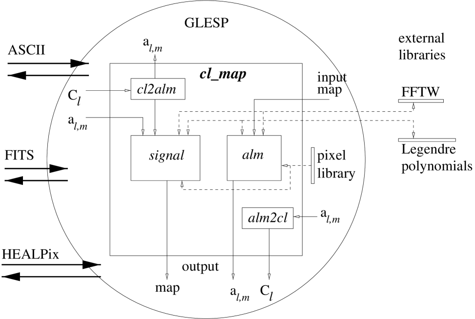
Figure 6: Structure of the GLESP package.

5 Structure of the GLESP code

The code is developed in two levels of organization. The first one, which unifies F77 FORTRAN and C functions, subroutines and wrappers for C routines to be used for FORTRAN calls, consists of the main procedures ’signal’ which transforms given values of $a_{\ell m}$ to a map, ’alm’ which transforms a map to $a_{\ell m}$, ’cl2alm’ which creates a sample of $a_{\ell m}$ coefficients for a given $C_{\ell}$ and ’alm2cl’ which calculates $C_{\ell}$ for $a_{\ell m}$. Procedures for code testing, parameters control Kolmogorov-Smirnov analysis for Gaussianity of $a_{\ell m}$ and homogeneity of phase distribution, and others, are also included. Operation of these routines is based on a block of procedures calculating the Gauss–Legendre pixelization for a given resolution parameter, transformation of angles to pixel numbers and back.

The second level of the package contains the programs which are convenient for the utilization of the first level routines. In addition to the straight use of the already mentioned four main procedures, they also provide means to calculate map patterns generated by the $Y_{20}$, $Y_{21}$ and $Y_{22}$ spherical functions, to compare two sets of $a_{\ell m}$ coefficients, to convert a GLESP map to a HEALPix map, to convert a HEALPix map, or other maps, to a GLESP map

Fig. 6 outlines the GLESP package. The circle defines the zone of the GLESP influence based on the pixelization library. It can include several subroutines and operating programs. The basic program ’cl_map’ of the second level, shown as a big rectangle, interacts with the first level subroutines. These subroutines are shown by small rectangles and call external libraries for the Fourier transform and Legendre polynomial calculations. The package reads and writes data both in ASCII table and FITS formats. More than 10 programs of the GLESP package operate in the GLESP zone.

The present development of the package has also parallel calculation implementation. Visualization procedures in OPEN GL have been developed at IaO, Cambridge.

5.1 Test and precision of the GLESP code

Three tests allow us to check the code. The first of them is from the analytical maps

$$Y_{2,0}=\sqrt{5\over 16\pi}(3x^{2}-1)\,,$$

$$Y_{2,1}=-\sqrt{15\over 8\pi}x\sqrt{1-x^{2}}\cos\phi,\quad$$

$$Y_{2,-1}=-\sqrt{15\over 8\pi}x\sqrt{1-x^{2}}\sin\phi\,,$$

$$Y_{2,2}=\sqrt{15\over 32\pi}(1-x^{2})\cos(2\phi),\quad$$

$$Y_{2,-2}=-\sqrt{15\over 32\pi}(1-x^{2})\sin(2\phi)\,.$$

to calculate $a_{\ell m}$. The code reproduces the theoretical $a_{\ell m}$ better than $10^{-7}$.

The second test is to reproduce an analytical map $\Delta T(x,\phi)=Y_{\ell m}(x,\phi)$ from a given $a_{lm}$ These tests check the calculations of the map and spherical coefficients independently.

The third test is the reconstruction of $a_{\ell m}$ after the calculations of the map, $\Delta T(x,\phi)$, and back. This test allows one to check orthogonality. If the transformation is based on really orthogonal functions it has to return after forward and backward calculation the same $a_{\ell m}$ values.

Precision of the code can be estimated by introduction of a set of $a_{\ell m}=1$ and reconstruction of them. This test showed that using relation (11) we can reconstruct the introduced $a_{\ell m}$ with the precision $\sim 10^{-7}$ limited only by single precision of float point data recording and with the precision $\sim 10^{-5}$ for relation (12).

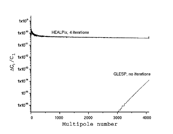
Figure 7: Comparison of calculation accuracy in HEALPix (4 iterations) of the version 1.20 and in GLESP (no iterations) methods. Number of pixels is approximately the same ($\sim 6\times 10^{7}$) and calculation time is proportional to the number of iterations. Note that the comparison is based on iterations of constant signal. For real signal (where $a_{\ell m}\neq$ constant), the accuracy is proportional to the square root of those shown in the figure, i.e. $\Delta C_{\ell}/C_{\ell}<10^{-8}$ for GLESP at $\ell<3000$ whereas $\sim 10^{-5}$ for HEALPix at all multipoles.

Fig. 7 demonstrates the accuracy of $C_{\ell}$ calculations using HEALPix and GLESP.

It should be noted that unlike the HEALPix code, the GLESP method does not needed any iteration for calculation of the $a_{\ell m}$ coefficients and therefore is much faster. Our definition of the $a_{\ell m}$ coefficients is exactly the same as in HEALPix as an estimator of the anisotropy power spectrum:

$$C(\ell)=\frac{1}{2\ell+1}\left[|a_{\ell 0}|^{2}+2\sum_{m=1}^{\ell}|a_{\ell m}|^{2}\right]$$ (26)

5.2 Re-pixelization

Any re-pixelization procedure will cause loss of information and thereby introduce uncertainties and errors. The GLESP code has procedures for map re-pixelization based on two different methods in the $\Delta T(\theta,\phi)$–domain: the first one consists in averaging input values in the corresponding pixel, the second one is connected with spline interpolation inside the pixel grid.

In the first method, we consider input pixels which fell in our pixel with values $\Delta T(\theta_{i},\phi_{i})$ to be averaged with a weighting function. The realized weighting function is a function of simple averaging with equal weights. This method is widely used in appropriation of a given values to the corresponding pixel number.

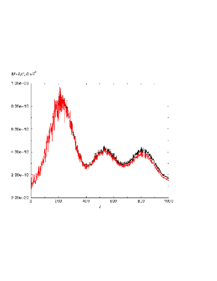
Figure 8: Power spectra calculated for the initial HEALPix map (black curve) with $\ell_{max}=1000$, $N_{side}=1024$, pixel size = 11.8026$\hbox{\hbox to0.0pt{$\sqcap$\hss}$\sqcup$}^{\prime}$, and $N_{tot}$=12 582 912, and for resulting re-pixelized GLESP map (red curve) with the closest possible pixel size = 11.8038$\hbox{\hbox to0.0pt{$\sqcap$\hss}$\sqcup$}^{\prime}$, $N_{tot}$=12 581 579. Deviations of the power spectra at high $\ell$ illustrate the ratio of the HEALPix and GLESP window functions.

In the second method of re-pixelization, we use a spline interpolation approach. If we have a map $\Delta T(\theta_{i},\phi_{i})$ recorded in the knots different from the Gauss–Legendre grid, it is possible to repixelize it to our grid $\Delta T(\theta_{i}^{\prime},\phi_{i}^{\prime})$ using approximately the same number of pixels and the standard interpolation scheme based on the cubic spline approach for the map re-pixelization. This approach is sufficiently fast because the spline is calculated once for one vector of the tabulated data (e.g. in one ring), and values of interpolated function for any input argument are obtained by one call of separate routine (see routines ‘spline’ to calculate second derivatives of interpolating function and ‘splint’ to return a cubic spline interpolated value in Press et al.¹⁴ (1992)).

Our spline interpolation consists of the three steps:

• We set equidistant knots by the $\phi$–axis to reproduce equidistant grid;

• We change grid by $x=\cos\theta$–axis to the required GLESP grid,

• after that, we recalculate $\phi$-knots to the rings corresponding to the GLESP $x$-points.

Fig. 8 demonstrates the deviation of accuracy of the power spectrum in a case of re-pixelization from a HEALPix map to a GLESP map with the same resolution. As one can see, for the range $\ell\leq\ell_{max}/2$, re-pixelization reproduces correctly all properties of the power spectra. For $\ell\geq\ell_{max}/2$ some additional investigations needs to be done to take into account the pixel-window function. This work is in progress.

6 Resume

We suggest a new scheme GLESP for sky pixelization based on the Gauss–Legendre quadrature zeros. It has strict expansion by the orthogonal functions which gives accuracy for $a_{\ell m}$–coefficients calculations below $10^{-7}$ without any iterations. We realized two approaches for Legendre polynomials calculation using $L$– and $M$–methods of calculation schemes.

Among the main advantages of this scheme are

• a high accuracy in calculation $a_{\ell m}$,

• a high speed because of no iterations,

• an optimal selection of resolution for a given beam size, which means an optimal number of pixels and a pixel size.

A corresponding code has been designed in FORTRAN 77 and C languages for procedures of the CMB sky map analysis.

The $a_{\ell m}$ calculation is the main goal. $a_{\ell m}$-s are used in component separation methods and tests for non-Gaussianity (Chiang et al.¹⁰ 2003; Naselsky et al.^11,12 2003b, 2004). It is oriented on the fast and accurate calculation of the $a_{\ell m}$ for the given resolution specified by the beam size. Using accurately calculated $a_{\ell m}$-s, one can reproduce any pixelization scheme by the given pixel centers: GLESP, HEALPix, Igloo or Icosahedron.

Acknowledgments. This paper was supported in part by Danmark Grundforskningsfond through its support for the establishment of the Theorical Astrophysics Center. Authors are thankful to Vladislav Stolyarov for testing parallel capabilities and OPEN GL visualization tool for current pre-release version of GLESP. OVV thanks the RFBR for partial support of the work through its grant 02–07–90038. Some of the results in this paper have been derived using the HEALPix package (Górski, Hivon, and Wandelt⁶ 1999).

References

- (1) [1] Chan, F.K., & O’Neil, E.M., Feasibility study of a quadrilateralized spherical cube Earth data base, Computer Sciences Corp., EPRF Technical Report, 1976.
- (2) [2] O’Neil, E.M., & Laubscher, R.E., Extended studies of a quadrilateralized spherical cube Earth data base, Computer Sciences Corp., EPRF Technical Report, 1976.
- (3) [3] Greisen, E.W. & Calabretta, M., Bull. American Astron. Soc. 182, 09.01 (1993).
- (4) [4] Tegmark, M., ApJL, 470, 81 (1996).
- (5) [5] Crittenden, R.G., & Turok, N.G., 1998, Exactly Azimuthal Pixelizations of the Sky, Report-no: DAMTP-1998-78, 1998 (astro-ph/9806374).
- (6) [6] Górski, K.M., Hivon, E., & Wandelt, B.D., in “Evolution of Large–Scale Structure: from Recombination to Garching”, 1999 (http://www.eso.org/science/healpix).
- (7) [7] Hivon, E., Górski, K.M., Netterfield, C.B., Crill, B.P., Prunet, S., & Hansen, F., ApJ, 567, 2 (2002).
- (8) [8] Stolyarov, V., Hobson, M.P., Ashdown, M.A.J., & Lasenby, A.N., MNRAS, 336, 97 (2002).
- (9) [9] Naselsky, P.D., Verkhodanov, O.V., Chiang, L.-Y., & Novikov, I.D., Submitted to ApJ, 2003a (astro-ph/0310235).
- (10) [10] Chiang, L.-Y., Naselsky, P.D., Verkhodanov, O.V., Way, M.J, 2003, ApJL, 590, 65 (2003).
- (11) [11] Naselsky, P.D., Doroshkevich, A.G., & Verkhodanov, O.V, ApJL, 599, 53 (2003b).
- (12) [12] Naselsky, P.D., Doroshkevich, A.G., & Verkhodanov, O.V, MNRAS, 349, 695 (2004).
- (13) [13] Coles, P., Dineen, P., Earl, J., & Wright, D., MNRAS, 350, 989 (2004).
- (14) [14] Press, W.H., Teukolsky, S.A., Vetterling, W.T., & Flannery, B.P., Numerical Recipes in FORTRAN, Second Edition, Cambridge University Press, 1992.
- (15) [15] Gradsteyn, I.S., & Ryzhik I.M., Tables of Intergrals, Series and Products, Sixth Edition, Academic Press, 2000.
- (16) [16] Frigo, M. & Johnson, S.G., 1997, The Fastest Fourier Transform in the West, Technical Report MIT-LCS-TR-728, 1997.