A Quantitative Comparison of SMC, LMC, and Milky Way UV to NIR Extinction Curves

Abstract

We present an exhaustive, quantitative comparison of all of the known extinction curves in the Small and Large Magellanic Clouds (LMC and SMC) with our understanding of the general behavior of Milky Way extinction curves. The $R_{V}$ dependent CCM relationship and the sample of extinction curves used to derive this relationship is used to describe the general behavior of Milky Way extinction curves. The ultraviolet portion of the SMC and LMC extinction curves are derived from archival IUE data, except for one new SMC extinction curve which was measured using HST/STIS observations. The optical extinction curves are derived from new (for the SMC) and literature UBVRI photometry (for the LMC). The near-infrared extinction curves are calculated mainly from 2MASS photometry supplemented with DENIS and new JHK photometry. For each extinction curve, we give $R_{V}=A(V)/E(B-V)$ and $N(HI)$ values which probe the same dust column as the extinction curve. We compare the properties of the SMC and LMC extinction curves with the CCM relationship three different ways: each curve by itself, the behavior of extinction at different wavelengths with $R_{V}$, and behavior of the extinction curve FM fit parameters with $R_{V}$. As has been found previously, we find that a small number of LMC extinction curves are consistent with the CCM relationship, but majority of the LMC and all of the SMC curves do not follow the CCM relationship. For the first time, we find that the CCM relationship seems to form a bound on the properties of all of the LMC and SMC extinction curves. This result strengthens the picture of dust extinction curves exhibit a continuum of properties between those found in the Milky Way and the SMC Bar. Tentative evidence based on the behavior of the extinction curves with dust-to-gas ratio suggests that the continuum of dust extinction curves is possibly caused by the environmental stresses of nearby star formation activity.

1 Introduction

One of the main tools used in the study of dust grain properties is extinction curves, particularly ultraviolet (UV) extinction curves. The UV is where dust extinction is strongest and shows the large variations from region to region in the Milky Way (Witt, Bohlin, & Stecher, 1984; Aiello et al., 1988; Fitzpatrick & Massa, 1990; Clayton, Gordon, & Wolff, 2000), Large Magellanic Cloud (LMC) (Clayton & Martin, 1985; Fitzpatrick, 1986; Misselt, Clayton, & Gordon, 1999), and Small Magellanic Cloud (SMC) (Lequeux et al., 1982; Prèvot et al., 1984; Gordon & Clayton, 1998).

The work of Cardelli, Clayton, & Mathis (1989) found that most of the variation in Milky Way extinction curves could be described by an empirically relationship based on the single parameter $R_{V}=A_{V}/E(B-V)$. This was a major step forward in our understanding of dust properties and was possible only due to the existence in the literature of near-infrared photometry for a subset of stars in the Fitzpatrick & Massa (1990) sample. This allowed Cardelli, Clayton, & Mathis (1989) to determine $R_{V}$ values and transform the Fitzpatrick & Massa (1990) extinction curves to an absolute scale (i.e., normalized to $A_{V}$ instead of $E(B-V)$). These $A_{V}$ normalized curves had variations which were correlated with $R_{V}$ allowing Cardelli, Clayton, & Mathis (1989) to empirically derive the $R_{V}$ dependent CCM relationship. Since the $R_{V}$ value is a rough measure of average dust grain size, this gave a physical basis for the variations in extinction curves. It is worth noting that significant, small deviations from the CCM relationship are seen for individual sightlines (Mathis & Cardelli, 1992).

The one caveat on the result of Cardelli, Clayton, & Mathis (1989) is that the strength of UV dust extinction limits the measurement of UV dust extinction curves to low to moderate reddening sightlines. This results in a significant bias in measured UV extinction curves in the Milky Way to regions surrounding the Sun. In the one of the largest, detailed study of UV dust extinction curves in the Milky Way to date, Fitzpatrick & Massa (1990) presented curves for 78 sightlines and the average distance probed was 1.3 kpc. The CCM relationship was derived from a subset of the Fitzpatrick & Massa (1990) sample and, as such, this relationship might only be valid for dust in our region of the Milky Way. Clayton, Gordon, & Wolff (2000) tested the validity of the CCM relationship for a larger region of the Milky Way by measuring UV extinction curves along very low-density sightlines. The 26 extinction curves in their sample had an average distance of 5.2 kpc. They found that 19 of the 26 extinction curves in their sample were qualitatively consistent with the CCM relationship. The remaining 7 curves had shapes which are not described by the CCM relationship and were qualitatively similar to those seen in the part of the Large Magellanic Cloud (LMC) (Misselt, Clayton, & Gordon, 1999) associated with the LMC2 supershell (near the 30 Dor star formation region). These 7 curves were all clustered in the same region in the sky and this sightline through the galaxy displays evidence for shocked dust (Clayton, Gordon, & Wolff, 2000).

The CCM relationship seems to be a good description of Milky Way extinction curves with a few exceptions. This raises the question: Does the CCM relationship describe the dust outside of the Milky Way? In other words, are the extinction curves in other galaxies quantitatively similar to those in the Milky Way? Only in the Magellanic Clouds can this question be answered as these are the only two galaxies with reliably measured UV extinction curves. A full answer this question requires $R_{V}$ values for all the Magellanic Cloud extinction curves and this has only been possible with the recent release of the 2MASS observations of the Magellanic Clouds. This is the motivation for this paper. Even without all the needed $R_{V}$ measurements, previous work has gone a long way in answering the above question. It was quickly realized with the first few measured extinction curves in the LMC and SMC the that Clouds had curves which were similar to Milky Way curves as well as curves which were quite different. For example, the sightlines towards the LMC star Sk -69 108 (Nandy & Morgan, 1978) and the SMC star AzV 456 (Lequeux et al., 1982) display Milky Way-like extinction curves. On the other hand, sightlines near 30-Dor in the LMC (Clayton & Martin, 1985; Fitzpatrick, 1986) and in the star forming Bar of the SMC (Prèvot et al., 1984) show definite non-Milky Way-like extinction curves especially in their 2175 Å bump and far-UV rise strengths.

In order to move from a qualitative to a quantitative comparison of Magellanic Cloud and Milky Way extinction curves, $R_{V}$ values are needed for each extinction curve. This allows for the normalization of the extinction curves by $A_{V}$ instead of the usual $E(B-V)$ which the Cardelli, Clayton, & Mathis (1989) work proved was vitally important in understanding the true differences between extinction curves. While, the studies of Gordon & Clayton (1998) and Misselt, Clayton, & Gordon (1999) concentrated on deriving all the UV extinction curves possible with International Ultraviolet Explorer (IUE) archival data in the SMC and LMC, respectively, they also presented $R_{V}$ values for a subset of the SMC and LMC curves. Ideally, the $R_{V}$ values for each extinction curve should be derived from near-infrared photometry of both the reddened and comparison stars which make up each curve. This ensures that the measured extinction curve and $R_{V}$ value correspond to the same dust column and both are similarly corrected for foreground Milky Way dust. Due to the paucity of near-infrared photometry for their reddened and (especially) comparison stars, a majority of the $R_{V}$ values presented in Gordon & Clayton (1998) and Misselt, Clayton, & Gordon (1999) were based on assumed near-infrared intrinsic colors. In addition, the reddened stars’ colors were not corrected for Milky Way foreground dust. This interjected a significant error in the $R_{V}$ values. For example, the foreground extinction can be up to 25% of the total extinction for the LMC extinction curves (Misselt, Clayton, & Gordon, 1999). This results in significant differences between $R_{V}$ values reported in these two studies and previous work (Morgan & Nandy, 1982). The release of the 2MASS data for the Magellanic Clouds makes it possible to correctly and accurately compute $R_{V}$ values for all the known extinction curves in the Magellanic Clouds (Gordon & Clayton, 1998; Misselt, Clayton, & Gordon, 1999) using the 2MASS near-infrared photometry of the reddened and comparison stars.

We combine archival International Ultraviolet Explorer (IUE) ultraviolet spectra, optical photometry, and the 2MASS (Skrutskie et al., 1997) and DENIS (Epchtein et al., 1999; Cioni et al., 2000) near-infrared photometry with new Hubble Space Telescope (HST) Space Telescope Imaging Spectrograph (STIS) ultraviolet spectroscopy and optical photometry to derive ultraviolet through near-infrared extinction curves for 24 sightlines in the Magellanic Clouds in §2. In the same section, we also measure the $R_{V}$ and H I column for all 24 extinction curves. In §3, we quantitatively compare Milky Way and Magellanic Cloud extinction curves as well as discuss various average Magellanic Cloud extinction curves and the existence or lack thereof of the 2175 Å bump in the SMC Bar.

2 Data

We present data on all the sightlines in the Magellanic Clouds which have UV extinction curves. The sightlines include 23 based on IUE data which have been published previously (Gordon & Clayton, 1998; Misselt, Clayton, & Gordon, 1999) and one based on STIS data which are published for the first time in this paper. For each sightline, we have gathered UV spectra and optical and near-infrared photometry for both the reddened and comparison stars. From these data, we have constructed UV to near-IR extinction curves using the standard pair method and measured $R_{V}$ and $N(HI)$ values for each sightline.

2.1 Optical and Near-Infrared Photometry

The optical and near-infrared photometry for the reddened and comparison stars is given in Table 1. UBVRI photometric data for all of the SMC stars as well as two of the LMC stars (Sk -67 36 and Sk -68 26), were obtained on observing runs during 1998 August and September, 1999 January, and 2001 August. The data were acquired at the 1.5-m telescope of the Cerro Tololo Inter-American Observatory (CTIO). A C31034A GaAs photomultiplier, UBVRI filter set #3, and the standard photoelectric data acquisition system were used. Extinction and transformation relations, including non-linear transformation relations were applied to the instrumental data. The final magnitudes and color indices are on the photometric system defined by Landolt (1992). The UBV optical photometry for the remainder of the LMC stars was taken from Misselt, Clayton, & Gordon (1999).

The JHK near-infrared photometry for most of the SMC and LMC stars was taken from the results of the 2MASS project (Skrutskie et al., 1997). The JHK photometry for the SMC stars AzV 456 and AzV 462 was taken from Bouchet et al. (1985). For two of the three LMC stars without 2MASS photometry, we used the DENIS (Epchtein et al., 1999; Cioni et al., 2000) JK photometry converted to the 2MASS system (Cutri et al., 2000). For the one LMC star without 2MASS or DENIS photometry due to a nearby saturating star, we used JHK images of Sk -68 26 and its surrounding region which were taken using the Cerro Tololo InfraRed IMager (CIRIM) at the CTIO 1.5m. These images were taken on 15 Dec 1999 in non-photometric weather and each band was observed 4 times offsetting between positions for a total exposure time of 4 seconds. The field-of-view of the coadded images was approximately $200\arcsec\times 200\arcsec$. In this region, 5 of the bright stars have 2MASS observations and we used these stars to calibrate the JHK fluxes for Sk -68 26 using differential photometry. The uncertainty in these measurements was calculated as the standard deviation of the mean of the the 5 measurements of the JHK magnitudes of Sk -68 26, one measurement per 2MASS star.

2.2 Ultraviolet Spectra

The UV spectra for all but two of the stars in this paper were taken from archival IUE observations. The specific IUE observations we used are given by Gordon & Clayton (1998) for the SMC stars and Misselt, Clayton, & Gordon (1999) for the LMC stars. The individual IUE observations were downloaded from the MAST archive at Space Telescope Science Institute (STScI) and were coadded to produce a single spectrum from 1150 to 3225 Å with a resolution of approximately 400. The calibration of these spectra was improved using the results of Massa & Fitzpatrick (2000) who found that the signal-to-noise of IUE low-dispersion data could be significantly improved over that provided in the IUE archive.

Figure 1: The STIS spectra of AzV 23 and 404 are plotted in (a). The resulting extinction curve for AzV 23 is shown in (b). The region near Ly$\alpha$ has been corrected for H I absorption.

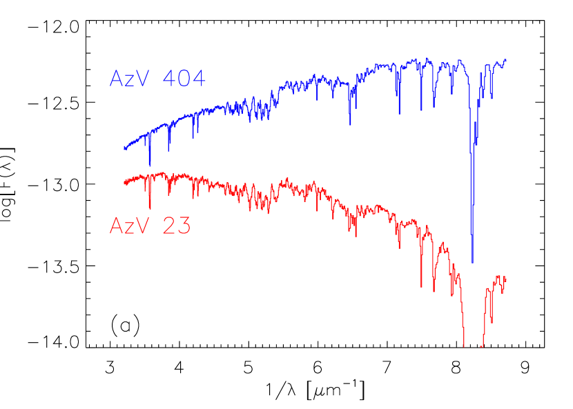
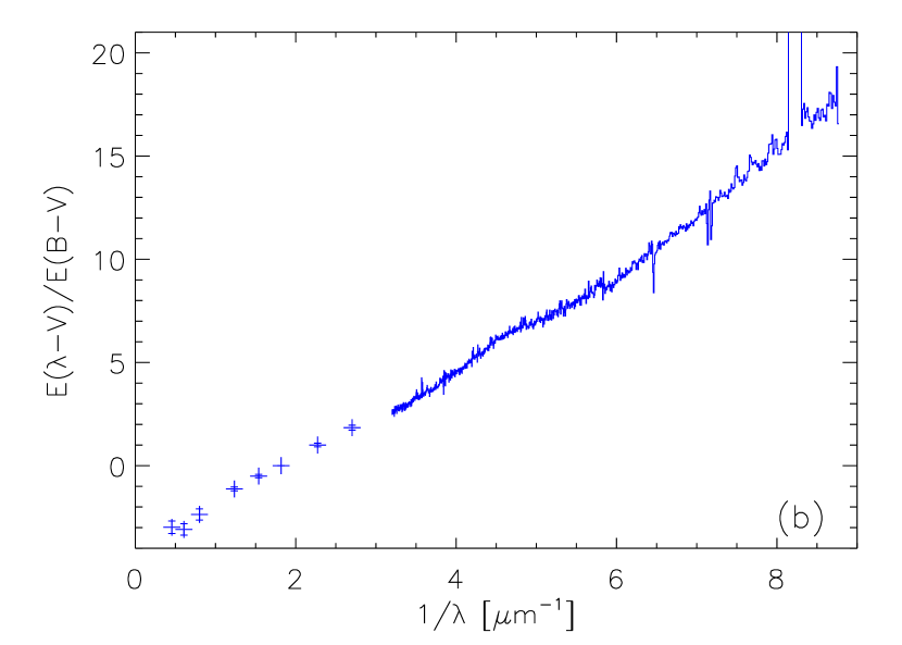
The UV spectra for the final two stars (AzV 23 and 404) were taken with the STIS instrument on HST as part of our GO program #8198. The spectra were taken using the 52x0.5$\arcsec$ slit with the G140L and G230L gratings. The individual observations were coadded to produce spectra extending from 1140 to 3140 Å with a resolution of approximately 1000. These two spectra are presented in Fig. 1. The excellent match between the reddened and comparison spectral types can be easily seen in this figure. In addition, the superior nature of STIS ultraviolet spectra as compared to IUE spectra can be seen by comparing this figure with Fig. 1 of Gordon & Clayton (1998) which displays IUE spectra for similar spectral type stars.

2.3 Extinction Curves

The extinction curves for sightlines in the Magellanic Clouds were derived using the standard pair method. The reddened/comparison star pairs used are listed in Table 2. We rederived the 23 extinction curves presented in Gordon & Clayton (1998) and Misselt, Clayton, & Gordon (1999) to take into account the new calibration of IUE low-dispersion data (Massa & Fitzpatrick, 2000) and the new optical and near-infrared photometry. The effects of the new calibration of the IUE spectra on the UV extinction curves was small, mainly reducing the noise in the curves. The one new extinction curve in the SMC for the AzV 23 sightline is presented in Fig. 1 at it’s full spectral resolution.

Figure 2: The SMC extinction curves are plotted. The best fit FM90 curve (solid line) and its uncertainties are plotted (dashed lines). The CCM curve for the measured $R_{V}$ value (dotted line) and its uncertainties (dot-dashed lines) are plotted.

Figure 3: The LMC extinction curves in the LMC-2 sample are plotted. The best fit FM90 curve (solid line) and its uncertainties are plotted (dashed lines). The CCM curve for the measured $R_{V}$ value (dotted line) and its uncertainties (dot-dashed lines) are plotted.

Figure 4: The LMC extinction curves in the LMC-average sample are plotted. The best fit FM90 curve (solid line) and its uncertainties are plotted (dashed lines). The CCM curve for the measured $R_{V}$ value (dotted line) and its uncertainties (dot-dashed lines) are plotted.

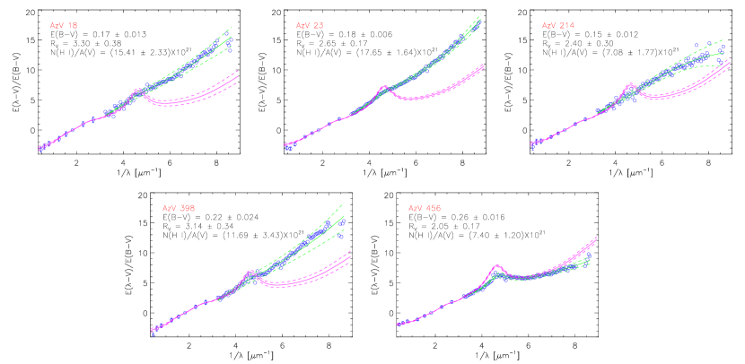
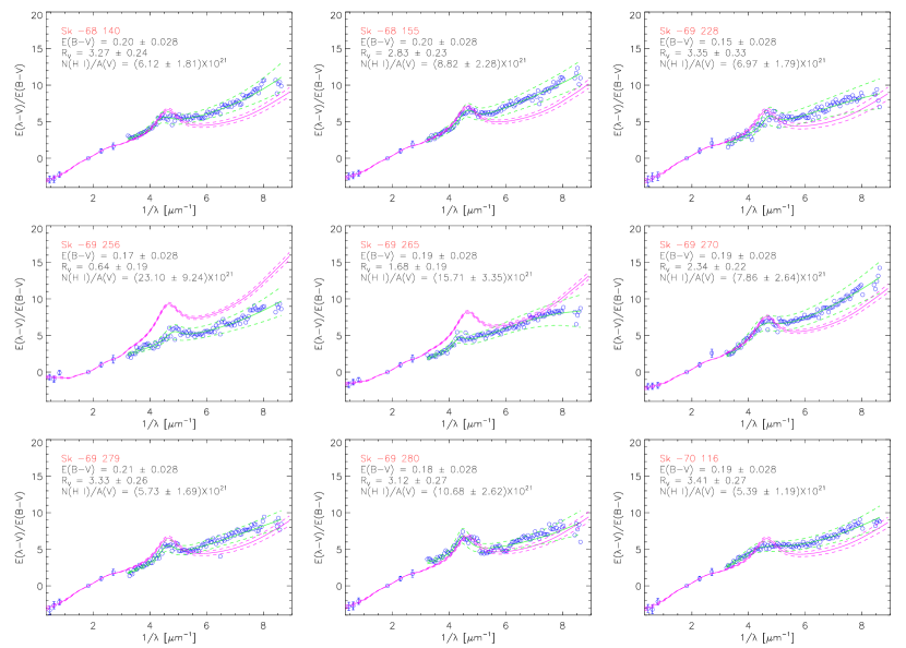
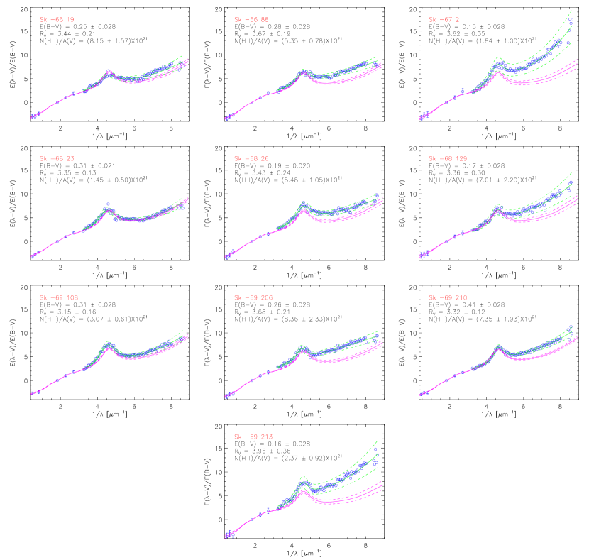
We calculated all 24 extinction curves and their associated uncertainties as outlined in Gordon & Clayton (1998). In addition, we removed the effects of the Ly$\alpha$ H I absorption using our measurements of the H I column (see §2.6). These extinction curves give the difference in extinction between the two sightlines to the reddened and comparison stars. The Milky Way foreground component is effectively removed as long as the reddening due to this component towards the reddened and comparison star pairs are similar (Misselt, Clayton, & Gordon, 1999). This results in an extinction curve that only measures dust in the Magellanic Clouds. All 24 extinction curves are plotted in Figs. 2-4.

2.4 FM Parameters

We fit each curve with the FM parameterization of the shape of the UV extinction curve (Fitzpatrick & Massa, 1990). The FM parameterization is

$$E(x-V)/E(B-V)=C_{1}+C_{2}x+C_{3}D(x,\gamma,x_{o})+C_{4}F(x)$$ (1)

where $x=\lambda^{-1}$,

$$D(x,\gamma,x_{o})=\frac{x^{2}}{(x^{2}-x_{o}^{2})^{2}+x^{2}\gamma^{2}},$$ (2)

and

$$F(x)=0.5392(x-5.9)^{2}+0.05644(x-5.9)^{3}$$ (3)

for $x\geq 5.9$ and $F(x)=0$ for $x<5.9$. We determined the FM parameters for the extinction curves by numerically minimizing the $\chi^{2}$ in a manner similar to that used by Fitzpatrick & Massa (1990). First, $x_{o}$ and $\gamma$ were fixed and the values of $C_{1}$, $C_{2}$, $C_{3}$, and $C_{4}$ were determined by minimizing the $\chi^{2}$. Next, $C_{1}$, $C_{2}$, $C_{3}$, $C_{4}$, and $\gamma$ were fixed and the value of $x_{o}$ was determined by minimizing the $\chi^{2}$. Finally, $C_{1}$, $C_{2}$, $C_{3}$, $C_{4}$, and $x_{o}$ were fixed and the value of $\gamma$ was determined by minimizing the $\chi^{2}$. These two steps were repeated until the $\chi^{2}$ no longer changed by a significant amount. This three step method gives a smaller $\chi^{2}$ than doing a single $\chi^{2}$ minimization while simultaneously fitting all 6 parameters. It is worth noting that there are probably only 5 independent parameters in the FM equation. While all evidence points to $C_{1}$ and $C_{2}$ being correlated in the Milky Way and the Magellanic Clouds (Fitzpatrick & Massa, 1988; Misselt, Clayton, & Gordon, 1999), we have not assumed this correlation.

For the 4 SMC Bar extinction curves, we set $x_{o}=4.6$ and $\gamma=1.0$ as the weak to nonexistent 2175 Å bumps in these curves precludes fitting all three bump parameters. This allows for a more realistic measurement of the bump strength or an upper limit for these weak bump sightlines.

The uncertainties in the FM parameters for low $E(B-V)$ sightlines are dominated by the uncertainty in $E(B-V)$ and the random uncertainties of each wavelength point. The uncertainties in the extinction curves were calculated using eq. 2 of Gordon & Clayton (1998). From this equation, it can be seen that an uncertainty in $E(B-V)$ affects the extinction curve in a correlated way. Uncertainties in $E(B-V)$ do not add random noise to each wavelength point, but shift the entire extinction curve up and down. The random uncertainties at each wavelength point contribute a smaller uncertainty, except in the case of $x_{o}$ and $\gamma$. The contribution of uncertainties in $E(B-V)$ ($\sigma[E(B-V)]$) to the FM parameter uncertainties were calculated by fitting the two additional curves for each measured extinction curve which describe the effects of the $E(B-V)$ uncertainty. These curves are $\left(1+\sigma E(B-V)/E(B-V)\right)E(x-V)/E(B-V)$ and $\left(1-\sigma E(B-V)/E(B-V)\right)E(x-V)/E(B-V)$. The $E(B-V)$ uncertainties in each FM parameter were then one half the difference between the parameters for these two curves.

The FM parameter uncertainties due to the random uncertainties ($\sigma(random)$) were calculated using a Monte Carlo approach. Determining the random component of the FM parameter uncertainties is not usually done, but we found that the random component dominates the $x_{o}$ and $\gamma$ uncertainties. This method consisted of generating 100,000 possible FM fits similar to the best FM fit and determining which ones fit equally well within $3\sigma$ using the F-test where the $\sigma$ is only that due to random flux uncertainties. The resulting $1\sigma(random)$ uncertainties were determined by dividing by three. The reported FM uncertainties (see Table 3) were determined by summing in quadrature the $E(B-V)$ associated ($\sigma[E(B-V)]$) and random ($\sigma(random)$) uncertainties. The $E(B-V)$ uncertainties dominate the $C_{1}$, $C_{2}$, $C_{3}$, and $C_{4}$ uncertainties, while the random uncertainties dominate the $x_{o}$ and $\gamma$ uncertainties.

2.5 $R_{V}$ values

The value of $R_{V}=A_{V}/E(B-V)$ for each sightline was determined using a $\chi^{2}$ minimization method. This method relies on the invariance of the RIJHK portion of the extinction curve (Rieke & Lebofsky, 1985; Martin & Whittet, 1990). The $R_{V}$ value for each extinction curve is the value which minimizes the $\chi^{2}$ between the measured RIJHK extinction and the Rieke & Lebofsky (1985) curve. The equation giving $\partial\chi^{2}/\partial R_{V}=0$ was solved and the analytic solution for $R_{V}$ was found. From this equation, the uncertainty for $R_{V}$ was derived. See the appendix for details of this derivation. The $R_{V}$ values and uncertainties are tabulated in Table 2. Our method of using the RIJHK extinction curve itself to determine $R_{V}$ values is different from what is usually done. Usually the observed VRIJHK or just VK photometry of the reddened star is compared to assumed intrinsic colors (Morgan & Nandy, 1982; Cardelli, Clayton, & Mathis, 1989; Gordon & Clayton, 1998; Misselt, Clayton, & Gordon, 1999). In the Magellanic Clouds, the reddened stars are usually first corrected for the average Milky Way foreground reddening (Morgan & Nandy, 1982). Instead, we have used the measured VRIJKH photometry for the matched comparison star and avoided having to assume intrinsic colors of the reddened star. This naturally removes the foreground Milky Way reddening and ensures that the measured $R_{V}$ value corresponds to the same dust column as the extinction curve. The CCM relationship for these $R_{V}$ values for each measured extinction curve is given in Figs. 2-4. The effects of the uncertainty in $R_{V}$ on the CCM relationship is shown in these plots using dashed curves.

2.6 H I columns

Figure 5: The ratio spectra for the AzV 23/404 pair (a) and Sk -69 108/Sk -67 78 pair (b) are shown (solid line) with the best fit H I profile (dot-dashed line). The ratio spectrum divided by the best fit model Ly$\alpha$ profile is shown as a dashed line. The vertical dotted lines give the center of the Ly$\alpha$ line for the SMC (a) and LMC (b) velocities and $\pm 12$Å region which is excluded from the fit. The dotted line gives a nominal continuum.

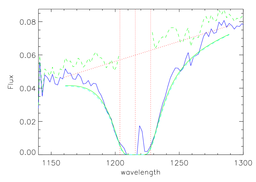
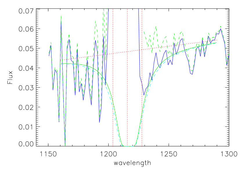
We determined the H I column for each extinction curve using a variant of the method outlined in Bohlin (1975). This method relies on fitting the wings of the Ly$\alpha$ absorption profile. As we are only interested in a measurement of the difference in the H I column between the reddened and comparison stars, we made this measurement in the ratio spectrum for each reddened and comparison star pair. The uncertainty in this measurement was estimated by eye, varying the H I value until it was noticeable incorrect. Two examples of this are shown in Fig. 5. Basically, the strength of a model Ly$\alpha$ profile is adjusted until the division of the ratio spectrum by the model spectrum yields a straight line. The central wavelength of the Ly$\alpha$ line for the LMC and SMC is corrected for the heliocentric velocity of the LMC and SMC (280 and 130 km/s, respectively). The central region of the Ly$\alpha$ line is ignored as it is contaminated by geocoronal emission. This measurement is straightforward for the STIS data. For IUE data, this measurement is much more uncertain as the contamination by geocoronal emission is much larger and the spectra blueward of Ly$\alpha$ are very noisy. The red wing of Ly$\alpha$ was mainly used in the measurement of H I columns for the IUE data. The measured H I values and uncertainties are tabulated in Table 2.

3 Discussion

3.1 Comparison of Magellanic Cloud and Milky Way Extinction Curves

Now that we have produced full ultraviolet to near-infrared extinction curves (in units of $A(\lambda)/A(V)$) for all the known Magellanic Cloud reddened/comparison star pairs, we can quantitatively compare them to Milky Way extinction curves. The $R_{V}$ dependent CCM relationship and the CCM sample extinction curves provides a nice, compact form for representing the properties of Milky Way dust found in the local interstellar medium. Thus, we can compare Milky Way and Magellanic Clouds dust by seeing if the CCM relationship is applicable to any of the individual extinction curves or describes aspects of the sample behavior of these curves.

To test if the CCM relationship accurately describes any of the individual extinction curves, we compare the full measured UV to NIR extinction curves to the appropriate CCM curve for the measured $R_{V}$. This is done in Figs. 2-4 and includes curves showing the uncertainty in the measured curve as well as the uncertainty in the CCM curve due to uncertainty in the measured $R_{V}$ value. It should be remembered that the CCM relationship gives the average behavior at a particular $R_{V}$ and that individual curves can have small deviations from this average behavior and still follow the CCM relationship.

It is clear from Fig. 2 that the four curves located in the star-forming bar of the SMC (AzV 18, 23, 214, & 398) do not follow the CCM relationship. For the one curve located outside of the SMC bar (AzV 456), the CCM curve does a better job following the measured curve, but there still are significant deviations at the 2175 Å bump and in the far-UV ($>7\micron^{-1}$). Thus, there are no measured extinction curves in the SMC which follow the CCM relationship.

In the LMC, there is one curve in the LMC2 sample (Sk -69 280) and three curves in the LMC-average sample (Sk -66 19, Sk -68 23, & Sk -69 108) which follow the CCM relationship within their uncertainties (Figs. 3-4). Thus, there is evidence that the CCM relationship is at work in the LMC, but only in a limited sense as it describes only 4 out of the 19 measured extinction curves.

Figure 6: Plots of $A_{\lambda}/A_{V}$ versus $R_{V}^{-1}$ are shown where $A_{12}=A(1200$ Å), $A_{15}=A(1500$ Å), $A_{22}=A(2200$ Å), $A_{28}=A(2800$ Å), $A_{U}=A(3500$ Å, U band), $A_{J}=A(1.25$ µm, J band). The LMC and SMC measurements are given by the circles (solid = Average and open = LMC2) and squares (solid = Bar and open = Wing) with error bars, respectively. The line gives the CCM relationship and the open circles without error bars the original Fitzpatrick & Massa (1990) data used by CCM ($\lambda<3000$ Å plots only).

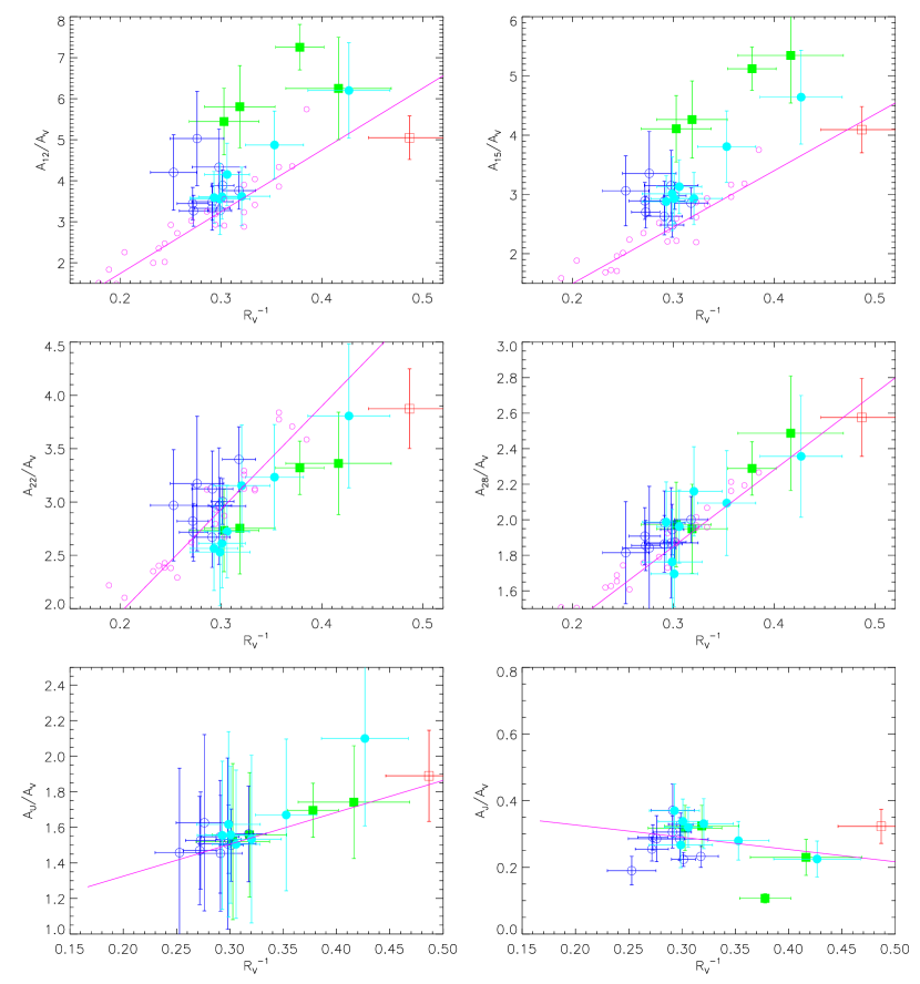
The most direct way to quantify how applicable the CCM relationship is in the Magellanic Clouds is to plot $R_{V}^{-1}$ versus $A_{\lambda}/A_{V}$. This was how the CCM relationship was originally presented by Cardelli, Clayton, & Mathis (1989). Fig. 6 shows such plots for $\lambda=$ 1200, 1500, 2200, & 2800 Å and U and J bands. Since the CCM relationship represents the average extinction behavior as a function of $R_{V}$, saying extinction measurements do not follow CCM is to say that they are beyond the scatter of the extinction curves which were used to derive the CCM relationship. In Fig. 6, the small open circles without error bars give data for the extinction curves used to derive CCM and can be used to determine the scatter which is consistent with the CCM relationship. These plots show that at far-UV wavelengths ($\lambda=$ 1200 & 1500 Å) the CCM relationship forms a lower bound to the values of $A(\lambda)/A(V)$ at a particular value of $R_{V}$. At longer wavelengths ($\lambda\geq 2200$ Å), the Magellanic Clouds measurements are indistinguishable from the CCM relationship within their uncertainties.

Figure 7: The FM fit parameters are plotted versus $R_{V}^{-1}$. The LMC and SMC measurements are given by the circles (solid = Average and open = LMC2) and squares (solid = Bar and open = Wing) with error bars, respectively. The line gives the CCM relationship and the open circles without error bars the original Fitzpatrick & Massa (1990) data used by CCM.

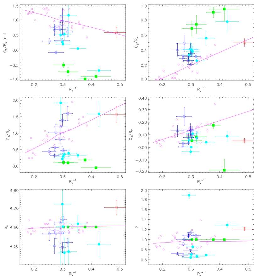
A final way to probe how well the CCM relationship works in the Magellanic Clouds is to examine behavior of the FM parameters as a function of $R_{V}$. The FM parameters describe the UV extinction curve with only 6 parameters allowing for more sensitive tests to be performed. The FM parameters $C_{1}$, $C_{2}$, $C_{3}$, and $C_{4}$ have a factor of $R_{V}$ embedded in them, we have plotted the equivalent $R_{V}$-independent coefficients versus $R_{V}^{-1}$ in Fig. 7. These $R_{V}$-independent coefficients can be derived by examining eq. 1 converted from $E(x-V)/E(B-V)$ to $A(x)/A(V)$ units. The equation expressed this way is

$$A(x)/A(V) = \frac{E(x-V)}{E(B-V)}\frac{1}{R_{V}}+1$$ (4)

$$= (C_{1}/R_{V}+1)+(C_{2}/R_{V})x+(C_{3}/R_{V})D(x,\gamma,x_{o})+(C_{4}/R_{V})F(x).$$ (5)

The behavior of the $(C_{1}/R_{V}+1)$, $C_{2}/R_{V}$, $C_{3}/R_{V}$, and $C_{4}/R_{V}$ coefficients do not follow the CCM relationship directly, but the CCM relationship does form a bound on the values of these coefficients as a function of $R_{V}$. For example, all the values of $C_{2}/R_{V}$ lie on or above the line defining the CCM relationship. In the plots of the other three coefficients, the CCM relationship forms an upper bound on their behaviors. In the case of $x_{o}$ and $\gamma$, CCM does not predict much of a dependence on $R_{V}$ and we do not see one for the Magellanic Clouds either. The values of $x_{o}$ and $\gamma$ for the Magellanic Clouds have a much larger scatter than seen in the extinction curves defining CCM. For $x_{o}$ this scatter is consistent with the uncertainties in $x_{o}$. For $\gamma$, the scatter is larger than can be accounted for by measurement uncertainties. Thus, it is either real or the result of measurement uncertainties we have not accounted for in our error analysis.

By examining the behavior of the Magellanic Cloud extinction curves with $R_{V}$ three different ways and comparing that behavior to that predicted by the $R_{V}$ dependent CCM relationship, we find evidence that the general behavior of Milky Way extinction curves is seen in the Magellanic Clouds. Not only are 4 LMC extinction curves indistinguishable from Milky Way extinction curves, but the general behavior of Milky Way extinction curves forms a bound on the general behavior of Magellanic Cloud extinction curves.

3.2 Super-CCM relationship?

While a small number of Magellanic Cloud extinction curves do seem to be well described by the CCM relationship, the majority do not. Yet there is strong evidence that the CCM relationship serves as a bound on the behavior of all the Magellanic Cloud extinction curves. This fact raises the question: Is there some more general relationship dependent on $R_{V}$ and at least one other parameter which describes the average behavior of the Milky Way and Magellanic Cloud extinction curves?

Figure 8: The strength of the 2175 Å bump ($A(bump)/A(V)=C_{3}/(\gamma^{2}R_{V})$) is plotted versus the steepness of the ultraviolet extinction ($C_{2}/R_{V}$). The LMC and SMC measurements are given by the circles (solid = Average and open = LMC2) and squares (solid = Bar and open = Wing) with error bars, respectively. The line gives the CCM relationship and the open circles without error bars the original Fitzpatrick & Massa (1990) data used by CCM.

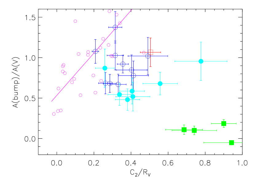
An indication that such a relationship might exist was presented by Clayton, Gordon, & Wolff (2000) for low density sightlines in the Milky Way which display some of the same deviations from CCM seen in the Magellanic Clouds. They found that the strength of the 2175 Å bump ($(\pi C_{3})/(2\gamma)$) and the steepness of the ultraviolet extinction ($C_{2}$) were anti-correlated along the low density sightlines as well as for the average curves in the Magellanic Clouds (Gordon & Clayton, 1998; Misselt, Clayton, & Gordon, 1999). We present a similar plot in Fig. 8 for the Magellanic Cloud extinction curves with the equivalent $R_{V}$ independent measures of the 2175 Å bump strength and ultraviolet extinction steepness. This plot gives evidence for an anti-correlation between the strength of the 2175 Å bump and the steepness of the ultraviolet extinction.

Figure 9: The behavior of the gas-to-dust ratios ($N(HI)/A(V)$) versus (a) 2175 Å bump strength ($A(bump)/A(V)$) and (b) ultraviolet steepness ($C_{2}/R_{V}$) is shown. The LMC and SMC measurements are given by the circles (solid = Average and open = LMC2) and squares (solid = Bar and open = Wing) with error bars, respectively. The line gives a simple linear fit to the data.

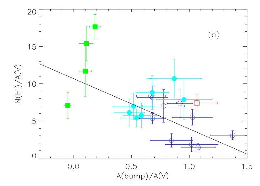
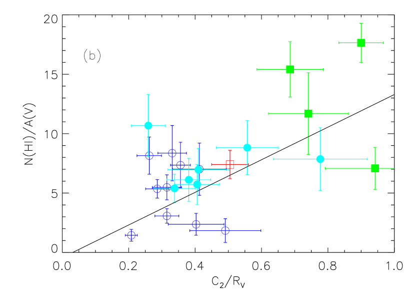
One possible second parameter could be the measured gas-to-dust ratio ($N(HI)/A(V)$). To test this we have plotted in Fig. 9 the gas-to-dust ratios versus the 2175 Å bump strength and ultraviolet steepness values for the Magellanic Cloud extinction curves. The scatter in these two plots is quite large as are the uncertainties on the individual points. There might be real correlations in both plots, but higher quality data are needed. There would be reason to expect a correlation between the gas-to-dust ratio and the behavior of extinction curves. The gas-to-dust ratio is known to correlate with metallicity on a galaxy wide basis (Issa, MacLaren, & Wolfendale, 1990). On a local scale, it could be a measure of the formation and destruction history of dust grains. For example, the dust self-shielding will decrease with increasing gas-to-dust ratio making it easier for dust grains to be destroyed by the ambient radiation field. If the dust grains responsible for the 2175 Å bump are easier to destroy than those responsible for the underlying ultraviolet extinction, a behavior like that seen in Fig. 9 would be expected.

3.3 SMC Bar extinction curves and the 2175 Å bump

The extremely weak or absent 2175 Å bump in the four SMC Bar extinction curves makes these curves unique. In all other measured extinction curves, the 2175 Å bump is quite prominent. The obvious question is whether the weak 2175 Å bump in the SMC Bar is due to Milky Way contamination or is intrinsic to the SMC. While only one of the four curves has a bump which is detected at greater than $3\sigma$, the other three are all $2\sigma$ detections. The construction of the curves using SMC comparison stars should remove all the Milky Way foreground, but small differences between the reddened and comparison stars foreground could result in a weak 2175 Å bump. A foreground contamination like this would result in a positive bump as often as a negative bump. Interestingly, one out of the four SMC Bump curves (AzV 214) has a $2\sigma$ detection of a negative bump and a negative far-UV curvature ($C_{4}$). The foreground contamination (in percent of total $E(B-V)$ with $1\sigma$ uncertainties) needed to produce spurious bump detections at the observed levels would have to be ($25\pm 14$)%, ($39\pm 10$)%, ($10\pm 5$)%, and ($23\pm 13$)% for AzV 18, 23, 214, and 398, respectively. These foreground contaminations are not unlikely given the low $E(B-V)$ values for these sightlines, especially given the large uncertainties. While it is difficult to definitively decide, the current evidence suggests that the carriers of the 2175 Å bump could be completely absent from the dust in the SMC Bar sightlines.

3.4 Sample Average Curves

Since the Magellanic Cloud extinction curves display significantly different shapes than that seen in the Milky Way, average extinction curves of the LMC-average, LMC2-supershell, and SMC-Bar samples are of interest. These average curves capture the large scale variations in dust properties at higher signal-to-noise than the individual curves.

Figure 10: The sample average extinction curves are plotted along with the “average” Milky Way curve (CCM with $R_{V}=3.1$).

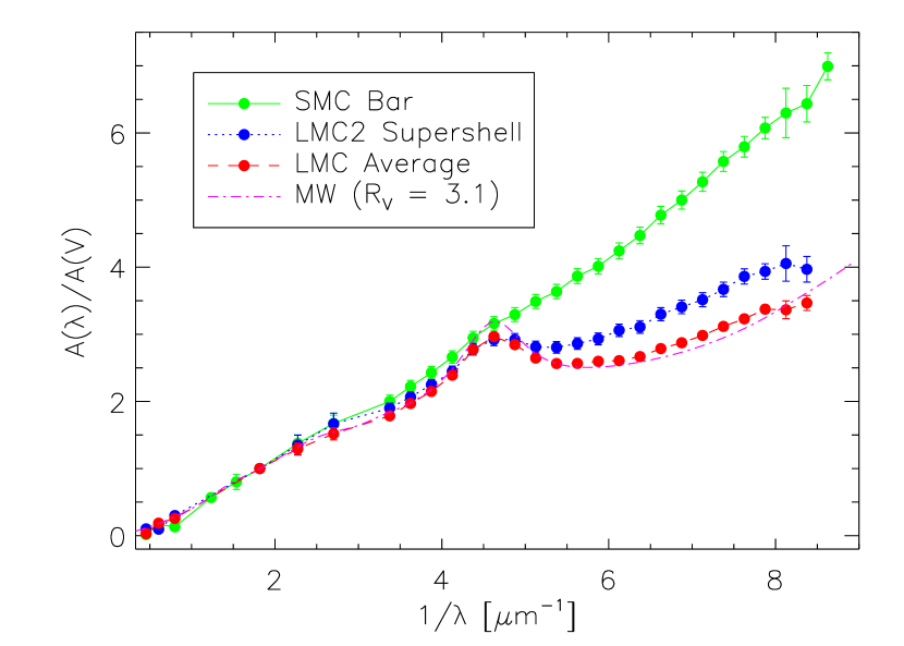
While past work has produced such average curves (Gordon & Clayton, 1998; Misselt, Clayton, & Gordon, 1999), we can create more accurate average curves as the result of our determinations of $R_{V}$ values. We have averaged the individual curves in each sample in $A(\lambda)/A(V)$ units instead of $E(\lambda-V)/E(B-V)$ units as was done in previous work. $E(\lambda-V)/E(B-V)$ units are a relative measure of dust properties whereas $A(\lambda)/A(V)$ units are an absolute measure of the dust properties and, as a result, more accurately represent the effects of dust. For the LMC2 supershell sample, we have not used the results for Sk -69 256 in producing the LMC2 supershell average. It’s extremely low $R_{V}$ value of $0.64$ is likely the result of poor JHK photometry, contamination by nearby hot dust, or contamination by a red companion.

The sample average curves are given in Figure 10 and tabulated in Table 4. The averages were calculated weighting by the uncertainties at each wavelength for each individual curve and in 0.25 $\micron^{-1}$ wide bins. The average values of $R_{V}$ and N(H I)/A(V) were also calculated weighting by the individual uncertainties and are tabulated in Table 2. The average curves were fit with the FM parameterization and the best fit 6 FM parameters are given in Table 3. The FM fits were done for wavelengths $<8.4$ $\micron$ as this is the bluest wavelength in common between the IUE and STIS data. This fitting limit only affected the SMC Bar average.

For the SMC Bar, we find that $R_{V}=2.74\pm 0.13$ and N(H I)/A(V) $=13.18\pm 1.02$ which is consistent with the results of Bouchet et al. (1985) and Gordon & Clayton (1998). However, we do not find that the gas-to-dust ratio for AzV 456 (Sk 143) is similar to that of the Milky Way. For the Milky Way, N(H I)/A(V) $\sim 1.55$ (Bohlin, Savage, & Drake, 1978; Diplas & Savage, 1994) and we find N(H I)/A(V) $=7.40\pm 1.20$ for AzV 456 whereas Bouchet et al. (1985) found N(H I)/A(V) $\sim 2.6$ assuming $R_{V}=2.72$ (the average $R_{V}$ for the entire SMC). The differences between our measurement and Bouchet et al. (1985) can be traced to our lower $E(B-V)$ and a lower $R_{V}$ value. These differences illustrate the difficulties of measuring such quantities for low reddening sightlines.

For the LMC2 supershell sample, we find that $R_{V}=2.76\pm 0.09$ and N(H I)/A(V) $=6.97\pm 0.67$. Our gas-to-dust ratio is roughly consistent with results of Koornneef (1982) and Fitzpatrick (1985) who found N(H I)/A(V) $\sim 6.3$ and $8.7$, respectively. Our value of $R_{V}$ is lower than that of Clayton & Martin (1985) who found $R_{V}\sim 3.5$ but consistent with Misselt, Clayton, & Gordon (1999). For the LMC average sample, we find that $R_{V}=3.41\pm 0.06$ and N(H I)/A(V) $=3.25\pm 0.28$. These values are significantly different from those for the LMC2 supershell sample. The different gas-to-dust ratios is in conflict with the conclusions of Fitzpatrick (1986) who state that there are no gas-to-dust measurable differences between the non-30 Dor and 30 Dor samples. But, examination of their Fig. 6 shows that the non-30 Dor points fall consistently below 30 Dor gas-to-dust ratio implying that we are not in conflict with earlier work. The lower gas-to-dust ratio is especially interesting as it supports a systematic trend of more extreme extinction curves (smaller 2175 Å bump and steeper far-UV rise) with rising gas-to-dust ratio (see §3.2).

4 Conclusions

We have presented a quantitative, exhaustive comparison of all the known Magellanic Cloud extinction curves with a representative sample of Milky Way extinction curves. Like previous studies (Nandy & Morgan, 1978; Lequeux et al., 1982; Prèvot et al., 1984; Clayton & Martin, 1985; Fitzpatrick, 1986; Gordon & Clayton, 1998; Misselt, Clayton, & Gordon, 1999) we find that both the LMC and SMC have examples of extinction curves qualitatively similar to those found in the Milky Way. Unlike previous studies, we are able to take this comparison one step further and make quantitative comparisons as we determined $R_{V}$ values for all Magellanic Cloud extinction curves. This allows for the comparison of Magellanic Cloud and Milky Way extinction curves to be done using measurements based on absolute dust properties ($A(\lambda)/A(V)$) instead of relative dust properties ($E(\lambda-V)/E(B-V)$). The importance of this difference is well illustrated by the work of Cardelli, Clayton, & Mathis (1989) where the comparison of Milky Way curves in $A(\lambda)/A(V)$ units allowed for the derivation of the $R_{V}$ dependent CCM relationship. We conclude that 4 extinction curves in the LMC are indistinguishable from Milky Way extinction curves and Milky Way extinction curves form a bound on the behavior of Magellanic Cloud extinction curves.

The majority of the Magellanic Cloud extinction curves are significantly different than Milky Way extinction curves and this is likely a result of Magellanic Cloud extinction curves probing quite different environments than the CCM sample of Milky Way extinction curves. The CCM sample is based on fairly quiescent sightlines and most of our extinction curve measurements in the Magellanic Clouds are biased towards quite active regions as they are based on OB supergiants. The systematic behavior of the curves studied in this paper hint at the existence of a multiparameter relationship (possibly dependent on $R_{V}$ and $N(HI)/A(V)$) describing both quiescent (CCM-like) and active extinction curves.

The different biases between the majority of the measured Milky Way and Magellanic Cloud extinction curves point to a weakness in our understanding of dust properties. The Magellanic Cloud extinction curves are biased towards active star forming regions (OB supergiant sightlines) and low dust columns. The Milky Way sightlines are less biased towards active star forming regions as they are mainly measured along sightlines towards OB main sequence stars. They are limited in their variety of dust properties probed as the measurements are generally limited to our local region of the Milky Way. Evidence that the type of dust seen in the Magellanic Clouds does exist in the Milky Way is seen along Milky Way low density sightlines (Clayton, Gordon, & Wolff, 2000). Higher dust column sightlines and sightlines towards main sequence stars need to be measured in the Magellanic Clouds to allow us to truly explore the possible range of dust properties.

The results of this work and those of Clayton, Gordon, & Wolff (2000) imply that the common usage of discussing Milky Way, LMC, and SMC dust as separate is inaccurate. In reality, a continuum of dust properties exists between that seen in the quiescent and active regions (eg., see Fig. 8). The usual average curves can then be arranged into a rough version of this sequence and it would be Milky Way (CCM) – LMC Average – SMC Wing (AzV 456) – LMC2 Supershell – SMC Bar. Ordering all the individual known extinction curves would produce an even greater mixing of Milky Way, LMC, and SMC curves. This work describes a qualitative view of the continuum of dust extinction curves. Quantifying the variation between quiescent and active region extinction curves would give valuable clues to the identities of dust grain properties.

Appendix A $R_{V}$ value and uncertainty equations

The derivation of the equations to determine value of $R_{V}$ and its uncertainty are given in this appendix. To the knowledge of the authors, these equations have not appeared in the literature before and are included in this paper as they may be of use to others. The equations below are equivalent to determining $R_{V}$ from individual colors and averaging the results weighted by the appropriate uncertainties.

The equation giving the $\chi^{2}$ between the measured extinction curve and the Rieke & Lebofsky (1985) curve is

$$\chi^{2}=\sum_{i}\left[\frac{y(\lambda_{i})-y(R_{V},\lambda_{i})}{\sigma(\lambda_{i})}\right]^{2}$$ (A1)

where

$$y(\lambda_{i}) = E(\lambda_{i}-V)/E(B-V)$$ (A2)

$$\sigma(\lambda_{i}) = \sigma E(\lambda_{i}-V)/E(B-V)$$ (A3)

$$y(R_{V},\lambda_{i}) = \left[A(\lambda_{i})/A(V)-1\right]R_{V}$$ (A4)

and $A(\lambda_{i})/A(V)$ is given in table 3 of Rieke & Lebofsky (1985). Differentiating $\chi^{2}$ with respect to $R_{V}$ and setting the result to zero gives

$$R_{V}=\frac{\sum_{i}\left[A(\lambda_{i})/A(V)-1\right]}{\sum_{i}\left[y(\lambda_{i})/\sigma(\lambda_{i})^{2}\right]}.$$ (A5)

Using eq. 6.19 of Bevington & Robinson (1992) gives the uncertainty in $R_{V}$ as

$$\sigma(R_{V})^{2}=\frac{\sum_{i}\left[A(\lambda_{i})/A(V)-1\right]}{\sum_{i}\left\{\left[A(\lambda_{i})/A(V)-1\right]^{2}/\sigma(\lambda_{i})^{2}\right\}}.$$ (A6)

Table 1: Stellar Photometry

star	V	B-V	U-B	V-R	V-I	J	H	Ks
SMC
AzV 18	$12.420\pm 0.044$	$0.041\pm 0.006$	$-0.794\pm 0.021$	$0.069\pm 0.005$	$0.123\pm 0.008$	$12.368\pm 0.032$	$12.336\pm 0.030$	$12.261\pm 0.033$
AzV 23	$12.244\pm 0.004$	$0.084\pm 0.002$	$-0.672\pm 0.008$	$0.092\pm 0.003$	$0.188\pm 0.006$	$12.011\pm 0.032$	$11.923\pm 0.025$	$11.913\pm 0.035$
AzV 70	$12.413\pm 0.013$	$-0.154\pm 0.013$	$-1.003\pm 0.016$	$-0.046\pm 0.011$	$-0.124\pm 0.017$	$12.711\pm 0.032$	$12.765\pm 0.033$	$12.832\pm 0.039$
AzV 214	$13.416\pm 0.013$	$0.038\pm 0.007$	$-0.803\pm 0.007$	$0.065\pm 0.004$	$0.129\pm 0.007$	$13.357\pm 0.035$	$13.374\pm 0.039$	$13.312\pm 0.048$
AzV 289	$12.396\pm 0.026$	$-0.118\pm 0.009$	$-0.984\pm 0.013$	$-0.032\pm 0.005$	$-0.111\pm 0.014$	$12.657\pm 0.024$	$12.670\pm 0.038$	$12.718\pm 0.035$
AzV 380	$13.534\pm 0.007$	$-0.109\pm 0.010$	$-0.918\pm 0.009$	$-0.013\pm 0.008$	$-0.037\pm 0.009$	$13.747\pm 0.031$	$13.781\pm 0.045$	$13.841\pm 0.057$
AzV 398	$13.889\pm 0.026$	$0.100\pm 0.022$	$-0.820\pm 0.021$	$0.107\pm 0.007$	$0.150\pm 0.032$	$13.687\pm 0.029$	$13.590\pm 0.038$	$13.374\pm 0.042$
AzV 404	$12.197\pm 0.009$	$-0.098\pm 0.006$	$-0.825\pm 0.005$	$0.000\pm 0.004$	$-0.017\pm 0.003$	$12.394\pm 0.033$	$12.438\pm 0.038$	$12.409\pm 0.037$
AzV 456	$12.888\pm 0.019$	$0.109\pm 0.009$	$-0.785\pm 0.015$	$0.085\pm 0.002$	$0.162\pm 0.006$	$12.820\pm 0.020$	$12.800\pm 0.025$	$12.800\pm 0.019$
AzV 462	$12.566\pm 0.017$	$-0.126\pm 0.012$	$-0.914\pm 0.014$	$-0.039\pm 0.004$	$-0.124\pm 0.005$	$12.890\pm 0.020$	$12.940\pm 0.025$	$12.950\pm 0.019$
LMC
Sk -65 15	$12.140\pm 0.020$	$-0.100\pm 0.020$	$-0.920\pm 0.040$	$\cdots$	$\cdots$	$12.417\pm 0.025$	$12.409\pm 0.026$	$12.423\pm 0.030$
Sk -65 63	$12.560\pm 0.020$	$-0.160\pm 0.020$	$-1.020\pm 0.040$	$\cdots$	$\cdots$	$12.933\pm 0.033$	$12.941\pm 0.036$	$13.024\pm 0.045$
Sk -66 19	$12.790\pm 0.020$	$0.120\pm 0.020$	$-0.780\pm 0.040$	$\cdots$	$\cdots$	$12.496\pm 0.031$	$12.382\pm 0.028$	$12.359\pm 0.040$
Sk -66 35	$11.550\pm 0.020$	$-0.070\pm 0.020$	$-0.880\pm 0.040$	$\cdots$	$\cdots$	$11.732\pm 0.027$	$11.725\pm 0.024$	$11.700\pm 0.034$
Sk -66 88	$12.700\pm 0.020$	$0.200\pm 0.020$	$-0.650\pm 0.040$	$\cdots$	$\cdots$	$12.170\pm 0.027$	$12.089\pm 0.030$	$11.945\pm 0.033$
Sk -66 106	$11.720\pm 0.020$	$-0.080\pm 0.020$	$-0.910\pm 0.040$	$\cdots$	$\cdots$	$11.919\pm 0.028$	$11.931\pm 0.033$	$11.918\pm 0.031$
Sk -66 118	$11.810\pm 0.020$	$-0.050\pm 0.020$	$-0.860\pm 0.040$	$\cdots$	$\cdots$	$12.072\pm 0.026$	$11.984\pm 0.035$	$12.013\pm 0.036$
Sk -66 169	$11.560\pm 0.020$	$-0.130\pm 0.020$	$-1.000\pm 0.040$	$\cdots$	$\cdots$	$11.862\pm 0.033$	$11.895\pm 0.038$	$11.882\pm 0.040$
Sk -67 2	$11.260\pm 0.020$	$0.080\pm 0.020$	$-0.690\pm 0.040$	$\cdots$	$\cdots$	$11.054\pm 0.024$	$11.010\pm 0.034$	$10.895\pm 0.030$
Sk -67 5	$11.340\pm 0.020$	$-0.120\pm 0.020$	$-0.950\pm 0.040$	$\cdots$	$\cdots$	$11.621\pm 0.028$	$11.623\pm 0.031$	$11.636\pm 0.032$
Sk -67 36	$12.029\pm 0.003$	$-0.090\pm 0.007$	$-0.853\pm 0.008$	$-0.003\pm 0.006$	$-0.013\pm 0.011$	$12.095\pm 0.031$	$12.116\pm 0.026$	$12.174\pm 0.035$
Sk -67 78	$11.260\pm 0.020$	$-0.040\pm 0.020$	$-0.730\pm 0.040$	$\cdots$	$\cdots$	$11.439\pm 0.058$	$\cdots$	$11.258\pm 0.031$
Sk -67 100	$11.950\pm 0.020$	$-0.090\pm 0.020$	$-0.860\pm 0.040$	$\cdots$	$\cdots$	$12.158\pm 0.031$	$12.235\pm 0.031$	$12.204\pm 0.038$
Sk -67 168	$12.080\pm 0.020$	$-0.170\pm 0.020$	$-1.000\pm 0.040$	$\cdots$	$\cdots$	$12.491\pm 0.029$	$12.461\pm 0.033$	$12.528\pm 0.036$
Sk -67 228	$11.490\pm 0.020$	$-0.050\pm 0.020$	$-0.820\pm 0.040$	$\cdots$	$\cdots$	$11.574\pm 0.033$	$11.576\pm 0.035$	$11.529\pm 0.037$
Sk -67 256	$11.900\pm 0.020$	$-0.080\pm 0.020$	$-0.890\pm 0.040$	$\cdots$	$\cdots$	$11.938\pm 0.032$	$12.047\pm 0.039$	$11.955\pm 0.031$
Sk -68 23	$12.810\pm 0.020$	$0.220\pm 0.020$	$-0.610\pm 0.040$	$\cdots$	$\cdots$	$12.180\pm 0.027$	$12.047\pm 0.028$	$11.958\pm 0.034$
Sk -68 26	$11.630\pm 0.003$	$0.116\pm 0.002$	$-0.776\pm 0.001$	$0.115\pm 0.003$	$0.238\pm 0.007$	$11.410\pm 0.060$	$11.280\pm 0.040$	$11.150\pm 0.050$
Sk -68 40	$11.710\pm 0.020$	$-0.070\pm 0.020$	$-0.790\pm 0.040$	$\cdots$	$\cdots$	$11.706\pm 0.027$	$11.716\pm 0.037$	$11.760\pm 0.030$
Sk -68 41	$12.000\pm 0.020$	$-0.140\pm 0.020$	$-0.960\pm 0.040$	$\cdots$	$\cdots$	$12.204\pm 0.027$	$12.284\pm 0.036$	$12.242\pm 0.032$
Sk -68 129	$12.770\pm 0.020$	$0.030\pm 0.020$	$-0.840\pm 0.040$	$\cdots$	$\cdots$	$12.566\pm 0.032$	$12.572\pm 0.034$	$12.514\pm 0.041$
Sk -68 140	$12.720\pm 0.020$	$0.060\pm 0.020$	$-0.830\pm 0.040$	$\cdots$	$\cdots$	$12.479\pm 0.018$	$12.432\pm 0.018$	$12.380\pm 0.020$
Sk -68 155	$12.720\pm 0.020$	$0.030\pm 0.020$	$-0.820\pm 0.040$	$\cdots$	$\cdots$	$12.723\pm 0.033$	$12.630\pm 0.039$	$12.669\pm 0.035$
Sk -69 108	$12.100\pm 0.020$	$0.270\pm 0.020$	$-0.490\pm 0.040$	$\cdots$	$\cdots$	$11.530\pm 0.029$	$\cdots$	$11.263\pm 0.015$
Sk -69 206	$12.840\pm 0.020$	$0.140\pm 0.020$	$-0.760\pm 0.040$	$\cdots$	$\cdots$	$12.408\pm 0.033$	$12.382\pm 0.037$	$12.257\pm 0.043$
Sk -69 210	$12.590\pm 0.020$	$0.360\pm 0.020$	$-0.590\pm 0.040$	$\cdots$	$\cdots$	$11.796\pm 0.036$	$11.711\pm 0.033$	$11.587\pm 0.038$
Sk -69 213	$11.970\pm 0.020$	$0.100\pm 0.020$	$-0.750\pm 0.040$	$\cdots$	$\cdots$	$11.698\pm 0.033$	$11.713\pm 0.035$	$11.642\pm 0.037$
Sk -69 228	$12.120\pm 0.020$	$0.050\pm 0.020$	$-0.760\pm 0.040$	$\cdots$	$\cdots$	$12.029\pm 0.034$	$11.998\pm 0.034$	$11.937\pm 0.037$
Sk -69 256	$12.610\pm 0.020$	$0.030\pm 0.020$	$-0.830\pm 0.040$	$\cdots$	$\cdots$	$12.799\pm 0.032$	$12.728\pm 0.047$	$12.732\pm 0.044$
Sk -69 265	$11.880\pm 0.020$	$0.120\pm 0.020$	$-0.630\pm 0.040$	$\cdots$	$\cdots$	$11.680\pm 0.029$	$11.628\pm 0.045$	$11.598\pm 0.037$
Sk -69 270	$11.270\pm 0.020$	$0.140\pm 0.020$	$-0.520\pm 0.040$	$\cdots$	$\cdots$	$11.009\pm 0.036$	$10.989\pm 0.037$	$10.936\pm 0.036$
Sk -69 279	$12.790\pm 0.020$	$0.050\pm 0.020$	$-0.840\pm 0.040$	$\cdots$	$\cdots$	$12.701\pm 0.036$	$12.613\pm 0.051$	$12.550\pm 0.043$
Sk -69 280	$12.660\pm 0.020$	$0.090\pm 0.020$	$-0.740\pm 0.040$	$\cdots$	$\cdots$	$12.492\pm 0.031$	$12.451\pm 0.037$	$12.410\pm 0.037$
Sk -70 116	$12.050\pm 0.020$	$0.110\pm 0.020$	$-0.720\pm 0.040$	$\cdots$	$\cdots$	$11.679\pm 0.034$	$11.585\pm 0.035$	$11.520\pm 0.031$
Sk -70 120	$11.590\pm 0.020$	$-0.060\pm 0.020$	$-0.880\pm 0.040$	$\cdots$	$\cdots$	$11.831\pm 0.033$	$11.803\pm 0.028$	$11.835\pm 0.036$

Table 2: Extinction Curve Data

reddened	comparison	$E(B-V)$	$R_{V}$	N(H I)	N(H I)/A(V)
star	star	[mag]		[$1\times 10^{21}$]	[$1\times 10^{21}$]
SMC - Bar sample
AzV 18	AzV 462	$0.167\pm 0.013$	$3.30\pm 0.38$	$8.50\pm 0.50$	$15.41\pm 2.33$
AzV 23	AzV 404	$0.182\pm 0.006$	$2.65\pm 0.17$	$8.50\pm 0.50$	$17.65\pm 1.64$
AzV 214	AzV 380	$0.147\pm 0.012$	$2.40\pm 0.30$	$2.50\pm 0.50$	$7.08\pm 1.77$
AzV 398	AzV 289	$0.218\pm 0.024$	$3.14\pm 0.34$	$8.00\pm 2.00$	$11.69\pm 3.43$
average		$\cdots$	$2.74\pm 0.13$	$\cdots$	$13.18\pm 1.02$
SMC - Wing sample
AzV 456	AzV 70	$0.263\pm 0.016$	$2.05\pm 0.17$	$4.00\pm 0.50$	$7.40\pm 1.20$
LMC - LMC2 supershell sample
Sk -68 140	Sk -68 41	$0.200\pm 0.028$	$3.27\pm 0.24$	$4.00\pm 1.00$	$6.12\pm 1.81$
Sk -68 155	Sk -67 168	$0.200\pm 0.028$	$2.83\pm 0.23$	$5.00\pm 1.00$	$8.82\pm 2.28$
Sk -69 228	Sk -65 15	$0.150\pm 0.028$	$3.35\pm 0.33$	$3.50\pm 0.50$	$6.97\pm 1.79$
Sk -69 256	Sk -68 41	$0.170\pm 0.028$	$0.64\pm 0.19$	$2.50\pm 0.50$	$23.10\pm 9.24$
Sk -69 265	Sk -68 40	$0.190\pm 0.028$	$1.68\pm 0.19$	$5.00\pm 0.50$	$15.71\pm 3.35$
Sk -69 270	Sk -67 228	$0.190\pm 0.028$	$2.34\pm 0.22$	$3.50\pm 1.00$	$7.86\pm 2.64$
Sk -69 279	Sk -65 63	$0.210\pm 0.028$	$3.33\pm 0.26$	$4.00\pm 1.00$	$5.73\pm 1.69$
Sk -69 280	Sk -67 100	$0.180\pm 0.028$	$3.12\pm 0.27$	$6.00\pm 1.00$	$10.68\pm 2.62$
Sk -70 116	Sk -67 256	$0.190\pm 0.028$	$3.41\pm 0.27$	$3.50\pm 0.50$	$5.39\pm 1.19$
average		$\cdots$	$2.76\pm 0.09$	$\cdots$	$6.97\pm 0.67$
LMC - Average sample
Sk -66 19	Sk -66 169	$0.250\pm 0.028$	$3.44\pm 0.21$	$7.00\pm 1.00$	$8.15\pm 1.57$
Sk -66 88	Sk -66 106	$0.280\pm 0.028$	$3.67\pm 0.19$	$5.50\pm 0.50$	$5.35\pm 0.78$
Sk -67 2	Sk -66 35	$0.150\pm 0.028$	$3.62\pm 0.35$	$1.00\pm 0.50$	$1.84\pm 1.00$
Sk -68 23	Sk -67 36	$0.310\pm 0.021$	$3.35\pm 0.13$	$1.50\pm 0.50$	$1.45\pm 0.50$
Sk -68 26	Sk -66 35	$0.186\pm 0.020$	$3.43\pm 0.24$	$3.50\pm 0.50$	$5.48\pm 1.05$
Sk -68 129	Sk -68 41	$0.170\pm 0.028$	$3.36\pm 0.30$	$4.00\pm 1.00$	$7.01\pm 2.20$
Sk -69 108	Sk -67 78	$0.310\pm 0.028$	$3.15\pm 0.16$	$3.00\pm 0.50$	$3.07\pm 0.61$
Sk -69 206	Sk -67 5	$0.260\pm 0.028$	$3.68\pm 0.21$	$8.00\pm 2.00$	$8.36\pm 2.33$
Sk -69 210	Sk -66 118	$0.410\pm 0.028$	$3.32\pm 0.12$	$10.00\pm 2.50$	$7.35\pm 1.93$
Sk -69 213	Sk -70 120	$0.160\pm 0.028$	$3.96\pm 0.36$	$1.50\pm 0.50$	$2.37\pm 0.92$
average		$\cdots$	$3.41\pm 0.06$	$\cdots$	$3.25\pm 0.28$

Table 3: FM Parameters

reddened	FM parameters
star	$c_{1}$	$c_{2}$	$c_{3}$	$c_{4}$	$x_{o}$	$\gamma$
SMC - Bar sample
AzV 18	$-4.938\mp 0.634$	$2.267\pm 0.204$	$0.362\pm 0.190$	$0.176\pm 0.084$	$4.600\pm 0.000$	$1.000\pm 0.000$
AzV 23	$-5.170\mp 0.289$	$2.382\pm 0.092$	$0.489\pm 0.125$	$0.462\pm 0.057$	$4.600\pm 0.000$	$1.000\pm 0.000$
AzV 214	$-4.495\mp 0.687$	$2.264\pm 0.222$	$-0.123\pm 0.065$	$-0.435\pm 0.197$	$4.600\pm 0.000$	$1.000\pm 0.000$
AzV 398	$-5.382\mp 0.808$	$2.328\pm 0.276$	$0.314\pm 0.167$	$0.263\pm 0.128$	$4.600\pm 0.000$	$1.000\pm 0.000$
average	$-4.959\mp 0.197$	$2.264\pm 0.040$	$0.389\pm 0.110$	$0.461\pm 0.079$	$4.600\pm 0.000$	$1.000\pm 0.000$
SMC - Wing sample
AzV 456	$-0.856\mp 0.246$	$1.038\pm 0.074$	$3.215\pm 0.439$	$0.107\pm 0.038$	$4.703\pm 0.018$	$1.212\pm 0.019$
LMC - LMC2 supershell sample
Sk -68 140	$-1.547\mp 0.509$	$1.247\pm 0.197$	$1.151\pm 0.303$	$0.357\pm 0.148$	$4.464\pm 0.039$	$0.855\pm 0.014$
Sk -68 155	$-2.689\mp 0.487$	$1.580\pm 0.230$	$0.923\pm 0.170$	$0.117\pm 0.049$	$4.617\pm 0.021$	$0.693\pm 0.012$
Sk -69 228	$-2.443\mp 0.662$	$1.373\pm 0.275$	$0.716\pm 0.234$	$-0.115\pm 0.065$	$4.721\pm 0.049$	$0.643\pm 0.011$
Sk -69 256	$-1.139\mp 0.493$	$1.101\pm 0.205$	$0.746\pm 0.271$	$0.257\pm 0.133$	$4.817\pm 0.062$	$0.751\pm 0.013$
Sk -69 265	$-3.083\mp 0.612$	$1.509\pm 0.237$	$0.360\pm 0.101$	$-0.313\pm 0.152$	$4.363\pm 0.036$	$0.536\pm 0.009$
Sk -69 270	$-3.926\mp 0.755$	$1.821\pm 0.281$	$3.725\pm 0.837$	$0.208\pm 0.091$	$4.509\pm 0.034$	$1.290\pm 0.021$
Sk -69 279	$-2.669\mp 0.551$	$1.350\pm 0.196$	$0.978\pm 0.248$	$0.017\pm 0.009$	$4.602\pm 0.032$	$0.708\pm 0.012$
Sk -69 280	$0.468\mp 0.282$	$0.809\pm 0.142$	$1.209\pm 0.306$	$0.232\pm 0.130$	$4.470\pm 0.032$	$0.667\pm 0.011$
Sk -70 116	$-1.707\mp 0.567$	$1.153\pm 0.192$	$6.557\pm 1.504$	$0.193\pm 0.080$	$4.387\pm 0.047$	$1.878\pm 0.031$
average	$-1.475\mp 0.152$	$1.132\pm 0.029$	$1.463\pm 0.121$	$0.294\pm 0.057$	$4.558\pm 0.021$	$0.945\pm 0.026$
LMC - Average sample
Sk -66 19	$-0.724\mp 0.282$	$0.902\pm 0.116$	$3.036\pm 0.465$	$0.276\pm 0.118$	$4.567\pm 0.027$	$1.132\pm 0.030$
Sk -66 88	$-0.960\mp 0.276$	$1.051\pm 0.115$	$2.095\pm 0.310$	$0.113\pm 0.042$	$4.580\pm 0.016$	$0.916\pm 0.015$
Sk -67 2	$-3.914\mp 0.851$	$1.781\pm 0.347$	$3.680\pm 0.744$	$0.884\pm 0.239$	$4.566\pm 0.014$	$0.996\pm 0.016$
Sk -68 23	$-0.152\mp 0.070$	$0.696\pm 0.053$	$4.647\pm 0.572$	$0.453\pm 0.108$	$4.493\pm 0.014$	$1.135\pm 0.019$
Sk -68 26	$-1.076\mp 0.343$	$1.082\pm 0.130$	$4.085\pm 0.621$	$0.121\pm 0.045$	$4.622\pm 0.015$	$1.076\pm 0.018$
Sk -68 129	$-2.318\mp 0.507$	$1.388\pm 0.243$	$1.632\pm 0.340$	$0.468\pm 0.162$	$4.569\pm 0.019$	$0.790\pm 0.013$
Sk -69 108	$-1.262\mp 0.327$	$0.992\pm 0.102$	$5.046\pm 0.621$	$0.384\pm 0.101$	$4.519\pm 0.010$	$1.079\pm 0.017$
Sk -69 206	$-1.243\mp 0.342$	$1.217\pm 0.144$	$1.169\pm 0.204$	$0.016\pm 0.007$	$4.500\pm 0.020$	$0.689\pm 0.011$
Sk -69 210	$-1.559\mp 0.187$	$1.182\pm 0.087$	$1.583\pm 0.166$	$0.307\pm 0.074$	$4.641\pm 0.007$	$0.720\pm 0.011$
Sk -69 213	$-2.791\mp 0.703$	$1.594\pm 0.300$	$1.816\pm 0.337$	$0.527\pm 0.177$	$4.564\pm 0.018$	$0.735\pm 0.014$
average	$-0.890\mp 0.142$	$0.998\pm 0.027$	$2.719\pm 0.137$	$0.400\pm 0.036$	$4.579\pm 0.007$	$0.934\pm 0.016$

Table 4: Sample Average Curves

		SMC	LMC2	LMC
$\lambda$	$x$	Bar	Supershell	Average
[$\micron$]	[$\micron^{-1}$]	[$A(\lambda)/A(V)$]
2.198	0.455	$0.016\pm 0.003$	$0.101\pm 0.003$	$0.030\pm 0.003$
1.650	0.606	$0.169\pm 0.020$	$0.097\pm 0.020$	$0.186\pm 0.020$
1.250	0.800	$0.131\pm 0.013$	$0.299\pm 0.013$	$0.257\pm 0.013$
0.810	1.235	$0.567\pm 0.048$	$\cdots$	$\cdots$
0.650	1.538	$0.801\pm 0.113$	$\cdots$	$\cdots$
0.550	1.818	$1.000\pm 0.046$	$1.000\pm 0.048$	$1.000\pm 0.048$
0.440	2.273	$1.374\pm 0.127$	$1.349\pm 0.113$	$1.293\pm 0.113$
0.370	2.703	$1.672\pm 0.123$	$1.665\pm 0.046$	$1.518\pm 0.046$
0.296	3.375	$2.000\pm 0.095$	$1.899\pm 0.127$	$1.786\pm 0.127$
0.276	3.625	$2.220\pm 0.093$	$2.067\pm 0.123$	$1.969\pm 0.123$
0.258	3.875	$2.428\pm 0.093$	$2.249\pm 0.095$	$2.149\pm 0.095$
0.242	4.125	$2.661\pm 0.095$	$2.447\pm 0.093$	$2.391\pm 0.093$
0.229	4.375	$2.947\pm 0.099$	$2.777\pm 0.093$	$2.771\pm 0.093$
0.216	4.625	$3.161\pm 0.102$	$2.922\pm 0.095$	$2.967\pm 0.095$
0.205	4.875	$3.293\pm 0.104$	$2.921\pm 0.099$	$2.846\pm 0.099$
0.195	5.125	$3.489\pm 0.105$	$2.812\pm 0.102$	$2.646\pm 0.102$
0.186	5.375	$3.637\pm 0.107$	$2.805\pm 0.104$	$2.565\pm 0.104$
0.178	5.625	$3.866\pm 0.112$	$2.863\pm 0.105$	$2.566\pm 0.105$
0.170	5.875	$4.013\pm 0.115$	$2.932\pm 0.107$	$2.598\pm 0.107$
0.163	6.125	$4.243\pm 0.119$	$3.060\pm 0.112$	$2.607\pm 0.112$
0.157	6.375	$4.472\pm 0.124$	$3.110\pm 0.115$	$2.668\pm 0.115$
0.151	6.625	$4.776\pm 0.131$	$3.299\pm 0.119$	$2.787\pm 0.119$
0.145	6.875	$5.000\pm 0.135$	$3.408\pm 0.124$	$2.874\pm 0.124$
0.140	7.125	$5.272\pm 0.142$	$3.515\pm 0.131$	$2.983\pm 0.131$
0.136	7.375	$5.575\pm 0.148$	$3.670\pm 0.135$	$3.118\pm 0.135$
0.131	7.625	$5.795\pm 0.153$	$3.862\pm 0.142$	$3.231\pm 0.142$
0.127	7.875	$6.074\pm 0.160$	$3.937\pm 0.148$	$3.374\pm 0.148$
0.123	8.125	$6.297\pm 0.368$	$4.055\pm 0.153$	$3.366\pm 0.153$
0.119	8.375	$6.436\pm 0.271$	$3.969\pm 0.160$	$3.467\pm 0.160$
0.116	8.625	$6.992\pm 0.201$	$\cdots$	$\cdots$

References

- Aiello et al. (1988) Aiello, S., Barsella, B., Chlewicki, G., Greenberg, J. M., Patriarchi, P., & Perinotto, M. 1988, A&AS, 73, 195
- Azzopardi & Vigneau (1982) Azzopardi, M., & Vigneau, J. 1982, A&AS, 50, 291
- Bevington & Robinson (1992) Bevington, P. R. & Robinson, D. K. 1992, Data Reduction and Error Analysis for the Physical Sciences (New York: McGraw-Hill, Inc.)
- Bohlin (1975) Bohlin, R. 1975, ApJ, 200, 402
- Bohlin, Savage, & Drake (1978) Bohlin, R. C., Savage, B. D., & Drake, J. F. 1978, ApJ, 224, 132
- Bouchet et al. (1985) Bouchet, P., Lequeux, J., Maurice, E., Prevot, L., & Prevot-Burnichon, M. L. 1985, A&A, 149, 330
- Calzetti, Kinney, & Storchi-Bergmann (1994) Calzetti, D., Kinney, A. L., & Storchi-Bergmann, T. 1994, ApJ, 429, 582
- Cardelli, Clayton, & Mathis (1989) Cardelli, J. A., Clayton, G. C., & Mathis, J. S. 1989, ApJ, 345, 245 (CCM)
- Clayton, Gordon, & Wolff (2000) Clayton, G. C., Gordon, K. D., & Wolff, M. J. 2000, ApJS, 129, 147
- Clayton & Martin (1985) Clayton, G. C. & Martin, P. G. 1985, ApJ, 288, 558
- Cioni et al. (2000) Cioni, M-R. et al. 2000, A&AS, 144, 235
- Cutri et al. (2000) Cutri, R. M. et al. 2000, Explanatory Supplement to the 2MASS Second Incremental Data Release
- Diplas & Savage (1994) Diplas, A. & Savage, B. D. 1994, ApJ, 427, 274
- Epchtein et al. (1999) Epchtein, N. et al. 1999, A&A, 349, 236
- Fitzpatrick (1985) Fitzpatrick, E. L. 1985, ApJ, 299, 219
- Fitzpatrick (1986) Fitzpatrick, E. L. 1986, AJ, 92, 1068.
- Fitzpatrick & Massa (1988) Fitzpatrick, E. L. & Massa, D. 1988, ApJ, 328, 734
- Fitzpatrick & Massa (1990) Fitzpatrick, E. L. & Massa, D. 1990, ApJS, 72, 163 (FM)
- Garmany, Conti, & Massey (1987) Garmany, C. D., Conti, P. S. & Massey, P. 1987, AJ, 93, 1070
- Gordon, Calzetti, & Witt (1997) Gordon, K. D., Calzetti, D., & Witt, A. N. 1997, ApJ, 487, 625
- Gordon & Clayton (1998) Gordon, K. D. & Clayton, G. C. 1998, ApJ, 500, 816
- Issa, MacLaren, & Wolfendale (1990) Issa, M. R., MacLaren, I., & Wolfendale, A. W. 1990, A&A, 236, 237
- Koornneef (1982) Koornneef, J. 1982, A&A, 107, 247
- Landolt (1992) Landolt, A. U. 1992, AJ, 104, 340
- Lennon (1997) Lennon, D. J. 1997, A&A, 317, 871
- Lequeux et al. (1982) Lequeux, J., Maurice, E., Prévot-Burnichon, M.-L., Prévot, L., Rocca-Volmerange, B. 1982, A&A, 113, L15
- Martin & Whittet (1990) Martin, P. G. & Whittet, D. C. B. 1990, ApJ, 357, 113
- Massa & Fitzpatrick (2000) Massa, D. & Fitzpatrick, E. L. 2000, ApJS, 126, 517
- Massey et al. (1995) Massey, P., Lang, C. C., DeGioia-Eastwood, K., & Garmany, C. D. 1995, ApJ, 438, 188
- Mathis & Cardelli (1992) Mathis, J. S. & Cardelli, J. A. 1992, ApJ, 398, 610
- Misselt, Clayton, & Gordon (1999) Misselt, K. A., Clayton, G. C., & Gordon, K. D. 1999, ApJ, 515, 128
- Morgan & Nandy (1982) Morgan, D. H. & Nandy, K. 1982, MNRAS, 199, 979
- Nandy & Morgan (1978) Nandy, K. & Morgan, D. H. 1978, Nature, 276, 478
- Neubig & Bruhwiler (1997) Neubig, M. M. S., & Bruhweiler, F. C. 1997, AJ, 114, 1957
- Prèvot et al. (1984) Prèvot, M. L., Lequeux, J., Maurice, E., Prèvot, L., Rocca-Volmerange, B. 1984, A&A, 132, 389
- Rieke & Lebofsky (1985) Rieke, G. H., & Lebofsky, M. J. 1985, ApJ, 288, 618
- Skrutskie et al. (1997) Skrutskie, M. F. et al. 1997, ASSL Vol. 210: The Impact of Large Scale Near-IR Sky Surveys, 25
- Witt, Bohlin, & Stecher (1984) Witt, A. N., Bohlin, R. C., & Stecher, T. P. 1984, ApJ, 279, 698
- Zaritsky, Harris, & Thompson (1997) Zaritsky, D., Harris, J., & Thompson, I. 1997, AJ, 114, 1002
- Zaritsky et al. (2002) Zaritsky, D., Harris, J., Thompson, I. B., Grebel, E. K., & Massey, P. 2002, AJ, 123, 855.