Correlated adiabatic and isocurvature CMB fluctuations in the wake of the WMAP

Abstract

In general correlated models, in addition to the usual adiabatic component with a spectral index $n_{\rm ad1}$ there is another adiabatic component with a spectral index $n_{\rm ad2}$ generated by entropy perturbation during inflation. We extend the analysis of a correlated mixture of adiabatic and isocurvature CMB fluctuations of the wmap group, who set the two adiabatic spectral indices equal. Allowing $n_{\rm ad1}$ and $n_{\rm ad2}$ to vary independently we find that the wmap data favor models where the two adiabatic components have opposite spectral tilts. Using the wmap data only, the $2\sigma$ upper bound for the isocurvature fraction $f_{\rm iso}$ of the initial power spectrum at $k_{0}=0.05$ Mpc^-1 increases somewhat, e.g., from 0.76 of $n_{\rm ad2}=n_{\rm ad1}$ models to 0.84 with a prior $n_{\rm iso}<1.84$ for the isocurvature spectral index. We also comment on a possible degeneration between the correlation component and the optical depth $\tau$. Moreover, the measured low quadrupole in the TT angular power could be achieved by a strong negative correlation, but then one needs a large $\tau$ to fit the TE spectrum.

Introduction. The first studies of mixed initial conditions for density perturbations in the light of measured cosmic microwave background (CMB) angular power assumed the adiabatic and isocurvature components to be uncorrelated Enqvist:2000hp ; Enqvist:1999vt ; Pierpaoli:1999zj . About the same time it was pointed out that inflation with more than one scalar field may lead to a correlation between the adiabatic and isocurvature perturbations Langlois:dw . If the trajectory in the field space is curved during inflation, the entropy perturbation generates an adiabatic perturbation that is fully correlated with the entropy perturbation Garcia-Bellido:1995fz ; Gordon:2000hv ; Amendola:2001ni ; Gordon:2001ph . In addition, there is also the usual adiabatic perturbation created, e.g., by inflaton fluctuations. Thus, in the final angular power spectrum, one could have four different components: (1) the usual independent adiabatic component, (2) a second adiabatic component generated by the entropy perturbation during inflation, (3) an isocurvature component, and (4) a correlation between the second adiabatic and the isocurvature component. In this Letter we assume power laws for the initial power spectra of these components and denote their spectral indices by $n_{\rm ad1}$, $n_{\rm ad2}$, $n_{\rm iso}$, and $n_{\rm cor}$, respectively. Only three of these are free parameters, since, e.g., $n_{\rm cor}=(n_{\rm ad2}+n_{\rm iso})/2$.

Although pure isocurvature models have been ruled out Enqvist:2001fu after the clear detection of the second acoustic peak Netterfield:2001yq , the correlated mixture of adiabatic and isocurvature fluctuations still remains as an interesting possibility. In Amendola:2001ni ; Trotta:2001yw angular power spectra have been calculated for correlated models and compared to the CMB data, but the spectral indices have either been fixed or set equal, $n_{\rm ad1}=n_{\rm ad2}=n_{\rm iso}=n_{\rm cor}$. This is not necessarily well motivated theoretically. For example, if the entropy field is slightly massive during inflation, then $n_{\rm ad1}\;\raise 1.29167pt\hbox{$<$\kern-7.5pt\raise-4.73611pt\hbox{$\sim$}}\;1.0<n_{\rm iso}$ in most models.

Recently, the Wilkinson Microwave Anisotropy Probe (wmap) accurately measured the temperature anisotropy spectrum up to the second acoustic peak WMAP1 and also the TE cross-correlation WMAP8 , which plays an important role in constraining cosmological models. The wmap group considered the possibility of mixed models in WMAP11 where, in order to simplify the analysis, they set the two adiabatic spectral indices equal, $n_{\rm ad2}=n_{\rm ad1}$. They found that a correlated mixture of adiabatic and isocurvature fluctuations does not improve the fit to the data.

However, we would rather expect the second adiabatic spectral index to be close to the isocurvature one, $n_{\rm ad2}\approx n_{\rm iso}$, since both of these fluctuation components have been generated by the entropy perturbation during inflation. In this Letter we study a correlated mixture of the adiabatic and cold dark matter isocurvature fluctuations relaxing the “wmap condition” by letting $n_{\rm ad2}\neq n_{\rm ad1}$. We show that the data clearly allows this and, e.g., the upper bound for the isocurvature fraction, $f_{\rm iso}$, slightly weakens. In this preliminary analysis we use the wmap data set only, but allow $n_{\rm ad1}$, $n_{\rm ad2}$, and $n_{\rm iso}$ and the amplitudes of different components to vary independently to see if there are any interesting effects. A more thorough analysis including other CMB and large scale structure data will be presented in MuhonenValiviita .

Dealing with correlation. In the following we consider linear perturbation theory in the spatially flat ($\Omega=1$) universe. For simplicity, we assume inflation with two scalar fields only. Following Gordon:2000hv we denote the inflaton field by $\phi$ and the other scalar field by $\chi$.

The transformation of the comoving curvature perturbation $\hat{\cal R}$ and the entropy perturbation $\hat{\cal S}$ from the time of the Hubble length exit during inflation to the beginning of radiation dominated era is of the form Amendola:2001ni

$$\begin{pmatrix}\hat{\cal R}_{{\rm rad}}(k)\\ \hat{\cal S}_{{\rm rad}}(k)\end{pmatrix}=\begin{pmatrix}1&T_{{\cal R}{\cal S}}(k)\\ 0&T_{{\cal S}{\cal S}}(k)\end{pmatrix}\begin{pmatrix}\hat{\cal R}_{*}(k)\\ \hat{\cal S}_{*}(k)\end{pmatrix}\,,$$ (1)

where the transfer functions $T_{{\cal R}{\cal S}}(k)$ and $T_{{\cal S}{\cal S}}(k)$ carry all the information about the evolution of the perturbations. They are obtained by solving numerically the equations of motion for the adiabatic and entropy perturbations during inflation and reheating. Almost all the way from the generation of classical perturbations during inflation to the beginning of radiation dominated era the cosmologically interesting perturbation modes are super-Hubble, $k\ll aH$. Then the evolution of perturbations is practically $k$ independent Gordon:2000hv . However, reheating process may change this conclusion. Here we assume that $T_{\mathcal{S}\mathcal{S}}$ is only weakly $k$ dependent. The easiest way to determine $T_{\mathcal{R}\mathcal{S}}$ is to use the equation $\dot{\cal R}=2H\dot{\theta}\delta s/\dot{\sigma}$, where $\sigma$ is the background homogeneous adiabatic field, $\delta s$ is the entropy field perturbation [$\hat{\delta s}=-(2V_{s}/3\dot{\sigma}^{2})\hat{\cal S}$], and $\theta$ is the angle between the inflaton field $\phi$ and the trajectory $(\phi(t),\chi(t))$ in the field space as defined in Gordon:2000hv . Writing $\hat{\mathcal{R}}_{2\,\rm rad}$ for the entropy generated curvature perturbation $T_{{\cal R}{\cal S}}(k)\hat{\cal S}_{*}(k)$ we get

$$\hat{\cal R}_{2\,\mathrm{rad}}(k)=\int_{t_{*}(k)}^{t_{\mathrm{rad}}}dt\frac{2H(t)}{\dot{\sigma}(t)}\dot{\theta}(t)\hat{\delta s}(k,t)\,,$$ (2)

where $t_{*}(k)$ is the time when mode $k$ becomes super-Hubble. If the fields and the angle $\theta$ are evolving slowly during the generation of perturbations, then the main $k$ dependence of $\hat{\cal R}_{2\,\rm rad}$ comes from the initial $k$ dependence of $\hat{\delta s}(k,t_{*})$, which is very close to that of $\hat{\cal S}_{{\rm rad}}$, assuming $T_{{\cal S}{\cal S}}$ to be also weakly $k$ dependent. In this situation the $k$ dependence of the integration lower bound $t_{*}(k)$ translates into a small correction to the $k$ dependence of $\hat{\cal R}_{2\,\rm rad}$ when compared to $\hat{\cal S}$. This suggests that $\hat{\cal R}_{2\,\rm rad}$ and $\hat{\cal S}$ have nearly identical $k$ dependence. On the other hand, if the entropy field $\delta s$ is massive, it leads to $\hat{\cal S}_{\rm rad}$ that increases as a function of $k$ while, at the same time due to slow roll, the usual adiabatic component, $\hat{\cal R}_{1\,\rm rad}=\hat{\cal R}_{*}$ generated by inflaton fluctuations, can be nearly scale independent as in the simplest inflationary scenarios.

We define the correlation ${\cal C}_{xy}(k)$ between two perturbation quantities $x$ and $y$, which in our case are $\cal R$ for the adiabatic and $\cal S$ for the isocurvature fluctuation, at the beginning of radiation dominated era by the formula

$$\big{\langle}x(\vec{k})y^{*}(\vec{k}^{\prime})\big{\rangle}\big{|}_{\rm rad}=\tfrac{2\pi^{2}}{k^{3}}\,{\cal C}_{xy}(k)\,\delta^{(3)}(\vec{k}-\vec{k}^{\prime})\,.$$ (3)

The angular power spectrum induced by the ${\cal C}_{xy}$ will be

$$C_{xy\,l}=\int\frac{dk}{k}{\cal C}_{xy}(k)g_{x\,l}^{(T/E/B)}(k)g_{y\,l}^{(T/E/B)}(k)\,,$$ (4)

where $g_{l}$ is the transfer function that describes how an initial perturbation evolves to a presently observable temperature ($T$) or polarization ($E$- or $B$-mode) signal at the multipole $l$.

Assuming that everything changes slowly in time and is weakly $k$ dependent in a sense described after the equation (2), the end result of (1) is well approximated by the power laws

$$\begin{split}\bigl{(}\tfrac{k^{3}}{2\pi^{2}}\bigr{)}^{\frac{1}{2}}\hat{\cal R}_{\rm rad}&=A_{r}\bigl{(}\textstyle{\frac{k}{k_{0}}}\bigr{)}^{n_{1}}\hat{a}_{r}(\vec{k})+A_{s}\bigl{(}\textstyle{\frac{k}{k_{0}}}\bigr{)}^{n_{3}}\hat{a}_{s}(\vec{k})\,,\\ \bigl{(}\tfrac{k^{3}}{2\pi^{2}}\bigr{)}^{\frac{1}{2}}\hat{\cal S}_{\rm rad}&=B\bigl{(}\textstyle{\tfrac{k}{k_{0}}}\bigr{)}^{n_{2}}\hat{a}_{s}(\vec{k})\,,\end{split}$$ (5)

where $\hat{a}_{r}$ and $\hat{a}_{s}$ are Gaussian random variables obeying

$$\langle\hat{a}_{r}\rangle=0,\ \langle\hat{a}_{s}\rangle=0,\ \langle\hat{a}_{r}(\vec{k})\hat{a}_{s}^{*}(\vec{k}^{\prime})\rangle=\delta_{rs}\delta^{(3)}(\vec{k}-\vec{k}^{\prime})\,.$$

$A_{r}$, $A_{s}$, and $B$ are the amplitudes of the usual adiabatic, the entropy generated second adiabatic, and the isocurvature component, respectively. We define $\tilde{k}=k/k_{0}$, where $k_{0}=0.05$ Mpc^-1 is the wave number of a reference scale. As explained, we expect $n_{2}\simeq n_{3}$ in the case where $H\dot{\theta}/\dot{\sigma}$ is nearly constant and much less than one during the generation of perturbations. If this condition is not satisfied, then $n_{2}$ and $n_{3}$ can take completely different values. General expressions for the spectral indices in terms of the slow roll parameters are derived in Bartolo:2001rt . Actually, even the power law spectra (5) may be bad approximations. E.g., in double inflation numerical studies show that the perturbations can be strongly scale dependent Tsujikawa:2002qx .

Inserting (5) into (3), the autocorrelations become

$${\cal C}_{\cal RR}=A_{r}^{2}\tilde{k}^{2n_{1}}+A_{s}^{2}\tilde{k}^{2n_{3}}\;\;\text{and}\;\;{\cal C}_{\cal SS}=B^{2}\tilde{k}^{2n_{2}}\,,$$ (6)

while the cross-correlation between the adiabatic and isocurvature fluctuations is

$${\cal C}_{\cal RS}(k)={\cal C}_{\cal SR}(k)=A_{s}B\tilde{k}^{n_{3}+n_{2}}.$$ (7)

Substituting (6) and (7) into (4) and noting that the present total angular power is

$$C_{l}=C_{{\cal RR}\,l}+C_{{\cal SS}\,l}+C_{{\cal RS}\,l}+C_{{\cal SR}\,l}\,,$$

we get for the temperature angular power spectrum

$$\begin{split}C_{l}^{TT}&=\int\!\frac{dk}{k}\!\Bigl{[}A_{r}^{2}(g_{{\cal R}\,l}^{T})^{2}\tilde{k}^{2n_{1}}+A_{s}^{2}(g_{{\cal R}\,l}^{T})^{2}\tilde{k}^{2n_{3}}\\ &\quad+B^{2}(g_{{\cal S}\,l}^{T})^{2}\tilde{k}^{2n_{2}}+2A_{s}Bg_{{\cal R}\,l}^{T}g_{{\cal S}\,l}^{T}\tilde{k}^{n_{3}+n_{2}}\Bigr{]},\end{split}$$ (8)

and for the TE cross-correlation spectrum

$$C_{l}^{TE}=\int\!\frac{dk}{k}\!\Bigl{[}A_{r}^{2}g_{{\cal R}\,l}^{T}g_{{\cal R}\,l}^{E}\tilde{k}^{2n_{1}}+A_{s}^{2}g_{{\cal R}\,l}^{T}g_{{\cal R}\,l}^{E}\tilde{k}^{2n_{3}}\\ +\!B^{2}g_{{\cal S}\,l}^{T}g_{{\cal S}\,l}^{E}\tilde{k}^{2n_{2}}\!+\!A_{s}B\left(g_{{\cal R}\,l}^{T}g_{{\cal S}\,l}^{E}\!+\!g_{{\cal S}\,l}^{T}g_{{\cal R}\,l}^{E}\right)\tilde{k}^{n_{3}+n_{2}}\Bigr{]}.$$ (9)

Above we defined $n_{1}$, $n_{2}$, and $n_{3}$ so that for the scale free case they are zeros. To match the historical convention, we define new spectral indices as follows: $n_{\rm ad1}-1=2n_{1}$, $n_{\rm iso}-1=2n_{2}$, and $n_{\rm ad2}-1=2n_{3}$.

The amplitudes are not yet in a convenient form in (6) and (7). The overall adiabatic amplitude at the reference scale $k_{0}$ is $A^{2}=A_{r}^{2}+A_{s}^{2}$. Using this, the adiabatic initial power spectrum can be written as

$${\cal C_{RR}}=A^{2}\left[(1-Y^{2})\tilde{k}^{n_{\rm ad1}-1}+Y^{2}\tilde{k}^{n_{\rm ad2}-1}\right]\,,$$ (10)

where $Y^{2}=A_{s}^{2}/A^{2}$ so that $0\leq Y^{2}\leq 1$. Following WMAP11 we define the isocurvature fraction by $f_{\rm iso}^{2}=(B/A)^{2}$ and obtain

$${\cal C_{SS}}=A^{2}f_{\rm iso}^{2}\tilde{k}^{n_{\rm iso}-1}\,.$$

The correlation amplitude is $A_{s}B=A^{2}(B/A)(A_{s}/A)=A^{2}f_{\rm iso}{\rm sign}(B)\sqrt{Y^{2}}$ from (7). Without loss of generality, the total angular power spectrum can now be written as

$$C_{l}\!=\!A^{2}\!\big{(}\sin^{2}\!\!\Delta C_{l}^{\rm ad1}+\cos^{2}\!\!\Delta C_{l}^{\rm ad2}+f_{\rm iso}^{2}C_{l}^{\rm iso}+f_{\rm iso}\!\cos\!\Delta C_{l}^{\rm cor}\big{)},$$

where $A^{2}>0$ is the overall amplitude, $0\leq\Delta\leq\pi$, and $f_{\rm iso}\geq 0$. $C_{l}^{\rm ad1}$, $C_{l}^{\rm ad2}$, $C_{l}^{\rm iso}$, and $C_{l}^{\rm cor}$ are calculated by our modified version of camb camb for each cosmological model from (8) or (9) keeping $A_{r}=A_{s}=B=1$. For example, $C_{l}^{\rm adTT}$ is given by the first term in the integral (8) and the last term of integral (9) gives $C_{l}^{\rm corTE}$.

If $n_{\rm ad1}$ and $n_{\rm ad2}$ are nearly equal or amplitude $Y^{2}$ is close to zero or one, the adiabatic power spectrum in (10) can well be approximated by a single power law ${\cal C_{RR}}=D\tilde{k}^{n_{\rm ad}-1}$, where $D$ is the amplitude. However, in the general case, an attempt to write the term in square brackets in (10) in terms of a single power law leads to a strongly scale dependent spectral index $n_{\rm ad}(\tilde{k})-1=d\ln{\cal C_{RR}}(\tilde{k})/d\ln\tilde{k}$. The first derivative of this is always non-negative:

$$\frac{dn_{\rm ad}(\tilde{k})}{d\ln\tilde{k}}=\frac{(1-Y^{2})Y^{2}(n_{\rm ad1}-n_{\rm ad2})^{2}\tilde{k}^{n_{\rm ad1}+n_{\rm ad2}}}{[(1-Y^{2})\tilde{k}^{n_{\rm ad1}}+Y^{2}\tilde{k}^{n_{\rm ad2}}]^{2}}.$$

The wmap group observed that the combined CMB and other cosmological data favor a running spectral index with a negative first derivative. Thus one would expect that the data disfavor models where $n_{\rm ad1}\neq n_{\rm ad2}$, since this evidently leads to a positive first derivative of $n_{\rm ad}$. However, the correlation power spectra ${\cal C_{RS}}$ and ${\cal C_{SR}}$ may well balance the situation so that a more comprehensive analysis MuhonenValiviita is needed.

Technical details of analysis. In this preliminary analysis we consider spatially flat ($\Omega=1$) universe and use a coarse grid method leaving a sophisticated Monte Carlo analysis montecarlo for future work MuhonenValiviita . We concentrate on the neighborhood of the best-fit adiabatic model found in WMAP9 . Naturally, this favors pure adiabatic models, but our primary interest is not to do full confidence level cartography here. Instead we study whether relaxing the wmap constraint $n_{\rm ad2}=n_{\rm ad1}$ has any interesting effects. Hence, we scan the following region of the parameter space: reionization optical depth $\tau$ = 0.11 – 0.19 (step 0.02), vacuum energy density parameter $\Omega_{\Lambda}$ = 0.69 – 0.77 (0.02), baryon density $\omega_{b}$ = 0.021 – 0.025 (0.001), cold dark matter density $\omega_{c}$ = 0.10 – 0.18 (0.02), $n_{\rm ad1}$ = 0.73 – 1.27 (0.03), $n_{\rm ad2}$ = 0.55 – 1.84 (0.03), $n_{\rm iso}$ = 0.55 – 1.84 (0.03), $f_{\rm iso}$ = 0.0 – 1.2 (0.04), $\cos\Delta$ = -1.0 – 1.0 (0.04). The best overall amplitude $A^{2}$ is found by maximizing the likelihood for each model. We stress that, as in any similar analysis, the choice of the grid is a top-hat prior in itself.

Since the likelihood code offered by the wmap group WMAP7 ; WMAP8 ; WMAP10 is far too slow for a grid method, we are able to use only the diagonal elements of the Fisher matrix when calculating the likelihoods $\mathcal{L}$. Ignoring the off-diagonal terms increases the effective $\chi^{2}\equiv-2\ln\mathcal{L}$ by about 4 from 1428 for well-fitted models, but since this effect is common to all models, it has only a small effect on the confidence level plots. However, we point out that the results presented here are mostly qualitative in nature.

Results. From the likelihoods on the $(n_{\rm ad2},n_{\rm ad1})$ plane in Fig. 1(a), marginalized by integrating over all the other parameters, we see that the data do not especially favor $n_{\rm ad2}=n_{\rm ad1}$. Clearly most of the $2\sigma$ allowed models are in the regions where one of the adiabatic spectral indices is larger than 1.0, the other being less than 1.0. Hence the wmap data favor models where the adiabatic components have the opposite spectral tilts. Using the full Fisher matrix of wmap our best-fit model gives $\chi^{2}=1427.8$ while the best-fit $n_{\rm ad2}=n_{\rm ad1}$ model has $\chi^{2}=1428.0$. For comparison, our best-fit pure adiabatic model has $\chi^{2}=1429.0$. So, allowing for a correlated mixture improves the fit slightly. However, in pure adiabatic models the number of degrees of freedom is $\nu=1342$ while in correlated mixed models we have four additional parameters leading to $\nu=1338$. Thus the goodness-of-fit of pure adiabatic models is about the same as that of mixed models: $\chi^{2}/\nu=1.065$ for adiabatic and $\chi^{2}/\nu=1.067$ for mixed models.

Figure 1(b) shows that the isocurvature spectral index $n_{\rm iso}$ is not limited from above. To get a constraint one would need to include some large scale structure data, which we expect to give about $n_{\rm iso}\;\raise 1.29167pt\hbox{$<$\kern-7.5pt\raise-4.73611pt\hbox{$\sim$}}\;1.8$ WMAP11 motivating our prior $n_{\rm iso}<1.84$. When the isocurvature fraction $f_{\rm iso}$ (at $k_{0}=0.05$ Mpc^-1, corresponding the multipole $l_{\mathrm{eff}}\approx 700$) is large, the data favor large $n_{\rm iso}$, i.e., positively tilted isocurvature spectrum in order to get less power at the smallest multipoles $l$. We show also by dashed lines how the wmap restriction $n_{\rm ad2}=n_{\rm ad1}$ modifies the contours. The difference is clear in $1\sigma$ region but $2\sigma$ regions are nearly identical. From one-dimensional, slightly non-Gaussian, marginalized likelihood function of $f_{\rm iso}$ we find a $2\sigma$ upper bound for the isocurvature fraction, $f_{\rm iso}\;\raise 1.29167pt\hbox{$<$\kern-7.5pt\raise-4.73611pt\hbox{$\sim$}}\;0.84$. With the restriction $n_{\rm ad2}=n_{\rm ad1}$, the bound would be about $f_{\rm iso}\;\raise 1.29167pt\hbox{$<$\kern-7.5pt\raise-4.73611pt\hbox{$\sim$}}\;0.76$.

Figure 1: The 68.3%/$1\sigma$ (white), 95.4%/$2\sigma$ (light gray), 99.7%/$3\sigma$ (medium gray), and more than $3\sigma$ (dark gray) confidence levels for our general models. The best-fit model ($\tau$, $\Omega_{\Lambda}$, $\omega_{b}$, $\omega_{c}$, $n_{\rm ad1}$, $n_{\rm ad2}$, $n_{\rm iso}$, $f_{\rm iso}$, $\cos\Delta$) = (0.13, 0.73, 0.025, 0.12, 1.03, 0.64, 1.12, 0.52, -0.08) is marked by an asterisk ($\ast$) and the best-fit $n_{\rm ad2}=n_{\rm ad1}$ model by a circle ($\circ$). The dashed lines in (b) are confidence levels for $n_{\rm ad2}=n_{\rm ad1}$ models and in (c) they indicate $1\sigma$ and $2\sigma$ regions for uncorrelated models, i.e., $\cos\Delta=0$.

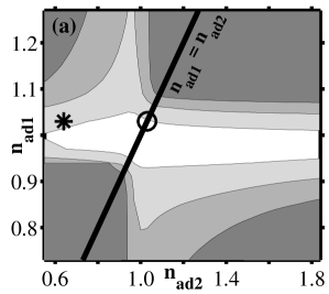
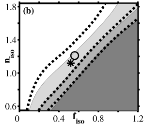
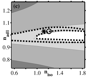
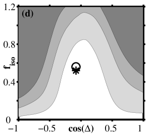
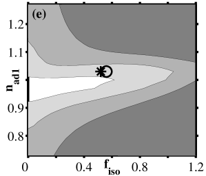
Figure 1(c) should be compared with the results obtained for an uncorrelated mixture of adiabatic and isocurvature fluctuations in Enqvist:2000hp . Although qualitatively similar, the $1\sigma$ and $2\sigma$ regions of uncorrelated models are much smaller than in Enqvist:2000hp due to improved accuracy of the data. We also notice that allowing for correlated models significantly enlarges the $2\sigma$ allowed region in the parameter space.

Since the correlation amplitude is $f_{\rm iso}\cos\Delta$, it is natural that for a high isocurvature fraction $f_{\rm iso}$ the data prefer smaller $|\cos\Delta|$, which is evident in Fig. 1(d). Comparing one-dimensional marginalized likelihoods for $n_{\rm ad1}$ in the pure adiabatic case and in the correlated models we find that allowing for a correlation does not affect much the usual adiabatic spectrum, which is nearly scale free: $n_{\rm ad1}=0.97\pm 0.06$ (pure adiabatic), $n_{\rm ad1}=0.98\pm 0.07$ (correlated models). However, Fig. 1(e) shows that increasing the isocurvature fraction leads to slightly stricter bounds for $n_{\rm ad1}$.

Figure 2: An example of a model that is within $2\sigma$ from our best-fit model. In the temperature power spectrum (a) the vertical axis is $l(l+1)C_{l}/2\pi$ and in the TE cross-correlation spectrum (b) the vertical axis is $(l+1)C_{l}/2\pi$!

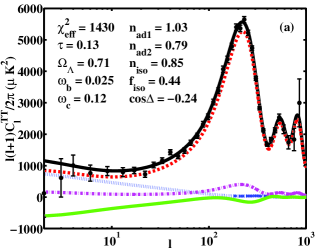
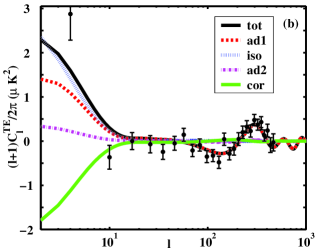
To demonstrate the role of the different components of the spectrum, we plot an angular power spectrum of a $2\sigma$ allowed model in Fig. 2. In this particular model, a high 64% contribution of isocurvature to the total $C_{l}^{TT}$ at the quadrupole (l=2) is allowed since the negative correlation mostly cancels the excess power. In the TE power spectrum there is 103% of isocurvature at the quadrupole. In $C_{l}^{TE}$ the cancellation between the correlation and isocurvature is not exact at the quadrupole, so that the isocurvature adds some power there compared to pure adiabatic models. The wmap measured a very high quadrupole in TE spectrum, which was regarded as a hint for an unexpectedly large optical depth due to reionization $\tau=0.17\pm 0.04$ WMAP1 . In positively correlated models one would easily get a high TE quadrupole even with much smaller $\tau$. However, positive correlation is not favored by TT spectrum where the measured quadrupole is very low. In any case, in most models allowing for correlation adds some power at TE quadrupole, which explains our observation that correlated models seem to favor slightly smaller $\tau$ than pure adiabatic models. On the other hand, strong negative correlation along with quite a large $\tau$ might give a reasonable fit to both the low TT and the high TE quadrupole.

The isocurvature modes introduce also another degeneracy for main cosmological parameters. Namely, allowing for general initial conditions prevents one from determining $\omega_{b}$ from the CMB Trotta:2001yw . Nearly any value for $\omega_{b}$ is allowed, since it is determined by the relative heights of the acoustic peaks, which are also affected by even a small isocurvature or correlation contribution. In our case the degeneracy is even more severe than in Trotta:2001yw , since we allow for independently varying spectral indices. The big bang nucleosynthesis calculations are valuable to determine $\omega_{b}$.

References

- (1) E. Pierpaoli, J. Garcia-Bellido and S. Borgani, JHEP 9910, 015 (1999) [hep-ph/9909420].
- (2) K. Enqvist, H. Kurki-Suonio and J. Valiviita, Phys. Rev. D 62, 103003 (2000) [astro-ph/0006429].
- (3) K. Enqvist and H. Kurki-Suonio, Phys. Rev. D 61, 043002 (2000) [astro-ph/9907221].
- (4) D. Langlois, Phys. Rev. D 59, 123512 (1999); M. Bucher, K. Moodley and N. Turok, Phys. Rev. D 66, 023528 (2002) [astro-ph/0007360]; D. Langlois and A. Riazuelo, Phys. Rev. D 62, 043504 (2000) [astro-ph/9912497].
- (5) J. Garcia-Bellido and D. Wands, Phys. Rev. D 52, 6739 (1995) [gr-qc/9506050]; J. Garcia-Bellido and D. Wands, Phys. Rev. D 53, 5437 (1996) [astro-ph/9511029]; F. Finelli and R. H. Brandenberger, Phys. Rev. D 62, 083502 (2000) [hep-ph/0003172].
- (6) C. Gordon, D. Wands, B. A. Bassett and R. Maartens, Phys. Rev. D 63, 023506 (2001) [astro-ph/0009131].
- (7) L. Amendola, C. Gordon, D. Wands and M. Sasaki, Phys. Rev. Lett. 88, 211302 (2002) [astro-ph/0107089].
- (8) C. Gordon, astro-ph/0112523.
- (9) K. Enqvist, H. Kurki-Suonio and J. Valiviita, Phys. Rev. D 65, 043002 (2002) [astro-ph/0108422].
- (10) C. B. Netterfield et al., Astrophys. J. 571, 604 (2002) [astro-ph/0104460]; A. T. Lee et al., Astrophys. J. 561, L1 (2001) [astro-ph/0104459].
- (11) R. Trotta, A. Riazuelo and R. Durrer, Phys. Rev. Lett. 87, 231301 (2001) [astro-ph/0104017].
- (12) C. L. Bennett et al., astro-ph/0302207.
- (13) A. Kogut et al., astro-ph/0302213.
- (14) H. V. Peiris et al., astro-ph/0302225.
- (15) V. Muhonen and J. Valiviita, in preparation.
- (16) N. Bartolo, S. Matarrese and A. Riotto, Phys. Rev. D 64, 123504 (2001) [astro-ph/0107502].
- (17) S. Tsujikawa, D. Parkinson and B. A. Bassett, astro-ph/0210322.
- (18) “Code for Anisotropies in the Microwave Background” http://camb.info/; A. Lewis and A. Challinor, Phys. Rev. D 66, 023531 (2002) [astro-ph/0203507]; A. Lewis, A. Challinor and A. Lasenby, Astrophys. J. 538, 473 (2000) [astro-ph/9911177].
- (19) N. Christensen, R. Meyer, L. Knox and B. Luey, astro-ph/0103134; A. Lewis and S. Bridle, Phys. Rev. D 66, 103511 (2002) [astro-ph/0205436].
- (20) D. N. Spergel et al., astro-ph/0302209.
- (21) L. Verde et al., astro-ph/0302218.
- (22) G. Hinshaw et al., astro-ph/0302217.