Non-Gaussianity of the derived maps from the first-year WMAP data

Abstract

We present non-Gaussianity testing on recently-released derived maps from the first-year WMAP data by Tegmark, de Oliveria-Costa and Hamilton. Our test is based on a phase mapping technique which has the advantage of testing non-Gaussianity at separate multipole bands. We show that their foreground-cleaned map is against the random-phase hypothesis at all 4 multipole bands centered around $\ell=150$, 290, 400 and 500. Their Wiener-filtered map, on the other hand, is Gaussian for $\ell<250$, and marginally Gaussian for $224<\ell<350$. However, we see the evidence of non-Gaussianity for $\ell>350$ as we detect certain degrees of phase coupling, hence against the random-phase hypothesis. Our phase mapping technique is particularly useful for testing the accuracy of component separation methods.

1 Introduction

With the first-year data release of the Wilkinson Microwave Anisotropy Probe (WMAP ), it has been proclaimed that we have entered the era of “precision cosmology”. The temperature fluctuations of the cosmic microwave background (CMB) radiation are believed to be the imprint of primordial density fluctuations in the early Universe which give rise to the large-scale structures we see today. Hence the data enable us to test the statistical character of the primordial fluctuations, making subsequent inferences on the topology and content of the Universe.

Although the WMAP team (Komatsu et al., 2003) claims that the signal is Gaussian with 95% confidence, the internal linear combination map released by the WMAP team is not up for CMB studies due to “complex noise properties” . Another group led by M. Tegmark has performed an independent foreground cleaning from the first-year WMAP data and made public their whole-sky CMB maps. Their foreground-cleaned map (hereafter FCM) and the Wiener-filtered map (WFM) are available online (Tegmark, 2003).

The FCM by the authors’ definition is such that the foreground contamination is removed as much as possible. As foregrounds are rather non-Gaussian, any residual after cleaning would manifest itself in the phase configuration. In this Letter we display the phases of the FCM and the WFM with color coding and implement our phase-mapping technique to test quantitatively the Gaussianity of both maps, based on the random-phase hypothesis of homogeneous and isotropic Gaussian random fields. Our phase mapping technique can play a crucial role as a qualitative criterion for component separation similar to the field of image reconstruction.

2 Gaussian Random Fields and the Random Phase Hypothesis

The statistical characterization of temperature fluctuation of CMB radiation on a sphere can be expressed as a sum over spherical harmonics:

$$\Delta T(\theta,\varphi)=\sum_{\ell=0}^{\infty}\sum_{m=-\ell}^{\ell}a_{\ell m}Y_{\ell m}(\theta,\varphi),$$ (1)

where $a_{\ell m}=|a_{\ell m}|\exp(i\phi_{\ell m})$. Homogeneous and isotropic Gaussian random fields (GRFs), as a result of the simplest inflation paradigm, possess Fourier modes whose real and imaginary parts are independently distributed. In other words, they have phases $\phi_{\ell m}$ that are independently distributed and uniformly random on the interval $[0,2\pi]$ (BBKS, 1986; Bond & Efstathiou, 1987). Thus the spatial variations should constitute a statistically homogeneous and isotropic GRF (BBKS, 1986) whose statistical properties are completely specified by its angular power spectrum $C_{\ell}$,

$$\langle a_{\ell m}a^{*}_{\ell^{{}^{\prime}}m^{{}^{\prime}}}\rangle=C_{\ell}\;\delta_{\ell\ell^{{}^{\prime}}}\delta_{mm^{{}^{\prime}}}.$$ (2)

The strict definition of a homogeneous and isotropic GRF requires that the amplitudes are Rayleigh distributed and the phases are random (Watts & Coles, 2003). At the same time, the Central Limit Theorem guarantees that a superposition of a large number of Fourier modes with random phases will be Gaussian. Therefore the random-phase hypothesis on its own serves as a definition of Gaussianity (BBKS, 1986).

3 Color-coded phase map of the derived WMAP maps

Tegmark, de Oliveira-Costa & Hamilton (2003) (TDH03) perform an independent foreground analysis from the WMAP data and provide a FCM and WFM. We first use a visual display of phases by colors to show phase associations (Coles & Chiang, 2000). In color image display devices, each pixel represents the intensity and color at that position in the image. Two color schemes are usually used for the quantitative specification of color, namely the Red-Green-Blue (RGB) and Hue-Saturation-Brightness (HSB) color schemes. Hue is the term used to distinguish between different basic colors (blue, yellow, red and so on). Saturation refers to the purity of the color, defined by how much white is mixed with it. Brightness indicates the overall intensity of the pixel on a grey scale. The HSB color model is particularly useful because of the properties of the ‘hue’ parameter, which is defined as a circular variable. Therefore we are mapping phases from 0 to $2\pi$ to the hue circle.

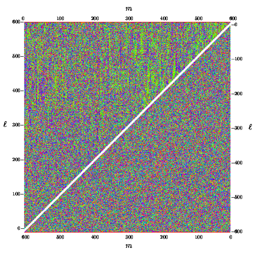
We have used the Healpix package to produce $a_{\ell m}$. In Fig. 3 we show the color-coded phase gradient $D_{\ell}\equiv\phi_{\ell+1,m}-\phi_{\ell,m}$ for the FCM and WFM. The vertical axis is the multipole $\ell$ up to $\ell=600$ and the horizontal the $m$ axis where $m\leq\ell$. Due to the relation $a_{\ell m}=a^{*}_{\ell,-m}$, only modes from non-negative $m$ are shown. Although the phase gradient (from neighboring modes) is the most primitive way of qualitatively checking phase correlations, the apparent presence of stripes shown in the FCM indicates strong coupling between modes of neighboring $\ell$ of the same $m$.

Figure 1: Color-coded phase gradient $D_{\ell}$ for the FCM (upper left triangle) and the WFM (bottom right). The vertical axis is the $\ell$ up to $\ell=600$ and horizontal the $m$ axis. Due to the relation $a_{\ell,m}=a^{*}_{\ell,-m}$, we only show modes from non-negative $m$. Although the phase gradient (from neighboring modes) is the most primitive, the stripes shown from the FCM indicate strong phase correlation between modes of neighboring $\ell$ of the same $m$.

4 Phase mapping and the mean chi-square statistic of the derived maps

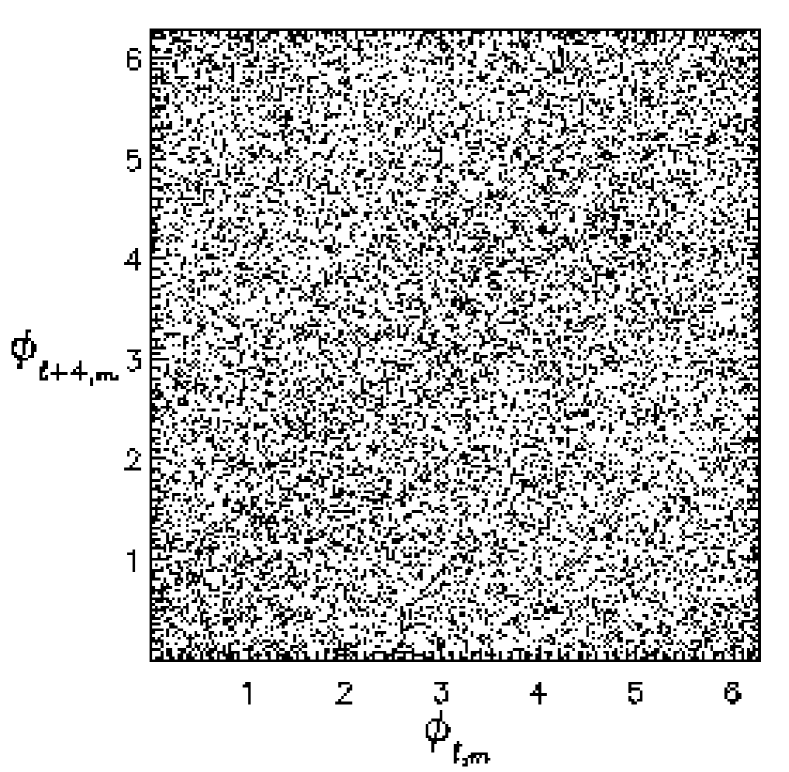
To test the Gaussianity of the FCM and the WFM based on the random-phase hypothesis, we apply a phase mapping technique (Chiang, Coles & Naselsky, 2002; Chiang, Naselsky & Coles, 2002) to quantify the degree of ‘randomness’ of the phases (i.e. Gaussian). The return map of phases is a bounded square in which all phase pairs of fixed separation $(\Delta m,\Delta\ell)$ are mapped as points (see Fig. 4). For example, one single return map for phase pairs with separation $(\Delta m,\Delta\ell)=(0,1)$ contains points with $(x,y)$ coordinate $(\phi_{\ell,m},\phi_{\ell+1,m})$, i.e. all phase pairs from modes that are separated by $\Delta\ell=1$. If the phases are random, we expect to have an ensemble of return maps of all possible separations, each of which should be a scatter plot. As such we are testing the ‘randomness’ on the most strict terms. After mapping phase pairs on to a return map, we can apply a mean $\chi^{2}$ statistic on the return map, which is defined as

$$\overline{\chi^{2}}=\frac{1}{M}\sum_{i,j}\frac{\big{[}p(i,j)-\overline{p}\big{]}^{2}}{\overline{p}},$$ (3)

where $M$ is the number of pixels on the return map, $\overline{p}$ is the mean value for each pixel on the discretized return map. Chiang, Naselsky & Coles (2002) have shown that for a homogeneous and isotropic GRF, return mapping of phases results in an ensemble of return maps, each with a Poisson distribution. The expectation value of the $\overline{\chi^{2}}$ from such ensembles of Poisson-distributed maps is

$$\langle\overline{\chi^{2}}\rangle_{\rm P}=\frac{1}{4\pi R^{2}},$$ (4)

where $R$ is the scale of smoothing from a 2D Gaussian convolution in order to probe the spatial structure. The $\overline{\chi^{2}}_{\rm P}$ will have a statistical spreading around $\langle\overline{\chi^{2}}\rangle_{\rm P}$ with a dispersion $\Sigma_{\rm P}$ where

$$\Sigma_{\rm P}^{2}=\frac{1}{\pi^{3}R^{2}(M/2)}.$$ (5)

Figure 2: An example of a return map for $(\Delta m,\Delta\ell)=(0,4)$ of phases $\phi_{\ell,m}$ of the FCM where $41<\ell<250$. The $\overline{\chi^{2}}$ of this return map is 0.0332 when it is discretized into $128^{2}$ pixels with smoothing scale $R=2$.

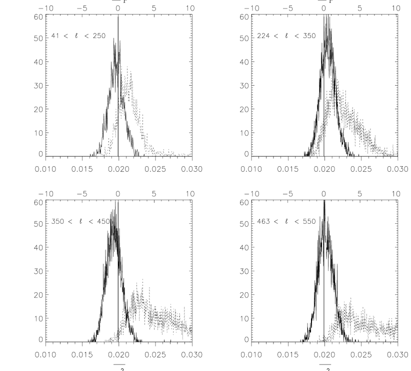
Figure 4 shows the histograms of the $\overline{\chi^{2}}$ statistics from the ensemble of the return maps of the FCM and the WFM for 4 multipole bands. One of the advantages of phase mapping technique is that we are able to check Gaussianity in different multipole bands, in particular those corresponding to foreground contamination and noise. Here we present the $\overline{\chi^{2}}$ statistic at 4 bands centered around $\ell\simeq 150$, 290, 400 and 500: $41<\ell<250$ (roughly the first Doppler peak), $224<\ell<350$, $350<\ell<450$ and $463<\ell<550$. The solid dark and dotted gray curves are the WFM and FCM, respectively. In each panel the vertical line denotes the expectation value $\langle\overline{\chi^{2}}\rangle_{\rm P}=(4\pi R^{2})^{-1}$. The curves from the FCM are obviously skewed, and hence are manifestations of phase correlations (i.e. non-Gaussian).

Figure 3: The histograms of $\overline{\chi^{2}}$ statistic for the FCM (the dotted gray curves) and the WFM (the solid dark curves) at different multipole ranges $\ell$. One of the advantages of the phase mapping technique is that it enables us to check non-Gaussianity for different multipole ranges. The upper horizontal axis is annotated in terms of the theoretical dispersion $\Sigma_{\rm P}$ of GRFs with origin set at the expectation value $\langle\overline{\chi^{2}}\rangle_{\rm P}=(4\pi R^{2})^{-1}$ (vertical line in each panel). The smoothing scale on the $M=128^{2}$ discretized return map is $R=2$.

In Fig. 4 we display the gross behavior of the distribution curves in terms of the arithmetic mean $\langle\overline{\chi^{2}}\rangle$ and the dispersion $\Sigma$ from the mean chi-square statistic. The top panel is from the FCM and the bottom WFM. The contours mark 68% (solid curve) and 95% (dotted curve) CL regions from 2000 realizations of GRFs. The symbols corresponds to 4 multipole bands centered at $\ell\simeq 150$, 290, 400 and 500. Note that the contour region in the bottom panel corresponds to a small section in the top panel. The phases of the 4 multipole bands from the FCM are all strongly correlated, so they are far away from the 95% CL region. The WFM, however, shows that phases below the first Doppler peak are random, with the other 3 multipole bands around the edge of 68% CL region.

We see evidence of non-Gaussianity, however, in the WFM of the following two bands centered $\ell\simeq 400$ and 500. In the lower two panels of Fig. 4 there are points appearing at the tails above $6\Sigma_{\rm P}$. On the other hand, among the 2000 realizations we simulate for GRFs, no mapping of phases reaches $\overline{\chi^{2}}$ value over $6\Sigma_{\rm P}$, setting the probability below 0.05% for a GRF to have such mapping. Phase mapping from the separation $(\Delta m,\Delta\ell)=(0,2)$ produces $\overline{\chi^{2}}$ value at $7.3\Sigma_{\rm P}$ for the multipole band centered $\ell\simeq 400$, also at $6.5\Sigma_{\rm P}$ at $(\Delta m,\Delta\ell)=(1,2)$. For the band $\ell\simeq 500$, $7.6\Sigma_{\rm P}$ appears at $(\Delta m,\Delta\ell)=(2,2)$. These phase couplings are clear signs against the random-phase hypothesis, therefore a manifestation of non-Gaussianity.

Figure 4: The mean chi-square statistic from the FCM (top) and WFM (bottom) against 2000 realizations of GRFs, which is displayed in terms of the arithmetic mean $\langle\overline{\chi^{2}}\rangle$ and the dispersion $\Sigma$ of their distribution curves. The contours mark 68% (solid curve) and 95% (dotted curve) CL regions from 2000 realizations of GRFs. Although 68% and 95% denotes 1 and 2-$\sigma$ deviation in Gaussian statistics, the distribution is not Gaussian but rather chi-square. The cross ($\times$), triangle ($\bigtriangleup$), square ($\Box$) and star ($\ast$) symbols denote $\overline{\chi^{2}}$ statistic from multipole ranges centered $\ell\simeq 150$, 290, 400 and 500, respectively. Note that the contour region in the bottom panel corresponds to a small section in the top panel.

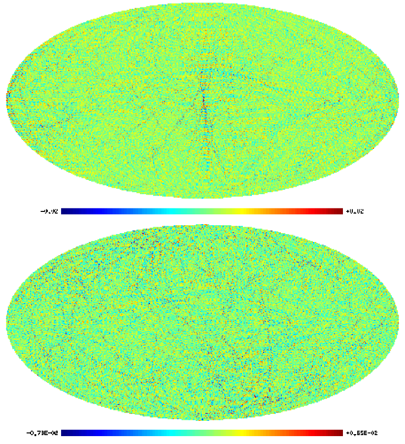
We plot in Fig. 4 the CMB temperature map from only two multipoles $\ell=350$ and 352 (of all $m$’s) of the FCM and WFM. The choice of these specific multipoles of $\Delta\ell=2$ from our previous calculation is to demonstrate non-Gaussian signals the correlated phases will produce in the map. The structures at $\varphi\simeq 0$ and $\pi$ in the FCM, the residual signal after foreground cleaning, disappear after Wiener filtering.

Figure 5: The CMB temperature from two multipoles $\ell=350$ plus 352 of the FCM (top) and the WFM (bottom). These two multipole modes are chosen because of the pronounced coupling between modes $\Delta\ell=2$ of all $m$’s. The structures at $\varphi\simeq 0$ and $\pi$ shown in the FCM disappear after Wiener filtering, from which it is marginally Gaussian at these two multipoles.

5 Discussions

In this Letter we have tested non-Gaussianity of two maps: the Foreground-cleaned map and the Wiener-filtered map, which are processed by TDH03 from the WMAP data. Based on the random-phase hypothesis, we use a phase mapping technique to yield a statistic that has detected considerable non-Gaussian signals for both maps at most multipole bands. Our phase mapping technique is particularly useful in separating non-Gaussian contributions from different sources when various contaminations are present at different $\ell$ ranges. A multipole band which is considerably non-Gaussian could have an insignificant non-Gaussian contribution in the whole map and still produce an over-all Gaussian realization within a certain confidence level. As the uncertainties in foreground cleaning propagate through the data-processing pipelines to the accuracy of the angular power spectrum, it is therefore necessary to have effective methods in component separation. We believe that our phase mapping technique is a useful criterion to be incorporated into such methods. Our statistic based on phase mapping also holds great advantage when it comes to the issue of creating many whole-sky Gaussian realizations for Gaussian statistics. As our null hypothesis is that phases are random, we only need to put random phases (with Gaussian instrumental noise being automatically included) for each harmonic mode, which is easily done without any limit on the highest harmonic number $\ell$ from any pixelization scheme. It is worth mentioning that the upcoming Planck mission will have higher sensitivity and resolution, hence every step of data processing will be crucial in reaching such precision.

References

- BBKS (1986) Bardeen J. M., Bond J. R., Kaiser N., & Szalay A. S. 1986, ApJ, 304, 15
- Bond & Efstathiou (1987) Bond, J. R., & Efstathiou, G. 1987, MNRAS, 226, 655
- Bennett et al. (2003a) Bennett, C. L. et al., 2003, ApJ, 583, 1
- Bennett et al. (2003b) Bennett, C. L. et al., 2003, ApJ submitted (astro-ph/0203208)
- Chiang, Coles & Naselsky (2002) Chiang, L.-Y., Coles, P., & Naselsky, P. D. 2002, MNRAS, 337, 488
- Chiang, Naselsky & Coles (2002) Chiang, L.-Y., Naselsky, P. D., & Coles, P. 2002 (astro-ph/0208235)
- Coles & Chiang (2000) Coles, P., & Chiang, L.-Y. 2000, Nature, 406, 376
- Górski, Hivon & Wandelt (1999) Górski, K. M., Hivon, E., & Wandelt, B. D. 1999, Proceedings of the MPA/ESO Cosmology Conference “Evolution of Large-Scale Structure”, eds. A. J. Banday, R. S. Sheth and L. Da Costa, PrintPartners Ipskamp, NL
- Komatsu et al. (2003) Komatsu E. et al. 2003, ApJ submitted (astro-ph/0203223)
- Tegmark (2003) Tegmark, M. 2003, http://www.hep.upenn.edu/~max/wmap.html
- Tegmark, de Oliveira-Costa & Hamilton (2003) Tegmark, M., de Oliveira-Costa, A., & Hamilton, A. 2003 Phys. Rev. Dsubmitted (astro-ph/03022496)
- Watts & Coles (2003) Watts, P. I. R., & Coles, P. 2003, MNRAS, 338, 806