Where is the second planet in the HD 160691 planetary system?

Abstract

The set of radial velocity measurements of the HD 160691 has been recently published by Jones et al. (2002b). It reveals a linear trend that indicates a presence of the second planet in this system. The preliminary double-Keplerian orbital fit to the observations, announced by the discovery team, describes a highly unstable, self-disrupting configuration. Because the observational window of the HD 160691 system is narrow, the orbital parameters of the hypothetical second companion are unconstrained. In this paper we try to find out whether a second giant planet can exist up to the distance of Jupiter and search for the dynamical constraints on its orbital parameters. Our analysis employs a combination of fitting algorithms and simultaneous examination of the dynamical stability of the obtained orbital fits. It reveals that if the semi-major axis of the second planet is smaller than $\simeq 5.2$ AU, the observations are consistent with quasi-periodic, regular motions of the system confined to the islands of various low-order mean motion resonances, e.g., 3:1, 7:2, 4:1, 5:1, or to their vicinity. In such cases the second planet has smaller eccentricity $\simeq 0.2-0.5$ than estimated in the previous works. We show that the currently available Doppler data rather preclude the 2:1 mean motion resonance expected by some authors to be present in the HD 160691 system. We also demonstrate that the MEGNO-penalty method (MEGNO is an acronym for the Mean Exponential Growth factor of Nearby Orbits), developed in this paper, which is a combination of the genetic minimization algorithm and the MEGNO stability analysis, can be efficiently used for predicting stable planetary configurations when only a limited number of observations is given or the data do not provide tight constraints on the orbital elements.

1 Introduction

Recently, Jones et al. (2002b) have published the radial velocity (RV) observations of a metal-reach solar-type star HD 160691 . These data, consisting of 38 RV measurements and having the formal uncertainties in the range $2.3$–$6.3$ $\mbox{ms}^{-1}$, upgrade the RV data published in Butler et al. (2001) and in the preprint (Jones et al., 2002a), which quotes a smaller number, 33, of the RV measurements than in its published version. As it will become clear later, both references are relevant to our discussion. These new data make it possible to refine a preliminary initial parameters of the HD 160691 system given in Butler et al. (2001). The new data confirm the Keplerian elements of the previously detected planet and reveal a linear trend indicating that a second planet in the HD 160691 system is possible. In the preprint (Jones et al., 2002a), the approximate orbital elements of the second companion indicate a proximity of the HD 160691 system to the 2:1 mean motion resonance (MMR). Such possibility is puzzling because the HD 160691 system would be the third instance of this resonance (in addition to systems around Gliese 876 and HD 82943) among only a dozen of multi-planetary exosystems known to date. However, the initial parameters reproduced in Table 1 as the fit J2, and considered as osculating Keplerian elements, describe orbits that cross each other. This leads to a rapid disintegration of the system. The updated orbital fit given in Jones et al. (2002b) is highly unstable, either, and it rather precludes the inquiring case of the 2:1 MMR (Table 1, fit J2a). However, the authors stress that in both cases the initial elements of the hypothetical second planet are not constrained and very uncertain.

In this work we analyze the published RV data of the HD 160691 system in a more general manner — beyond a formal fit of the Keplerian orbital elements. Although the RV data do not provide tight constrains on the orbital elements of the second planet, these elements are confined by the dynamics, especially in a case when the second companion is not very far from the inner planet. This relevant information is entirely omitted in the Keplerian fit. Applying the Copernican principle, it is not likely to observe planetary systems during moments of their extraordinary orbital evolution (Murray & Holman, 2001). But a disruption of a planetary system is an unusual event and we can argue that if by a formal fit, we find the initial conditions that lead to such a phenomenon then this fit is unlikely either. In this sense, the system dynamics becomes an observable that should be taken into account together with the RV observations while looking for the possible orbital parameters of a planetary system. This way of reasoning has already been applied by skipping orbital fits that lead to highly unstable systems (see, for instance Stepinski et al., 2000; Laughlin & Chambers, 2001; Rivera & Lissauer, 2001; Goździewski & Maciejewski, 2001). It has also inspired us to ask whether the current, limited RV data set of the HD 160691 system merged with the dynamical analysis of the obtained best fit orbital parameters can provide enough information to estimate meaningful limits on the orbital parameters of the hypothetical second planet. In this paper we also describe a method that can be useful in resolving this generic problem not only for the HD 160691 system, chosen as an excellent candidate for such analysis, but in all other cases when the RV observations do not supply sufficient constraints on the orbital parameters of planetary companions.

2 Overall dynamical characteristic of the HD 160691 system

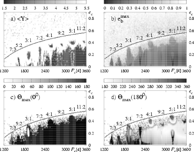
The analysis of the HD 160691 system in this paper relies on the radial velocity observations presented in the preprint by Jones et al. (2002a) and their recently published paper (Jones et al., 2002b). Even simple considerations lead to the conclusion that the approximate fits published in these papers are generically unstable for large eccentricities of the putative planet c. If we assume that $1.5~{}\mbox{AU}<a_{{\mbox{\scriptsize c}}}<5.2$ AU, then in a stable system $e_{{\mbox{\scriptsize c}}}$ cannot be larger than $\simeq 0.6$—otherwise the orbits cross each other and a collision occurs. For a reference see Figure 4, where we show approximate planetary collision line, determined through $a_{{\mbox{\scriptsize b}}}(1+e_{{\mbox{\scriptsize b}}})=a_{{\mbox{\scriptsize c}}}(1-e_{{\mbox{\scriptsize c}}})$, and calculated for $e_{{\mbox{\scriptsize b}}}=0.31$ and $a_{{\mbox{\scriptsize b}}}=1.49$ AU. These values are justified by the fits of Jones et al. (2002a, b) and our solutions. The orbital parameters of the inner planet are well constrained by the RV data. If $e_{{\mbox{\scriptsize c}}}$ is really large, larger than the critical collisional value, the planets can avoid collisions only when a dynamical mechanism prevents them from an encounter. It is well known, that this can be provided by orbital resonances. These resonances are present in many multi-planetary exosysystems (see Table 8 in Fischer et al., 2003). Thus, assuming that the hypothetical giant planet’s orbit is somewhere up to the Jupiter distance, $\simeq 5.2$ AU from the star, the mutual interactions between the companions are substantial and it is reasonable to expect the existence of an orbital resonance in the HD 160691 system. For the hypothetical 2:1 MMR, it should be accompanied by the secular apsidal resonance (SAR), $\varpi_{{\mbox{\scriptsize b}}}\simeq\varpi_{{\mbox{\scriptsize c}}}$. This has been studied in detail in many recent papers about Gliese 876 (e.g., Laughlin & Chambers, 2001; Rivera & Lissauer, 2001; Lee & Peale, 2002; Goździewski et al., 2002; Ji et al., 2002; Hadjidemetriou, 2002) and HD 82943 Goździewski & Maciejewski (2001); Hadjidemetriou (2002); Jiang-Hui et al. (2002). These systems are striking examples of the protective role of the 2:1 MMR accompanied by the SAR. These resonances, acting together, permit for stable planetary configurations even for extremely high eccentricities, $\simeq 0.95-0.98$ Goździewski et al. (2002). It could help us explain a very large eccentricity of the second planet and maintain the system stability in spite of a generic obscure to a stable orbital evolution which comes from the possibility of close encounters. In the light of unconstrained orbital elements of the outer companion, the question whether a stable 2:1 MMR is permissible in the HD 160691 system is an attractive and challenging subject of study.

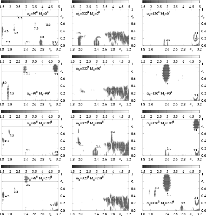
To get an overview of the possible dynamical states of the system we calculated a number of the MEGNO stability maps in the ($a_{{\mbox{\scriptsize c}}},e_{{\mbox{\scriptsize c}}}$)-plane, centered on the nominal position of this resonance, about $2.4$ AU. We assumed that the orbital elements of the inner planet are fixed at the J2 fit (see Table 1). These data have been considered as the osculating, astrocentric elements at the epoch of the periastron passage of the outer planet. As we already mentioned, in both the fits J2 and J2a, as well as in our solutions (they will be described later), the elements of the inner companion are very similar and we considered them well constrained by the observations. We assumed that the system is coplanar and edge-on. This assumption reduces greatly the number of possible orbital configurations but the ($a_{{\mbox{\scriptsize c}}},e_{{\mbox{\scriptsize c}}}$)-plane is dynamically representative for the system dynamics, in the sense that it crosses all resonances Robutel & Laskar (2001). Moreover, the widths of MMRs depend on the phases of companions and for this reason we varied, in subsequent maps, the initial longitude of periastron and the mean anomaly of the outer planet. The results of the experiment are illustrated in Figure 1. In the test, $\omega_{{\mbox{\scriptsize c}}}=99^{\circ}$ is equal to its formal fit value and corresponds to the first column of the MEGNO-maps which are calculated for the initial mean anomaly $M_{{\mbox{\scriptsize c}}}=0^{\circ}$, $90^{\circ}$, $180^{\circ}$ and $270^{\circ}$, respectively, i.e., for different initial phases of the outer planet. Simultaneously, the initial orbital phase of the inner planet has been fixed at $\omega_{{\mbox{\scriptsize b}}}=320^{\circ}$ and $M_{{\mbox{\scriptsize b}}}\simeq 10^{\circ}$. The middle and the right columns in Figure 1 are for $\omega_{{\mbox{\scriptsize c}}}\simeq 320^{\circ}$ and $\omega_{{\mbox{\scriptsize c}}}\simeq 120^{\circ}$, respectively. These values have been selected in such a way that the apsidal lines are intially aligned (Figure 1, middle column) or antialigned (Figure 1, right column).

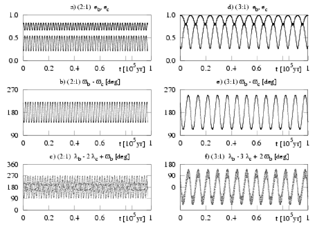
The scans corresponding to the nominal initial condition (IC, the first column in Figure 1), reveal a number of very narrow zones of stable motions. They are identified with the low-order MMRs, e.g., 4:3, 7:5, 3:2, 5:3, 2:1, 7:3, 5:2, 8:3 and 3:1. In the scans for $M_{{\mbox{\scriptsize c}}}=90^{\circ}$ and $M_{{\mbox{\scriptsize c}}}=270^{\circ}$, we discovered extended islands of stable 2:1 MMR for large $e_{{\mbox{\scriptsize c}}}$. As we expected, this resonance is accompanied by the SAR, with apsidal lines librating about $180^{\circ}$. This is illustrated in Fig 2a,b,c. In the MEGNO-scans, we also found a stable island of the 3:1 MMR, which is present for extremely large eccentricities of the outer planet, up to 0.98! The evolution of the astrocentric orbital elements is illustrated in Figure 2d,e,f. Outside the MMRs zones, the planetary configurations are very unstable and typically self-disrupt rapidly (on timescales of a few years).

As we already mentioned, the IC quoted in Jones et al. (2002a) is very close to a stable island of the 2:1 MMR. In order to lock the dynamics in this resonance, a change of the orbital phase of the outer planet from (the formal value) $M_{{\mbox{\scriptsize c}}}\simeq 0^{\circ}$ to $M_{{\mbox{\scriptsize c}}}\simeq 90^{\circ}$ is required. One would think that such a change may be permissible since the orbital parameters are weakly constrained by the data, but in fact, the synthetic RV curve is strongly affected by a modification of the relative phases of the planets (for an example see section 5). Actually, the scans shown in Figure 1, suggest that by changing the weakly constrained or unconstrained parameters of the outer planet, we can also obtain many other, stable resonance configurations. However, similarly to the previous case, it does not necessarily mean that these configurations would produce Doppler signals which are consistent with the RV observations. Because the linear trend present in the RV data is only at best a ”fingerprint” of the second companion, any additional observations significantly alter the orbital fit. For these reasons a detailed, global analysis of the stability of a few orbital configurations of the HD 160691 system, defined by the very uncertain fits, is a hopeless task, if we aspire to investigate systems that are at least similar to the observed one. In the next section we show that in fact the linear trend present in the data permits for a continuum of equally good orbital fits. This has been already pointed out by Jones et al. (2002b).

3 Global 2-Keplerian fit to the RV data

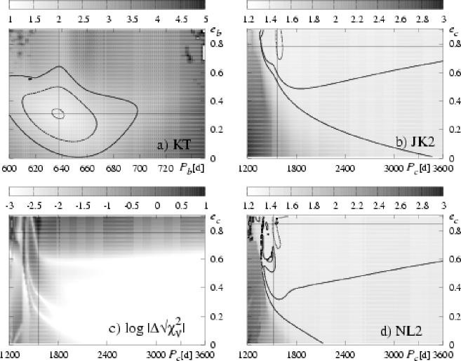
Following the arguments given in in the introduction, we try to reduce the number of possible orbital configurations of the HD 160691 system by analyzing ${(\chi^{2}_{\nu})^{1/2}}$-goodness of the fits simultaneously with the dynamical character of the resulting IC. In order to find the best double-Keplerian fit, we were applying the RV models that were subsequently more and more elaborate. At first, we assumed that the data can be approximated by a sum of the one-Keplerian RV signal and a linear trend (the KT model). Note that our model of the Keplerian RV signal differs from the classical version which is really suitable for binary stellar systems (see the Appendix for all details). To perform a global search for the best fit, we computed the function ${(\chi^{2}_{\nu})^{1/2}}(P_{{\mbox{\scriptsize b}}},e_{{\mbox{\scriptsize b}}})$ in the $(P_{{\mbox{\scriptsize b}}},e_{{\mbox{\scriptsize b}}})$-plane, fixing $P_{{\mbox{\scriptsize b}}}$ and $e_{{\mbox{\scriptsize b}}}$ in the ranges $[600-700]$ d and $[0,0.9]$, respectively. The Levenberg-Marquardt (LM) minimization scheme (Press et al., 1992) was used to find the best fit at every point of the $100\times 100$-data grid in this region. We searched for the best fits at every point of the grid by varying the starting phase of the inner planet with the step of $30^{\circ}$. The obtained ${(\chi^{2}_{\nu})^{1/2}}$-map reveals a very well determined minimum of ${(\chi^{2}_{\nu})^{1/2}}$ (see Fig. 3a) corresponding to $P_{{\mbox{\scriptsize b}}}\simeq 638$ d and $e_{{\mbox{\scriptsize b}}}\simeq 0.31$. These parameters coincide very well with the solution given in Jones et al. (2002a) and Jones et al. (2002b). The fit has ${(\chi^{2}_{\nu})^{1/2}}\simeq 1.48$ and rms $\simeq 4.8\mbox{ms}^{-1}$.

Next, we assumed that the linear trend can be explained as the presence of a second companion in the system . Taking the best fit parameters of the KT model as an approximation of the orbital elements of the inner companion, we calculated the function ${(\chi^{2}_{\nu})^{1/2}}(P_{{\mbox{\scriptsize c}}},e_{{\mbox{\scriptsize c}}})$ for the double-Keplerian (JK2) model. At every point of the grid, $P_{{\mbox{\scriptsize c}}}\in[1200,3600]$ d and $e_{{\mbox{\scriptsize c}}}\in[0,0.9]$, the best fit solution was obtained by varying the initial longitudes of periastron and the mean anomalies of each companion with the step of $30^{\circ}$. The result is shown in Fig. 3b. The best fit solution [the JK2 fit, ${(\chi^{2}_{\nu})^{1/2}}\simeq 1.39$ and rms $\simeq 3.9~{}\mbox{ms}^{-1}$, see Table 2] corresponds to $P_{{\mbox{\scriptsize c}}}\simeq 1560$ d and $e_{{\mbox{\scriptsize c}}}\simeq 0.78$. The synthetic RV curve is shown in the left panel of Figure 5. In the entire range of $e_{{\mbox{\scriptsize c}}}$, the fits obtained for $P_{{\mbox{\scriptsize c}}}>1600$ d are of very similar significance because their ${(\chi^{2}_{\nu})^{1/2}}\simeq 1.5$ and the rms is about $4.5~{}\mbox{ms}^{-1}$. This result is not surprising as it reflects the limitation caused by a small number of measurements and a narrow observational window compared to the likely period of the outer companion. However, in the range of small $P_{{\mbox{\scriptsize c}}}$, specifically for the one corresponding to the 2:1 MMR, the double-Keplerian fits are significantly worse.

The global fit, obtained through the $(P_{{\mbox{\scriptsize c}}},e_{{\mbox{\scriptsize c}}})$-scan, has been verified by the minimization method based on the genetic algorithm (GA). The GAs are still not very popular but they have been proved to be very useful for finding good starting points for the precise gradient methods of minimization like e.g. the well known Levenberg-Marquardt scheme. For a very interesting review of the astronomical applications of the GAs see the paper by Charbonneau (1995). To the best of our knowledge this method of minimization was used for analyzing the RV data of $\upsilon$ Andr by Butler et al. (1999) and Stepinski et al. (2000), the Gliese 876 system by Laughlin & Chambers (2001, 2002), and 55 Cnc by Marcy et al. (2002). We also applied it to the HD 12661 system (Goździewski & Maciejewski, 2003). Basically, the genetic scheme makes it possible to find the global minimum of the ${(\chi^{2}_{\nu})^{1/2}}$ function. For computations, we used the publicly available code PIKAIA ver. 1.2 by Paul Charbonneau which allows to limit the search space. This was very useful in our situation, because we could restrict the GA search region to the one analyzed by the JK2 scan method. In many restarts of the GA code, confined to $P_{{\mbox{\scriptsize c}}}\in[1200,3600]$ d, we repeatedly found the best fit which is given in Table 2 as the GA2 solution. It is qualitatively similar to the best JK2 solution. In an additional set of the runs, the range of $P_{{\mbox{\scriptsize c}}}$ has been restricted to [1000,1400] d to cover the hypothetical 2:1 MMR. As it turns out, in this case the best fits have ${(\chi^{2}_{\nu})^{1/2}}\simeq 1.53$, substantially larger than the GA2 solution and correspond to $P_{{\mbox{\scriptsize b}}}\simeq 612$ d, $P_{{\mbox{\scriptsize c}}}\simeq 1400$ d. This is consistent with the results of the JK2 scan search as the best GA in this region were found confined to the area around the limiting $P_{{\mbox{\scriptsize c}}}=1400$ d.

At this point we could say that there is not much more to do unless we try to analyze the dynamical stability of the obtained fits. The results of such an analysis are presented in Figure 4. Panel 4a shows the MEGNO signatures evaluated for every fit in the JK2 scan. For the purpose of this map the Kepler-Jacobi orbital elements are transformed to the osculating, astrocentric elements at the epoch of the first observation. This scan reveals that most of the JK2 fits are chaotic and unstable, including the best fit solution. (The genetic best fit solution GA2 is strongly chaotic too). The border of the dynamical stability, clearly seen in all the panels, is well correlated with the planetary collision line marked with a thick line. The instability, defined through the MEGNO, in the strict sense of regular and chaotic behaviours, is meaningful and leads to macroscopic changes of the orbital elements during a relatively very short integration time. This is illustrated in Figure 4b where we marked the maximal eccentricities of the outer planet attained during the integration timespan equal to at most $\sim 10^{4}$ orbital periods of this planet. The integrations were stopped if one of the eccentricities had become larger than 0.99 or one of the semi-major axes exceeded 10 AU. In these cases, the system has been considered as disrupted. As we could expect, above the planetary collision line, the osculating elements are completely different from their starting values which confirms the dramatic effects of the close encounters or collisions.

Another interesting result, provided by the analysis of the short term dynamics, is shown in Figure 4c,d. It illustrates a detection of the SAR and an estimate of the semi-amplitude of the critical argument $\theta=\varpi_{{\mbox{\scriptsize b}}}-\varpi_{{\mbox{\scriptsize c}}}$. It was derived with the same method which was successfully applied to the HD 12661 system in (Goździewski, 2003). In the MEGNO code, we evaluated the maximal value $\theta_{{\mbox{\scriptsize max}}}$ of $\theta$, after every step of the renormalization of the variational equations (the time step was equal to the orbital period of the outer planet). The maximal value of the critical argument was taken relative to the center of libration $0^{{\rm o}}$ or $180^{\circ}$. To avoid the effects of a possible transition into the apsidal resonance, the determination of $\theta_{{\mbox{\scriptsize max}}}$ was started after the first half of the integration period. Finally, if $\theta_{{\mbox{\scriptsize max}}}<180^{\circ}$, then we treated this value as a semi-amplitude of the apsidal librations. Although the period of integrations is relatively very short, such an approximation of the semi-amplitude already gives much insight into the global dynamics of the system. Note that in the $\theta$-maps we do not mark the systems which collided during the integration time (the white areas above the planetary collision line). Remarkably, both the $\theta$-maps reveal a small, isolated island about $P_{{\mbox{\scriptsize c}}}\simeq 1900$ d related to the 3:1 MMR. In this island the $\theta$ argument librates about $240^{\circ}$. A much more extended stable region emerges for $P_{{\mbox{\scriptsize c}}}>2200$ d. The configurations in this region correspond mostly to the librations of $\theta$ about $180^{\circ}$ (see Figure 4d). An obvious and clear correlation between the MEGNO scan and the MMRs structures is visible in this plot. These structures correspond to a number of the low-order MMRs: e.g., 7:2, 4:1, 5:1.

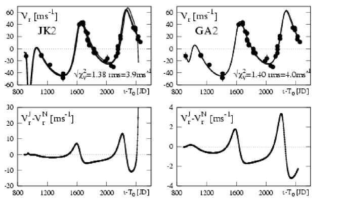
Because the best fit solutions JK2 and GA2 are confined to the $e_{{\mbox{\scriptsize c}}}$ regions where the collisions are very likely, we verified whether the Jacobi-Keplerian fits properly represent the dynamical state of the HD 160691 system. We compared the synthetic RV curve obtained from these models and the RV curve emerging from the full Newtonian mode of the Doppler signal. The top panels in Figure 5 illustrate the synthetic RV curves and the bottom panels are for the appropriate differences between the RV signals. For the GA2 solution the difference reaches about 4 $\mbox{ms}^{-1}$ over the time span of the data set and is comparable to the internal accuracy of the precise RV method. In the case of the JK2 solution, this difference reaches $\simeq 40~{}\mbox{ms}^{-1}$ and is unacceptably large. This comparison demonstrates the obvious need of incorporating the mutual interactions between the companions in the fitted model. This is seen even better in Figure 3c. It illustrates the global effects of neglecting the mutual interactions between the companions in the model. At every point of the JK2-scan (Figure 3b) we computed the value of ${(\chi^{2}_{\nu})^{1/2}}$ emerging from the Keplerian and Newtonian RV signals. Similarly to the previous experiment, the best JK2 fits have been considered as the osculating elements at the epoch of the first observation. We plotted $\log|\Delta{(\chi^{2}_{\nu})^{1/2}}|$, where $\Delta{(\chi^{2}_{\nu})^{1/2}}$ corresponds to a difference of ${(\chi^{2}_{\nu})^{1/2}}$ between the models. This figure shows that the JK2 fits are in fact unacceptable for large $e_{{\mbox{\scriptsize c}}}$. On the other hand, for $P_{{\mbox{\scriptsize c}}}>1800$ d and moderately small $e_{{\mbox{\scriptsize c}}}$, the Keplerian and Newtonian RV curves coincide perfectly. These results confirm once again the remarkable result of Laughlin & Chambers (2001): for strongly interacting systems, the Keplerian fitting has a very limited use.

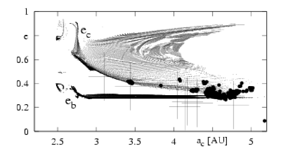
To put this statement into work, we refined the two planet fits using the LM algorithm driven by the full Newtonian model of the RV signal, and taking the Keplerian fits as the starting data to the gradient LM search. Similarly to the previous cases, these fits have been formally transformed to astrocentric osculating Keplerian elements, at the epoch of the first observation. Because in the region of large $e_{{\mbox{\scriptsize c}}}$, the JK2 fits do not describe the system’s state properly, they are unlikely optimal starting points in this area, and it was hard to expect that the LM algorithm will find truly global minimum of ${(\chi^{2}_{\nu})^{1/2}}$. To obtain an approximation of the best Newtonian ${(\chi^{2}_{\nu})^{1/2}}$-scan and to simplify the search, both the masses and $a_{{\mbox{\scriptsize b}}}$ have been fixed at their JK2 values. All other orbital parameters have been fitted by the gradient algorithm. The obtained ${(\chi^{2}_{\nu})^{1/2}}$-map in the $(P_{{\mbox{\scriptsize c}}},e_{{\mbox{\scriptsize c}}})$-plane of the starting orbital elements, is shown in Figure 3d. Clearly, for large $e_{{\mbox{\scriptsize c}}}$ the $N$-body model gives a significant improvement of the ${(\chi^{2}_{\nu})^{1/2}}$ function over the Keplerian model. The best Newtonian fit found in this test is given in Table 2 as the NL2 fit and its synthetic RV curve is shown in the left panel of Figure 6. Unfortunately, this fit is highly unstable too. Finally, we examined the MEGNO signatures of the rest of about 20,000 fits, with about 17,300 cases when ${(\chi^{2}_{\nu})^{1/2}}<1.5$. Only about 260 initial conditions appeared to be dynamically stable, having the MEGNO signature $|\langle Y\rangle-2|<0.05$. About 15,700 IC lead to disruption of the resulting configuration during the global period of time less than 70,000 years. The results are illustrated in Figure 7, which shows the fitted semi-major axis $a_{c}$ of the outer planet versus the fitted eccentricities of the companions. Dots represent the fits with ${(\chi^{2}_{\nu})^{1/2}}<1.5$ and larger, filled circles represent $(a_{{\mbox{\scriptsize c}}},e_{{\mbox{\scriptsize c}}})$ of the quasi-periodic, stable configurations. This figure clearly shows that the stable solutions are grouped in a few distinct islands, the most remarkable of which is the one corresponding to the smallest ${(\chi^{2}_{\nu})^{1/2}}\simeq 1.473$ (about $a_{{\mbox{\scriptsize c}}}\simeq 3.43$ AU). It will be shown in the next section that this island is related to 7:2 MMR. For all of the stable fits, the eccentricity of the outer planet is moderately small compared to the previous estimates. The figure shows also the scale of the uncertainty of parameters form the Newtonian fits: for the statistically similar fits, ${(\chi^{2}_{\nu})^{1/2}}<1.5$, the value of $a_{{\mbox{\scriptsize c}}}$ is spread over $\simeq 2.5~{}$ AU, and $e_{{\mbox{\scriptsize c}}}$ over 0.6. At the same time, $e_{{\mbox{\scriptsize b}}}$ remains well bounded. A sharp limit of possible solutions for about $a_{{\mbox{\scriptsize c}}}>2.5$ AU is clearly visible. All the stable fits have $1.47<{(\chi^{2}_{\nu})^{1/2}}<1.49$, rms $\simeq 4.4~{}\mbox{ms}^{-1}$ and very similar parameters of the inner companion: $e_{{\mbox{\scriptsize b}}}\simeq 0.283$, $\omega_{{\mbox{\scriptsize b}}}\simeq 134^{\circ}$, $M_{{\mbox{\scriptsize b}}}\simeq 344^{\circ}$.

4 Genetic fitting with the MEGNO penalty

Although the best fit solutions obtained with the help of the previous analysis are unstable, there is still no reason to claim that in their neighborhood a stable fit related to a resonance is not possible. We have already analyzed such an instance (Goździewski & Maciejewski, 2001). Following the approach advocated in that paper and in a series of recent works (e.g., Goździewski, 2003; Goździewski & Maciejewski, 2003), we can search for a stable IC by calculating and analyzing the MEGNO stability maps. Moreover, in such a case we have to control how the tested initial condition ”preserves” the ${(\chi^{2}_{\nu})^{1/2}}$ function and the shape of the RV curve. Without such control, it is easy to find a stable initial condition (see the analysis in the section 2) that can lead to a very poor model of the RV observations. Thus, for a desired (stable) solution, we have to calculate its ${(\chi^{2}_{\nu})^{1/2}}$ and decide whether it is acceptable. In this way, we explicitly follow the argumentation given in the introduction, i.e., the system dynamics serves as an additional observable characterizing the planetary system.

In practice such a procedure is very laborious so we have found a way to simplify the search process. For this purpose, we employed the GA minimization. Since the GAs belong to the gradient-free optimization methods, to find the best fit we only have to define the ${(\chi^{2}_{\nu})^{1/2}}$ function. To find the best fits that are simultaneously stable, we proceed as follows. The “fitness” function $f$, required by the GA, which is equivalent to $1/{(\chi^{2}_{\nu})^{1/2}}$, is modified according to the formula $f=1/p[{(\chi^{2}_{\nu})^{1/2}},\langle Y\rangle],$ where $p$ is a “penalty” function. If, for the tested IC, the value of ${(\chi^{2}_{\nu})^{1/2}}$ is less than a prescribed limit ${(\chi^{2}_{\nu})^{1/2}_{{\mbox{\scriptsize max}}}}$, then the MEGNO signature $\langle Y\rangle$ is also computed for this fit. Then, if the tested fit is related to a regular system then $|\langle Y\rangle-2|<\epsilon$ where $\epsilon>0$ is a small value, and $p\equiv{(\chi^{2}_{\nu})^{1/2}}$, i.e., $f$ is unchanged. For a chaotic solution, $|\langle Y\rangle-2|$ grows linearly, and $f$ should diminish substantially. The choice of $p$ is not quite obvious. In our calculations, we tested two forms of the penalty function: $p={(\chi^{2}_{\nu})^{1/2}}+\alpha|\langle Y\rangle-2|,$ and $p={(\chi^{2}_{\nu})^{1/2}}(1+\alpha|\langle Y\rangle-2|),$ where $\alpha>0$. Both give similar convergence and solutions. Otherwise, if ${(\chi^{2}_{\nu})^{1/2}}>{(\chi^{2}_{\nu})^{1/2}_{{\mbox{\scriptsize max}}}}$, then $f$ is left unchanged and the MEGNO test is skipped. This step is very relevant for the numerical efficiency as the calculations of MEGNO are CPU-expensive. The $f$ code depends on three control parameters: ${(\chi^{2}_{\nu})^{1/2}_{{\mbox{\scriptsize max}}}}$, $\epsilon$, and $\alpha$. To gain the desired numerical efficiency, we used the limit $\langle Y\rangle_{{\mbox{\scriptsize max}}}\simeq 5$ for MEGNO, a relatively short integration time (about $10^{3}$ periods of the outer companion), ${(\chi^{2}_{\nu})^{1/2}_{{\mbox{\scriptsize max}}}}=1.6$, $\epsilon\simeq 0.1$ and $\alpha=1$. This integration time is sometimes too short to get a clear MEGNO convergence, but the code quickly eliminates the strongly chaotic systems. This also weakens the requirement of strictly regular, quasiperiodic configurations, and the search does not exclude systems evolving on a border of stability. Obviously, in this approach, the RV model is driven by the full model of the $N$-body dynamics. Because the search is driven by the GA, the MEGNO-penalty algorithm has also a global character.

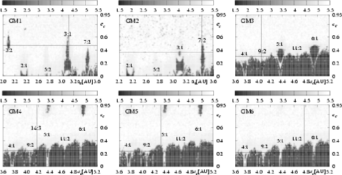
Using the described method in a number of repeated runs of the code, the algorithm converged repeatedly to a few distinct solutions, which are called GM fits from hereafter. Their examples, labeled GM1-GM6, are given in Table 3. At first we limited the search region to $a_{{\mbox{\scriptsize c}}}<3.6$ AU. In this case one could expect solutions corresponding to the lower order resonances, including the 2:1 MMR. Indeed, we found two such different fits: the one corresponding to the 3:1 MMR (GM1, $a_{{\mbox{\scriptsize c}}}$ about 3.1 AU) and the second one related to the 7:2 MMR (GM2, $a_{{\mbox{\scriptsize c}}}$ about 3.44 AU). The GM2 fit appears to be the best stable fit found in the entire search, having ${(\chi^{2}_{\nu})^{1/2}}\simeq 1.47$ and rms $\simeq 4.35~{}\mbox{ms}^{-1}$. At the same time, we did not find any stable solution that would correspond to the 2:1 MMR. In the region $3.6~{}\mbox{AU}<a_{{\mbox{\scriptsize c}}}<5.2~{}\mbox{AU}$, we found a number of equally good fits with ${(\chi^{2}_{\nu})^{1/2}}\simeq 1.48$ and rms $\simeq 4.4~{}\mbox{ms}^{-1}$. The dynamical environment of the GM fits is shown as MEGNO scans in the $(a_{{\mbox{\scriptsize c}}},e_{{\mbox{\scriptsize c}}})$-plane (Figure 8). Note, that the stable solutions have moderately small $e_{{\mbox{\scriptsize c}}}\simeq 0.3$-$0.5$ compared to the previous estimates. In some cases, due to the short time of the MEGNO integrations, the algorithm finds solutions residing close to the border of stability. Good examples of these are GM1 and GM3. Nevertheless, these fits are very close to the areas of stability. Finally, for a reference, the synthetic RV curve for the best GM2 fit is shown in the right panel of Figure 6. The synthetic RV curves of the other GM fits have very similar shapes, thus are not shown there. Let us also note that the MMRs structures apparent in the MEGNO-maps are interestingly similar to those obtained for the outer Solar system with the Frequency Analysis scheme (Robutel & Laskar, 2001).

The results of the global GM search are in accord with the results of the quasi-global $N$-body fit described in section 3. Figure 7 shows the localization of the GM fits in the $(a_{{\mbox{\scriptsize c}}},e_{{\mbox{\scriptsize c}}})$-plane of the best Newtonian fits. Remarkably, the GM search leads to the same best solution related to the 7:2 MMR. The other fits coincide very well too. This is a very relevant conclusion as both kinds of the fits are obtained through completely independent algorithms. It confirms the reliability of the GM fits and, actually, the NL2 fits.

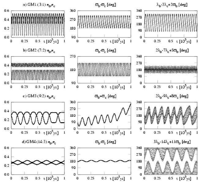
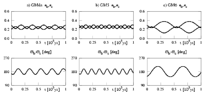
Finally, we computed the evolution of the orbital elements, for all the GM fits, given in Table 3. The results are illustrated in Figures 9 and 10 and show the complexity of the possible dynamical behaviours of the HD 160691 system that are consistent with the RV observations. The fits GM1–GM4 correspond to MMRs: 3:1, 7:2, 9:2 and 14:3, respectively. As we already mentioned, the GM3 fit is unstable although it lies close to a stable region. In this case, a curious SAR with $\theta_{1}=\varpi_{{\mbox{\scriptsize b}}}+\varpi_{{\mbox{\scriptsize c}}}$ librating about $90^{\circ}$ appears. For the other ICs, the SARs with different libration centers are also present. In the GM1 fit, corresponding to the 3:1 MMR, $\theta$ librates about $240^{\circ}$. The rest of the GM fits have $\theta$ librating about $180^{{\rm o}}$, with the semi-amplitudes as small as a few degrees (see, e.g., Figures 9d and 10b). Note also the different evolution of the eccentricities of the companions and the stabilizing influence of the MMRs.

5 Previous dynamical studies of the HD 160691 system

The HD 160691 system has attracted the attention of many researchers, most likely due to its apparent proximity to the 2:1 MMR. We have found very interesting to compare the results of previous studies with the current and still very fragmentary knowledge of its dynamics.

Shortly after the reprint by Jones et al. (2002a) had appeared, Kiseleva-Eggleton et al. (2002a) used the preliminary fit J2 to analyze its stability. Using the MEGNO technique, they found stable configurations located not very far in the parameter space from this initial condition and concluded that high eccentricity of the outermost planet $e_{\mbox{\scriptsize c}}>0.7$ is an important stabilizing factor in the HD 160691 system. A similar conclusion was quoted by these authors in (Kiseleva-Eggleton et al., 2002b). In the light of our study, these results are not quite clear for us. In our MEGNO maps, in the same ($e_{{\mbox{\scriptsize b}}},e_{{\mbox{\scriptsize c}}}$)-plane, computed for the J2 initial condition with the resolution $100\times 100$ points, there are not any stable points for $e_{{\mbox{\scriptsize c}}}>0.1$. It is illustrated in the left panel of Figure 11. All configurations with high $e_{{\mbox{\scriptsize c}}}$ are self-disrupted.

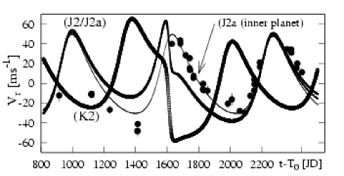
In fact, in their Table 1, Kiseleva-Eggleton et al. (2002a) quote a different time of the periastron passage of the inner planet than the one given in Jones et al. (2002a) and Jones et al. (2002b). Indeed, for IC changed this way, (see the fit K2 in Table 1), we also obtained a very extended, ridge-like zone of stability for extremely large $e_{{\mbox{\scriptsize c}}}$ (see the middle panel in Figure 11). Moreover, the initial configuration resulting from that modified IC produces the RV signal in anti-phase with the original RV curve—compare the synthetic RV curves obtained for the original and the modified IC, respectively (shown in Figure 13). Actually, it seems that all the double-Keplerian RV curves shown in Figure 13 do not describe even approximately the measurements. We did not succeed in reproducing the double-Keplerian RV curves, which have been defined by the literal values of the elements $K,n,e,\omega,T_{{\mbox{\scriptsize p}}}$ of the J2 and J2a fits (see Table 1), and calculated with the classical formulae (see Smart, 1949; Lee & Peale, 2003), as they have been shown in Jones et al. (2002b) in their Figure 3 (see our Figure 13). Only the one-Keplerian signal of the inner planet (given by the J2a fit) comes reasonably close to the RV data points. Possibly, in the original Figure 3 there is shown the one-Kepler+trend signal. Anyway, this shows that the literal elements of the outer planet in the J2 and J2a fits cannot be treated as representative for the Doppler signal of the HD 160691 .

Further, while trying to explain the differences between the results of Kiseleva-Eggleton et al. (2002a) and this paper, we noticed some stable points in their Figure 3d, located about $e_{{\mbox{\scriptsize b}}}\simeq 0.2$ which are absent in our version of this scan (see the middle panel of Figure 11). We see at least two possible explanations of this difference. The quoted authors did not specify the initial epoch of their integrations, so the different epochs can give different osculating elements and finally the MEGNO signatures. This can be also related to a “pathological” MEGNO convergence that is characteristic for collisional orbits. The Lyapunov exponent-based criterion for chaos is misleading if bodies are ejected from the system Lissauer (1999), because after the ejection the distance between the phase trajectories no longer grows exponentially. The ejected planet can stay on a distant orbit and apparently the system is bounded and regular. In such cases MEGNO can converge very close to 2, finally giving a correct identification of a stable configuration. As an example we show the results of the integration of the HD 160691 system when the J2 is changed: $e_{{\mbox{\scriptsize b}}}$ from 0.31 to 0.25 and $e_{{\mbox{\scriptsize c}}}$ from 0.8 to 0.83. The resulting MEGNO behaviour is depicted in Fig. 12. The indicator converges to 2.05 in a way characteristic for a regular system. Nevertheless, from the qualitative point of view, the resulting system is very different from the starting configuration. Thus, following Lissauer (1999), we treat the ejections as strongly chaotic phenomena, in spite of the apparent regularity of the final orbital states. Not eliminating this effect can lead to false patterns in the MEGNO stability maps that can be even recognized as narrow resonance zones. We noticed and fixed this problem with the MEGNO convergence in (Goździewski & Maciejewski, 2001).

In a recent paper, Bois et al. (2003) deal with a global analysis of the 2:1 MMR, assumed to be present in the HD 160691 system. These authors report the initial condition, which is equivalent to the J2 fit but modified in the same way as the K2 fit, and additionally, in this IC, $a_{{\mbox{\scriptsize b}}}$ has been changed from 2.3 AU to 2.381 AU. Then, using the MEGNO indicator, they analyze the dynamics of resulting planetary configurations and compare them with a similar case of the Gliese 876 2:1 MMR. In the neighborhood of the analyzed IC, there is an extended stable zone of this resonance. However, also in this case the system dynamics that has been studied, does not reproduce the RV measurements of the HD 160691 .

6 Conclusions

In this paper we attempt to verify the hypothesis stated by Jones et al. (2002b) that the linear trend apparent in the RV observations of HD 160691 is a Doppler signal of the second planetary companion. The problem we have to deal with while trying to estimate the orbital elements of the hypothetical planet, is a very short timespan of the data compared to the probable orbital period of the outer planet. Our analysis incorporates the already well recognized fact that the commonly used Keplerian model of the RV data can falsify the dynamics of the studied system. This statement has been stated by Laughlin & Chambers (2001) who pioneered the Newtonian (or “self-consistent”, i.e., incorporating the mutual interaction between companions) RV fits and have applied them to strongly interacting planets around Gliese 876. The HD 160691 system is yet another example that neglecting the full dynamics in the fitting process of the orbital elements to the RV observations leads to artifacts when the RV data permit elongated orbits and relatively small orbital distances between the planets. For the HD 160691 system, the formally best Keplerian fits describe configurations that lead to a collision of the companions during a few weeks. But such configurations are not likely as we would be observing the system just after or just before the collision event. In this sense the dynamics become an important observable that has to be taken into account with the same priority as the RV observations. To give this idea a numerical implementation, we propose a method that merges the genetic optimization algorithm with the MEGNO analysis, i.e., the examination of the orbital stability by a fast indicator. The efficiency of the MEGNO algorithm makes it possible to automate the fitting process and to gain an acceptable overall numerical efficiency of the algorithm. With such a MEGNO-penalty fitting approach, we find a number of stable orbital fits having ${(\chi^{2}_{\nu})^{1/2}}\simeq 1.48$ and an rms $\simeq 4.4~{}\mbox{ms}^{-1}$. The search have been confined to the limit of of the Jupiter-like periods of the hypothetical second planet. These configurations correspond to the low-order MMRs 3:1, 7:2 and to the neighborhoods of 14:3, 4:1, and 5:1 MMRs. This result is in excellent accord with the quasi-global, gradient search of the best Newtonian fits. It demonstrates that our algorithm reliably finds the desired, stable initial conditions that produce a synthetic Doppler signal consistent with the observations.

The current set of the RV data does not constrain the orbital elements of the outer planet. The preliminary Keplerian fits lead to a completely false dynamical representation of the HD 160691 system. Considerably more significant constraints on the possible orbital configurations and parameters of this system are provided by the dynamics. Our paper proves that the future analysis of the updated RV observations has to be driven by the full, $N$-body model of the RV observations.

Forecasting the real state of the HD 160691 system is very difficult now. The RV data permit a continuum of statistically equivalent orbital fits. However, the extensive dynamical analysis of these solutions makes it possible to give some overall characteristics of the planetary system even at this stage. If the outer planet revolves close to the inner companion, it is unlikely to maintain the system stability for large $e_{{\mbox{\scriptsize c}}}$ without a stable orbital resonance. For a distance up to about $3$ AU, the system can be locked in the low-order MMRs 3:1 or 7:2. For larger values of the semi major axis of the outer companion, up to the Jupiter-like $5.2$ AU, the system can be found in an extended zone confined to other low order MMRs, like 4:1, 5:1 or to their neighborhoods, accompanied by the SAR with semi-major axes antialigned in the exact resonance. However this type of the secular resonance does not exhaust other possibilities. Although it is speculative, the dynamical structure of this region reminds that of the HD 12661 system. Possibly, the large libration island of the SAR with the apsidal lines anti-aligned in the exact resonance can be explained by the secular theory of Lee & Peale (2003). Such a test is not straightforward to carry out because every data point in the scan represents a different initial condition and the scan data pass into the neighborhoods of the low-order MMRs. The dynamical similarity of both systems flows also from their RV signals and the masses of their host stars: if one would restrict the period of observations of the HD 12661 system to the range between JD=24511200 and JD=24511800 (see the RV data in Fischer et al., 2003), then we would see the same kind of a linear trend visible in the RV data of the HD 160691 . Also the MEGNO maps of the neighborhoods of the best stable GM fits and for the best fits of the HD 12661 system Goździewski (2003); Goździewski & Maciejewski (2003) reveal many similarities.

Because our study has mostly qualitative character, we omitted some effects in the fitting process that should be taken into account, when a more extended set of the RV data will be accessible. Specifically, we did no discuss the formal and systematic errors (e.g., from the stellar RV jitter) of the best fit parameters. This in principle could be done as in our recent paper devoted to the HD 12661 system Goździewski & Maciejewski (2003). We only considered coplanar and edge-on configurations. Incorporating the mutual interaction between planets would remove the geometrical degeneracy which does not permit to estimate the relative inclination of the orbits and the inclinations of the orbital planes Laughlin & Chambers (2001); Rivera & Lissauer (2001). Currently, the small number of measurements is an obstacle to perform such fully self-consistent fits. Hopefully, the data set will steadily grow and soon will be sufficiently large to verify of our approach and predictions.

7 Acknowledgments

Calculations in this paper have been performed on the HYDRA computer-cluster, supported by the Polish Committee for Scientific Research, Grants No. 5P03D 006 20 and No. 2P03D 001 22. This work is supported by the Polish Committee for Scientific Research, Grant No. 2P03D 001 22. K.G. wants to acknowledge the support by the N. Copernicus University, Grant No 362-A. M. K. is a Michelson Postdoctoral Fellow.

Appendix: A model of the radial velocity observations

Below we describe the Keplerian model employed in this paper. Our model differs in some details from the commonly used version which comes from the classical RV studies of stellar binaries (see e.g. Smart, 1949).

We start with the basic definitions of the Keplerian motions. The radius vector ${\mathbf{R}}(t)$ and the velocity${\mathbf{V}}(t)$ of a body moving in an elliptic orbit are given by

$${\mathbf{R}}(t)=a\left[(\cos E(t)-e)\,{\mathbf{P}}+\sqrt{1-e^{2}}\sin E(t)\,{\mathbf{Q}}\right],$$ (1)

$${\mathbf{V}}(t)=an\left[-\frac{\sin E(t)}{1-e\cos E(t)}{\mathbf{P}}+\frac{\sqrt{1-e^{2}}\cos E(t)}{1-e\cos E(t)}{\mathbf{Q}}\right],$$ (2)

where ${\mathbf{P}}={\mathbf{l}}\,\cos\omega+{\mathbf{m}}\,\sin\omega,$ ${\mathbf{Q}}=-{\mathbf{l}}\,\sin\omega+{\bf m}\cos\omega,$ and

$${\mathbf{l}}=\begin{bmatrix}\cos\Omega\\ \sin\Omega\\ 0\end{bmatrix},\qquad{\mathbf{m}}=\begin{bmatrix}-\cos i\sin\Omega\\ \phantom{-}\cos i\cos\Omega\\ \phantom{-\cos\Omega}\sin i\end{bmatrix}.$$

The eccentric anomaly $E=E(t)$ is an implicit function of time through the Kepler equation $E-e\sin E=M,$ where $M$ is the mean anomaly $M=n(t-T_{\mathrm{p}}),$, $n=2\pi/P,$ and $P$ is the orbital period of the body. The remaining parameters $a$, $e$, $\omega$, $\Omega$, $T_{p}$ are the standard Keplerian elements — semi-major axis, eccentricity, longitude of pericenter, longitude of ascending node and time of pericenter. The mean motion $n$ and the semi-major axis $a$ are connected by the relation $n^{2}a^{3}=\mu,$ where $\mu$ is the gravitational parameter. The explicit form of $\mu$ and the meaning of ${\mathbf{R}}(t)$, ${\mathbf{V}}(t)$ depend on which Kepler problem we consider (relative orbit in the two body problem, barycentric orbit, etc).

Now, let us assume that the body is a planet of mass $m$ revolving around a star of mass $m_{\star}$, and let ${\mathbf{R}}(t)$, ${\mathbf{V}}(t)$ and ${\mathbf{R}}^{\star}(t)$, ${\mathbf{V}}^{\star}(t)$ denote the barycentric radius vector and the velocity of respectively the planet and the star. By $\boldsymbol{\rho}(t):={\mathbf{R}}(t)-{\mathbf{R}}^{\star}(t)$ and $\boldsymbol{\upsilon}(t):={\mathbf{V}}(t)-{\mathbf{V}}^{\star}(t)$ we denote the relative radius vector and velocity of the planet. From the definition of the center of mass we have

$${\mathbf{R}}^{\star}(t)=-\frac{m}{m_{\star}}{\mathbf{R}}(t)=-\frac{m}{m_{\star}+m}\boldsymbol{\rho}(t),$$ (3)

$${\mathbf{V}}^{\star}(t)=-\frac{m}{m_{\star}}{\mathbf{V}}(t)=-\frac{m}{m_{\star}+m}\boldsymbol{\upsilon}(t),$$ (4)

We choose the barycentric reference frame in such a way that its third axis has the direction of the vector from the observer to the mass center of the system. Hence the radial velocity of the star is the third component of its barycentric velocity, $v^{\star}_{\mathrm{r}}(t):=V^{\star}_{3}(t)$. Now, we can express $v^{\star}_{\mathrm{r}}(t)$ in terms of Keplerian elements of the planet:

$$v^{\star}_{\mathrm{r}}(t)=-L\left[\frac{\sqrt{1-e^{2}}\cos E(t)\cos\omega-\sin E(t)\sin\omega}{1-e\cos E(t)}\right],$$ (5)

where the explicit form of $L$ as well as all Keplerian elements depend on our choice of the planetary orbit .

In the case of the barycentric orbit $L=\sigma an\sin i,$ where $\sigma=m/m_{\star}$ and $\mu=Gm_{\star}^{3}/(m_{\star}+m)^{2}.$ For the relative orbit the form of $L$ is the same, with $\sigma=m/(m_{\star}+m)$ and $\mu=G(m_{\star}+m).$ It should be noted here that not only semi-major axes calculated for the barycentric and the relative orbit of the planet are different but also the eccentricities may be different.

When performing the least-squares fit to the radial velocity data both parameterizations give the same results (of course, after an appropriate transformation). It is not so clear when we have more than one planet. Typically, the radial velocity of the star is modeled in barycentric coordinates as a sum of terms (5) calculated for each planet (but the semi-major axis of planet’s orbits and the lower limits on their masses are then often given for the relative orbits which is a strange mismatch for systems containing more than one planet). However in barycentric coordinates, even if we assume that the planets do not interact directly, their orbits are not Keplerian. In such a case, the companions still interact indirectly via the host star. Only in the Jacobi coordinates the direct and indirect effects of the mutual interactions between planets are much smaller than the leading terms of the star-planet interactions. Note that this is a well known fact—for instance, the already classic symplectic integrators by Wisdom & Holman (1991) heavily rely on the use of Jacobi coordinates. Recently, this has been analyzed in the context of the RV data modeling in by Lee & Peale (2003). They point out that the double-Keplerian orbital fits have to be expressed in Jacobi coordinates and not in the barycentric coordinates. Further, using the “classic” approach, we are not allowed to calculate the masses of the companions by using the same formulas as for the barycentric motion of the two bodies. There is not any well defined gravitational parameter if the RV fits of a multi-planetary system are represented directly in terms of the barycentric Keplerian elements. Amazingly, these actually quite obvious conclusions are relevant to tens of already published papers on extrasolar planets discovered through precise RVs! It is worth to note that in recent years, in the extrasolar planet field it has been properly approached in the case of PSR B1257+12 planetary system (Konacki et al., 2000). Lee & Peale (2003) give a clear explanation of the problem in the context of RV measurements.

For simplicity, let us assume that we have two planets with the masses $m_{1}$ and $m_{2}$. Their barycentric radius vectors an velocities we denote by ${\mathbf{R}}_{i}$, ${\mathbf{V}}_{i}$, $i=1,2$. The Jacobi coordinates and velocities ${\mathbf{r}}_{i}$, ${\mathbf{v}}_{i}$ of the planets are defined in the following way

$${\mathbf{r}}_{1}:={\mathbf{R}}_{1}-{\mathbf{R}}^{\star},\qquad{\mathbf{r}}_{2}:={\mathbf{R}}_{2}-\frac{1}{m_{\star}+m}\left(m_{\star}{\mathbf{R}}^{\star}+m_{1}{\mathbf{R}}_{1}\right),$$ (6)

$${\mathbf{v}}_{1}:={\mathbf{V}}_{1}-{\mathbf{V}}^{\star},\qquad{\mathbf{v}}_{2}:={\mathbf{V}}_{2}-\frac{1}{m_{\star}+m}\left(m_{\star}{\mathbf{V}}^{\star}+m_{1}{\mathbf{V}}_{1}\right).$$ (7)

Thus, ${\mathbf{r}}_{1}$ is the position of $m_{1}$ relative to $m_{\star}$, and ${\mathbf{r}}_{2}$ is the position of $m_{2}$ with respect to the center of mass of $m_{\star}$ and $m_{1}$. In terms of the Jacobi coordinates we have

$${\mathbf{R}}^{\star}=-\sigma_{1}{\mathbf{r}}_{1}-\sigma_{2}{\mathbf{r}}_{2},\quad{\mathbf{V}}^{\star}=-\sigma_{1}{\mathbf{v}}_{1}-\sigma_{2}{\mathbf{v}}_{2},$$ (8)

where $\sigma_{1}=m_{1}/(m_{\star}+m_{1})$, $\ \sigma_{2}=m_{2}/(m_{\star}+m_{1}+m_{2}).$ As we already mentioned, in the Jacobi coordinates we can consider the three body problem as a perturbation of two the two body models: the planet $m_{1}$ plus the star, and the planet $m_{2}$ plus a fictitious point of mass $m_{\star}+m_{1}$. Thus, approximating the planetary motion by these two problems, we obtain that $v^{\star}_{\mathrm{r}}(t)=-L_{1}f_{1}(t)-L_{2}f_{2}(t)$, where $L_{k}=\sigma_{k}a_{k}n_{k}\sin i_{k}$, $k=1,2$, $\mu_{1}=G(m_{\star}+m_{1})$, $\mu_{2}=G(m_{\star}+m_{1}+m_{2})$, and

$$f_{k}(t)=\frac{\sqrt{1-e_{k}^{2}}\cos E_{k}(t)\cos\omega_{k}-\sin E_{k}(t)\sin\omega_{k}}{1-e_{k}\cos E_{k}(t)}.$$ (9)

Table 1: Orbital parameters of the HD 160691 system, adopted from data published in Jones et al. (2002a) (J2), Jones et al. (2002b) (J2a), and used in Kiseleva-Eggleton et al. (2002a)(K2). The mass of the central star is equal to $1.08~{}\mbox{M}_{\sun}$.

	J2		J2a		K2
Orbital parameter / planet	b	c	b		b	c
$\mbox{m}_{{\mbox{\scriptsize pl}}}\sin i$ [M${}_{{\mbox{\scriptsize J}}}$]	1.7	(1.0)	1.7	($>$1.5)	1.7	1.0
$a$ [AU]	1.5	(2.3)	1.5	($>$2.5)	1.5	2.3
$P$ [d]	638	(1300)	637	(1500)	638	1300
$e$	0.31	(0.8)	0.31	(0.8)	0.31	0.8
$\omega$ [deg]	320	(99)	320	(99)	320	99
$T_{{\mbox{\scriptsize p}}}$ [HJD-2400000]	50958	(51613)	50959	(51613)	50698	51613
K [$\mbox{ms}^{-1}$]	40	(34.2)	40	(34)
rms [$\mbox{ms}^{-1}$]	5.42	(5)	5.28	(5)

Table 2: The orbital parameters of the HD 160691 system derived from the double-Keplerian Levenberg-Marquardt fit (JK2), the genetic fit (GA2), and the Levenberg-Marquardt self-consistent Newtonian fit (NL2). The JK2 and GA2 parameters are related to Jacobi coordinates; the NL2 fit is given in the astrocentric Keplerian elements at the epoch of the first observation ($t_{0}\equiv$ JD2450915.2911). The mass of the parent star is equal to $1.08~{}\mbox{M}_{\sun}$. See the Appendix for an explanation of the symbol $L$.

	JK2		GA2		NL2
Orbital parameter /planet	b	c	b	c	b	c
$\mbox{m}_{{\mbox{\scriptsize pl}}}\sin i$ [M${}_{{\mbox{\scriptsize J}}}$]	1.68	2.09	1.69	1.44	1.68	2.18
$L$ [$\mbox{ms}^{-1}$]	38.2	34.7	38.3	23.5
$a$ [AU]	1.449	2.708	1.460	2.813	1.437	2.724
$P$ [d]	612.4	1563.6	619.43	1655.5
$e$	0.348	0.864	0.326	0.700	0.340	0.879
$\omega$ [deg]	141.0	311.4	140.1	293.4	141.7	314.4
$T_{{\mbox{\scriptsize p}}}$ [JD-2450000]	393.4	940.5	2231.2	2601.1
$M(t_{0})$ [deg]	306.8	354.2	315.2	353.4	307.7	354.7
$V_{0}$ [$\mbox{ms}^{-1}$]	-10.9		-6.6		-11.0
${(\chi^{2}_{\nu})^{1/2}}$	1.38		1.41		1.40
rms [$\mbox{ms}^{-1}$]	3.9		4.0		4.0

Table 3: Newtonian, genetic fits with the MEGNO penalty test. Osculating, astrocentric Keplerian elements are given for the the epoch of the first observation (JD=2450915.2911).

Fit	Planet	$V_{0}$	${(\chi^{2}_{\nu})^{1/2}}$	rms	$m_{{\mbox{\scriptsize pl}}}\sin i$	$a$	$e$	$\omega$	$M$	Note
		[$\mbox{ms}^{-1}$]		[$\mbox{ms}^{-1}$]	[$m_{{\mbox{\scriptsize J}}}$]	[AU]		[deg]	[deg]
GM1	a	-7.2	1.49	4.40	1.69	1.493	0.287	133.0	344.1
	b				1.26	3.117	0.457	290	33.6	SAR ($240^{\circ}$)
stable	b				1.26	3.100	0.457	290	33.6	3:1 MMR
GM2	a	-5.1	1.47	4.35	1.72	1.493	0.284	133.2	344.2	7:2 MMR
(best)	b				1.32	3.444	0.377	302.1	26.0	SAR ($180^{\circ}$)
GM3	a	-7.4	1.48	4.40	1.70	1.493	0.284	133.5	343.4	$\simeq$ 9:2 MMR
	b				1.71	4.048	0.304	307.1	53.4
GM4	a	-4.1	1.48	4.40	1.70	1.491	0.283	135.9	340.0	14:3 MMR
	b				1.52	4.178	0.250	325.1	24.4	SAR ($180^{\circ}$)
GM4a	a	-4.3	1.49	4.35	1.73	1.492	0.285	137.9	338.7
	b				1.44	4.144	0.210	332.3	17.5	SAR ($180^{\circ}$)
GM5	a	-3.9	1.48	4.36	1.74	1.494	0.289	134.8	343.4
	b				1.52	4.305	0.236	329.1	25.0	SAR ($180^{\circ}$)
GM6	a	-3.7	1.48	4.33	1.73	1.493	0.289	135.4	342.1
	b				1.67	4.773	0.220	347.8	16.3	SAR ($180^{\circ}$)

Figure 1: Stability MEGNO-maps in the ($a_{{\mbox{\scriptsize c}}},e_{{\mbox{\scriptsize c}}})$-plane for different initial orbital phases of the outer planet. The orbital elements are related to the J2 fit, see Table 1. The left column corresponds to the nominal $\omega_{{\mbox{\scriptsize c}}}$ of the outer planet. Some of the stable areas (shaded) corresponding to the mean motion resonances are labeled. The resolution of the plots is $240\times 100$ points.

Figure 2: Evolution of the Keplerian, astrocentric elements in the 2:1 MMR (the left column, $a_{{\mbox{\scriptsize c}}}=2.36$ AU, $e_{{\mbox{\scriptsize c}}}=0.792$, $M_{{\mbox{\scriptsize c}}}=90^{\circ}$) and in the 3:1 MMR (the right column, $a_{{\mbox{\scriptsize c}}}=3.1416667$AU, $e_{{\mbox{\scriptsize c}}}=0.9801$, $M_{{\mbox{\scriptsize c}}}=90^{\circ}$). Note that these parameters are modified orbital parameters of the nominal J2 fit, interpreted here as the osculating Keplerian elements at the epoch of the periastron passage of the outer planet. They are localized in the zones of stability shown in Figure 1.

Figure 3: Panel a) is for the function ${(\chi^{2}_{\nu})^{1/2}}(P_{{\mbox{\scriptsize c}}},e_{{\mbox{\scriptsize c}}})$ of the RV model which incorporates one planet in a Keplerian orbit and a linear trend. Contour levels are: 1.5, 2.0, 2.5. Panel b) is for the double-Keplerian model of the RV data and its ${(\chi^{2}_{\nu})^{1/2}}(P_{{\mbox{\scriptsize c}}},e_{{\mbox{\scriptsize c}}})$. Contour levels are: 1.40, 1.45, 1.5. Panel c) is for the logarithm of the absolute difference in ${(\chi^{2}_{\nu})^{1/2}}(P_{{\mbox{\scriptsize c}}},e_{{\mbox{\scriptsize c}}})$ between the double-Keplerian model and the Newtonian model of the RV data. The best double-Keplerian solution is marked by the the intersection of the two straight lines. Panel d) is a map of ${(\chi^{2}_{\nu})^{1/2}}$ computed from the self-consistent Newtonian model of the dynamics when the orbital parameters are fitted by the gradient method, starting from the best double-Keplerian solutions (see the text for more details). Contour levels are: 1.40, 1.45, 1.5. The resolution of the plots is $200\times 100$ points.

Figure 4: Dynamical scans of the ${(\chi^{2}_{\nu})^{1/2}}$-map of the best double-Keplerian fits (Figure 3b). The orbital parameters of these fits have been mapped to the osculating astrocentric elements at the epoch of the first observation. The top left panel (a) is for the MEGNO, the top right panel (b) is for the maximum eccentricity of the inner companion. The bottom left panel (c) is for the maximum of $\theta=\varpi_{{\mbox{\scriptsize b}}}-\varpi_{{\mbox{\scriptsize c}}}$ centered about $0^{\circ}$, the bottom right panel (d) is for $\theta$ centered about $180^{\circ}$. The integration time is about $10^{4}$ periods of the outer planet. The thick curve represents the planetary collision line given through $a_{{\mbox{\scriptsize b}}}(1+e_{{\mbox{\scriptsize b}}})=a_{{\mbox{\scriptsize c}}}(1-e_{{\mbox{\scriptsize c}}})$, where $a_{{\mbox{\scriptsize b}}}=1.49$ AU and $e_{{\mbox{\scriptsize c}}}=0.31$ are fixed. Approximate positions of the lowest order MMRs, relevant to the discussion, are labeled. The resolution of the plots is $200\times 100$ points.

Figure 5: The top panels show a comparison of the synthetic RV curves, obtained from the best double-Keplerian fits (JK2 and GA2, $V_{{\mbox{\scriptsize r}}}^{{\mbox{\scriptsize J}}}$), and from the numerical integration incorporating the double-Keplerian solutions as the osculating elements at the epoch of the first observation ($V_{{\mbox{\scriptsize r}}}^{{\mbox{\scriptsize N}}}$). The left column is for the best JK2 fit, the right column is for the best genetic fit GA2 (see Table 2). In order to make the comparison more transparent, the bottom panels shows the appropriate differences between the Keplerian and Newtonian synthetic RV signals. Time is given in Julian Days, with $T_{0}=$JD2450000.

Figure 6: Synthetic RV curves for the best self-consistent fits obtained by scanning the parameters space with the Levenberg-Marquardt algorithm (NL2) and by the genetic algorithm combined with the MEGNO signature (GM2). The best fit parameters are given in Tables 2 and 3. Time is given in Julian Days, with $T_{0}=$JD2450000.

Figure 7: A representation of the best self-consistent Newtonian fits obtained by the gradient method in the $(a_{{\mbox{\scriptsize c}}},e_{{\mbox{\scriptsize c}}})$-plane of astrocentric, osculating elements. The initial epoch is the Julian Date of the first observation. The best double-Keplerian fits have been used as the starting points for the gradient method (see the text for more details). The dots mark the fits which have ${(\chi^{2}_{\nu})^{1/2}}<1.5$, $e_{{\mbox{\scriptsize b}}}$, $e_{{\mbox{\scriptsize c}}}$ stand for the eccentricity of the inner and the outer companion, respectively. The large, filled circles mark these $(a_{{\mbox{\scriptsize c}}},e_{{\mbox{\scriptsize c}}})$ of the fits that lead to a stable, quasi-periodic evolution of the planetary system. For these fits $|\langle Y\rangle-2|<0.05$. Crosses mark the initial parameters found by the MEGNO-penalty fits (Table 3).

Figure 8: Stability maps in the ($a_{{\mbox{\scriptsize c}}},e_{{\mbox{\scriptsize c}}})$-plane for the best genetic fits GM1–GM6 (Table 3), obtained by applying the MEGNO penalty algorithm. The fitted parameters, given in Table 3, are marked by the intersection of the two lines. The resolution of these scans is $160\times 100$ data points.

Figure 9: Evolution of the orbital elements for the subsequent GM solutions (rows). For the GM1 solution $a_{{\mbox{\scriptsize c}}}=3.1$AU. See also Table 3.

Figure 10: Evolution of the orbital elements in the GM fits (columns). See also Table 3.

Figure 11: Stability maps in the $(e_{{\mbox{\scriptsize b}}},e_{{\mbox{\scriptsize c}}})$-plane: the left panel is for the J2 fit from Jones et al. (2002a), the middle panel is for the initial condition from Kiseleva-Eggleton et al. (2002a) (the fit K2). The right panel is for the fit K2 and it illustrates which systems are disrupted by a collision or ejection of a planet. Such disrupted systems are marked with different gray codes: 1 is for $e_{{\mbox{\scriptsize b}}}>0.999$, 2 is for $e_{{\mbox{\scriptsize c}}}>0.999$, 3 is for $a_{{\mbox{\scriptsize b}}}>10$ AU, 4 is for $a_{{\mbox{\scriptsize b}}}>10$ AU. Note the short timescale of the instabilities: the time of integration is at most equal to about $10^{4}$ periods of the outer companion. The resolution of the left plot is $100\times 100$, for the two other plots it is equal to $190\times 190$ data points.

Figure 12: An example of a misleading MEGNO convergence for a case of a self-disrupting system. The left panel is for the initial condition J2 (Table 1) modified in such a way that $e_{{\mbox{\scriptsize b}}}=0.29$ and $e_{{\mbox{\scriptsize c}}}=0.83$. A collision after about $14$ days disrupts the system. The right panel is for MEGNO. The indicator converges to $\simeq 2.05$.

Figure 13: Keplerian RV curves for the initial conditions given in Jones et al. (2002a) (J2/J2a) and Kiseleva-Eggleton et al. (2002a) (K2). Small, filled circles are for the J2 and J2a fits. Open circles are for the K2 initial condition (see Table 1). In all these cases, the RV offset is unspecified and it has been set to $V_{0}=0~{}\mbox{ms}^{-1}$. Large, filled circles are for the RV measurements published in Jones et al. (2002b). Thin line is for the RV corresponding to the signal of the inner planet only (its elements are given by the J2a fit). Note that the RV signals have been calculated using the true anomaly parameterization of the RV signal (see the Appendix for explanation). Time is given in Julian Days, with $T_{0}=$JD2450000.

References

- Bois et al. (2003) Bois, E., Kiseleva-Eggleton, L., Rambaux, N., & Pilat-Lohinger, E. 2003, ApJ, astro-ph/0301528
- Butler et al. (1999) Butler, R. P., Marcy, G. W., Fischer, D. A., Brown, T. M., Contos, A. R., Korzennik, S. G., Nisenson, P., & Noyes, R. W. 1999, ApJ, 526, 916
- Butler et al. (2001) Butler, R. P., Tinney, C. G., Marcy, G. W., Jones, H. R. A., Penny, A. J., & Apps, K. 2001, ApJ, 555, 410
- Charbonneau (1995) Charbonneau, P. 1995, ApJS, 101, 309
- Cincotta & Simó (2000) Cincotta, P. M. & Simó, C. 2000, A&AS, 147, 205
- Fischer et al. (2003) Fischer, D. A., Marcy, G. W., Butler, R. P., Vogt, S. S., Henry, G. W., Pourbaix, D., Walp, B., Misch, A. A., & Wright, J. 2003, ApJ, 586, 1394
- Goździewski (2003) Goździewski, K. 2003, A&A, 398, 1151
- Goździewski & Maciejewski (2003) Goździewski, K. & Maciejewski, A. J. 2003, ApJ, 586, L153
- Goździewski (2003) Goździewski, K. 2003, A&A, 398, 315
- Goździewski et al. (2002) Goździewski, K., Bois, E., & Maciejewski, A. 2002, MNRAS, 332, 839
- Goździewski et al. (2001) Goździewski, K., Bois, E., Maciejewski, A., & Kiseleva-Eggleton, L. 2001, A&A, 378, 569
- Goździewski & Maciejewski (2001) Goździewski, K. & Maciejewski, A. 2001, ApJ, 563, L81
- Hadjidemetriou (2002) Hadjidemetriou, J. D. 2002, Celestial Mechanics and Dynamical Astronomy, 83, 141
-
Hairer & Wanner (1995)
Hairer, E. & Wanner, G. 1995,
http://www.unige.ch/math/folks/hairer/ - Ji et al. (2002) Ji, J., Li, G., & Liu, L. 2002, ApJ, 572, 1041
- Jiang-Hui et al. (2002) Jiang-Hui, J., Lin, L., Kinoshita, H., & Nakai, H. 2002, Chinese Astronomy and Astrophysics, 26, 379
- Jones et al. (2002a) Jones, H., Butler, P., Marcy, G., Tinney, C., Penny, A., C., M., & B., C. 2002a, MNRAS, astro-ph/0206216
- Jones et al. (2002b) Jones, H. R. A., Paul Butler, R., Marcy, G. W., Tinney, C. G., Penny, A. J., McCarthy, C., & Carter, B. D. 2002b, MNRAS, 337, 1170
- Kiseleva-Eggleton et al. (2002a) Kiseleva-Eggleton, L., Bois, E., Rambaux, N., & Dvorak, R. 2002a, ApJ, 578, L145
- Kiseleva-Eggleton et al. (2002b) Kiseleva-Eggleton, L., Bois, E., Rambaux, N., Dvorak, R., & Rivera, E. J. 2002b, American Astronomical Society Meeting, 201
- Konacki et al. (2000) Konacki, M., Maciejewski, A. J., & Wolszczan, A. 2000, ApJ, 544, 921
- Laughlin & Chambers (2001) Laughlin, G. & Chambers, J. E. 2001, ApJ, 551, L109
- Laughlin & Chambers (2002) —. 2002, AJ, 124, 592
- Lee & Peale (2002) Lee, M. H. & Peale, S. J. 2002, ApJ, 567, 596
- Lee & Peale (2003) —. 2003, ApJ, submitted
- Lissauer (1999) Lissauer, J. J. 1999, Rev. Mod. Phys., 71, 835
- Marcy et al. (2002) Marcy, G. W., Butler, R. P., Fischer, D. A., Laughlin, G., Vogt, S. S., Henry, G. W., & Pourbaix, D. 2002, ApJ, 581, 1375
- Murray & Holman (2001) Murray, N. & Holman, M. 2001, Nature, 410, 773
- Press et al. (1992) Press, W. H., Teukolsky, S. A., Vetterling, W. T., & Flannery, B. P. 1992, Numerical Recipes in C. The Art of Scientific Computing (Cambridge Univ. Press)
- Rivera & Lissauer (2001) Rivera, E. J. & Lissauer, J. J. 2001, ApJ, 402, 558
- Robutel & Laskar (2001) Robutel, P. & Laskar, J. 2001, Icarus, 152, 4
- Smart (1949) Smart, W. M. 1949, Text-Book on Spherical Astronomy (Cambridge Univ. Press)
- Stepinski et al. (2000) Stepinski, T. F., Malhotra, R., & Black, D. C. 2000, ApJ, 545, 1044
- Wisdom & Holman (1991) Wisdom, J. & Holman, M. 1991, AJ, 102, 1528