Tracking and coupled dark energy as seen by WMAP

Abstract

The satellite experiment WMAP has produced for the first time a high-coverage, high-resolution survey of the microwave sky, releasing publicly available data that are likely to remain unrivalled for years to come. Here we compare the WMAP temperature power spectrum, along with an exhaustive compilation of previous experiments, to models of dark energy that allow for a tracking epoch at the present, deriving updated bounds on the dark energy equation of state and the other cosmological parameters. Moreover, we complement the analysis by including a coupling of the dark energy to dark matter. The main results are: a) the WMAP data alone constrain the equation of state of tracking dark energy to be $w_{\phi}<-0.67(-0.49)$ to 68%(95%) (confining the analysis to $w_{\phi}>-1$), which implies for an inverse power-law potential an exponent $\alpha<0.99(2.08)$; b) the dimensionless coupling to dark matter is $|\beta|<0.07(0.13)$. Including the results from the supernovae Ia further constrains the dark energy equation of state.

I Introduction

The WMAP satellite has just released the first full sky maps produced after more than one year of operation (Bennett et al. 2003). These data mark an important step in cosmology: they represent in fact the first publicly available multi-band high-resolution full-sky survey of the microwave sky. The WMAP survey is likely to remain the highest-quality CMB temperature anisotropy survey until the launch of the Planck satellite not earlier than 2007. Although the exercise of parameter fitting with each new experiment has produced in the last few years a copious literature, the new WMAP data are certainly on a class of its own and deserve to be taken fully into account. Here we address the question of what the first year of WMAP data can tell us about the property of dark energy.

Five years after the first observational hints about the existence of a dominant component of unclustered matter with negative pressure (Riess et al. 1998, Perlmutter et al. 1999), the so-called dark energy or quintessence (Wetterich 1988; Ratra & Peebles 1988; Frieman et al. 1995; Ferreira & Joyce 1997; Caldwell et al. 1998), there are still very few indications as to its nature. The main reason, perhaps, is that we lack any specific theoretical suggestion on the properties of the dark energy, i.e. on its self-interaction potential and on how it interacts with the other cosmological components. Several works have tried to constrain dark energy models with pre-WMAP high resolution CMB data, leading to bounds on the dark energy equation of state. Unless strong priors on the other cosmological parameters are imposed, however, these bounds turned out to be rather weak. In particular, the Hubble constant is strongly degenerated with the dark energy present equation of state, $w_{\phi}$ (Huey et al. 1999). For instance, with a flat prior $h\in(0.45-0.9)$, Amendola et al. (2002) found that essentially all values $w_{\phi}<0$ were allowed, while $w_{\phi}=-0.65\pm 0.2$ if $h=0.65\pm 0.05$. Similarly, adopting the HST value $h=0.72\pm 0.08$ (Freedman et al. 2001) and using updated data Melchiorri et al. (2002) found $w_{\phi}\in(-0.45,-1.81)$ at 95% c.l. (they included also values $w_{\phi}<-1$). Other works that addressed the same issue includes Corasaniti & Copeland (2002), Baccigalupi et al. (2002). With pre-WMAP data, only the imposition of a low value of $h$ (e.g. $h<0.7$) could allow to distinguish dynamical dark energy from a pure cosmological constant (or, more precisely, from a fluid possessing an equation of state close to $w_{\phi}=-1$ at the present).

In reality, all the constraints for CMB presented in the literature on the dark energy equation of state are necessarily somewhat model-dependent, since the fundamental quantity, namely the angular-diameter distance to last scattering, in general depends on $w_{\phi}$ through two integrals over the cosmic evolution that do not allow to distinguish among different parameters along degeneracy curves. Although at low $\ell$s the geometric degeneracy could in principle be broken by the ISW effect, the cosmic variance and the weakness of the effect make this possibility unrealistic in most cases. Here, as in several other works on the topics, we restrict therefore our attention to two classes of models which are at the same time general (in the sense of covering most modelizations) and simple. The initial conditions are choosen so that the trajectories reach the tracking solutions (notice that off-tracking solutions are indistinguishable from a cosmological constant). First, we consider dark energy as a scalar field with inverse power-law potentials $V\sim\phi^{-\alpha}$ (Ratra & Peebles 1988), which recovers the exponential potentials for large values of $\alpha$ ; in this case, the equation of state at the present is roughly constant

$$w_{\phi}=\frac{p_{\phi}}{\rho_{\phi}}\approx-\frac{2}{\alpha+2}$$ (1)

due to the tracking mechanism (Steinhardt et al. 1999). This approximates also the cases in which the dark energy is a perfect fluid with constant $w_{\phi},$ since the angular size of the acoustic horizon depend on the equation of state only, and includes also the cases in which $w_{\phi}$ is the $\Omega_{\phi}$-weighted average of a slowly-varying function $\hat{w}_{\phi}(a)$ (see e.g. Doran et al. 2001).

The WMAP team analysed their power spectrum including dark energy with a constant equation of state (and no coupling). They found for the equation of state $w_{\phi}<-0.5$ with CMB data alone and $w_{\phi}<-0.78$ including supernovae (Spergel et al. 2003). Although dark energy with an inverse power-law potential has an equation of state which is constant only near the present epoch, we will recover very similar results for this class of models, as expected.

In the second class we include models of dark energy coupled to dark matter (Amendola 2000; Amendola et al. 2002). This class of models, in which we include the conformally related Brans-Dicke Lagrangians, has been widely studied in the context of dark energy (Uzan 1999, Chiba 1999, Chen & Kamionkowski 1999, Baccigalupi et al. 2000, Holden & Wands 2000, Chimento et al. 2000, Billyard & Coley 2000, Bean & Magueijo 2000, Esposito-Farese & Polarsky 2001, Sen & Sen 2001, Gasperini et al. 2002, Pietroni 2002) It is important to stress that the behavior of coupled dark energy cannot be modeled simply by some choice of the equation of state for $\phi$ because the interaction induces on dark matter an effective equation of state different from zero. In this case dark energy mediates a long-range scalar interaction that modifies the gravity felt by dark matter particles through a Yukawa-type term (Damour et al. 1990). On Newtonian scales, the interaction simply renormalizes Newton’s constant for dark matter

$$G^{\prime}=G(1+\frac{4\beta^{2}}{3})$$ (2)

where $\beta$ is the dimensionless coupling, while the baryons remain uncoupled (or very weakly coupled, as required by experimental constraints, see e.g. Hagiwara et al. 2002). Then, dark energy effectively violates the equivalence principle, but in a way that is locally unobservable. For as concerns us, the main effect of the coupling is to induce an exchange of energy between the two dominating dark components so that, after equivalence but before acceleration, the universe enters a regime in which not only the equation of state (as in the tracking case) but also the density parameters $\Omega_{m},\Omega_{\phi}$ are constant. In Amendola (2001) this regime was called $\phi$MDE, to remark the fact that matter is not the only dominating component. This epoch ends when the dark energy enters the tracking regime, the potential energy takes over and accelerates the expansion. During $\phi$MDE we have $\Omega_{\phi}=4\beta^{2}/3$ and an effective equation of state for the coupled fluid dark matter/dark energy

$$w_{e}=\frac{p_{tot}}{\rho_{tot}}=\frac{4\beta^{2}}{9}$$ (3)

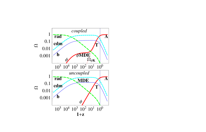
Note that this behavior is an example of “early quintessence” (Caldwell et al. 2003), in which the dark energy density is not negligible at last scattering. Scope of this paper is to constrain both equations of state, the present one, $w_{\phi}$ and the past one, $w_{e}$. This will put limits on the two “fundamental” parameters $\alpha,\,\beta$. A value $\alpha\not=0$ would imply that the dark energy is not a pure cosmological constant, while a value $\beta\not=0$ would imply a large-scale violation of the equivalence principle. In the following we will use interchangeably the parameters $w_{\phi},w_{e}$ or $\alpha,\,\beta$. In Fig. 1 we compare the background trajectories for the uncoupled ($\beta=0$) and coupled ($\beta=0.1$) cases, assuming $\alpha=1,\omega_{b}=0.02,\omega_{c}=0.1,h=0.7$. Notice the plateau of constant $\Omega_{\phi}$ in the coupled model.

We start with assuming no coupling, $\beta=0$, and varying $w_{\phi}$ along with $h,\omega_{c}=\Omega_{c}h^{2},\omega_{b}=\Omega_{b}h^{2}$ and the slope $n_{s}$ of the primordial fluctuations. Then we include $\beta$ and constrain both $w_{\phi}$ and $w_{e}$. We assume a flat space throughout. Notice that our $\Omega_{c}$ refers to cold dark matter only, so that the total matter content is $\Omega_{m}=\Omega_{b}+\Omega_{c}$.

Figure 1: Behavior of the energy densities for the coupled ($\beta=0.1$, top) and uncoupled ($\beta=0$, bottom) model. Notice, in the coupled case, the $\phi$MDE in which $\Omega_{\phi}$ is almost constant and dominated by the kinetic energy of the scalar field. The label $T$ denotes the tracking behavior, the label $A$ denotes the final future attractor.

II Data and method

The class of models considered in this paper is the same as in Amendola et al. (2002). We compare the models to the combined power spectrum estimated by WMAP (Hinshaw et al. 2003). To derive the likelihood we adopt a version of the routine described in Verde et al. (2003), which takes into account all the relevant experimental properties (calibration, beam uncertainties, window functions, etc). Since the likelihood routine employs approximations that work only for spectra not too far from the data, we run it only for models whose $\chi^{2}$ is less than four times the degrees of freedom. We experimented with increasing the $\chi^{2}$ cut and found no important variations.

We also compare the data to the whole set of pre-WMAP data. To do this, we use the power spectrum provided by Wang, Tegmark and Zaldarriaga (2002), which is a compression of essentially all the available data up to mid-2002 in 25 $\ell$-bins from $\ell=2$ to $\ell=1700$, complete of correlation matrix and window functions (calibration and beam uncertainty are included in the correlation matrix). The main entries in this compilation are COBE (Bennett et al. 1996), Boomerang (Netterfield et al. 2002), DASI (Halverson et al. 2002), Maxima (Lee et al. 2002), CBI (Pearson et al. 2002), VSA (Scott et al. 2002). To this we add Archeops (Benoit et al. 2002) with its correlation matrix, window functions, beam and calibration uncertainties. For the pre-WMAP data we assumed no reionization ($\tau=0$) because this was the best fit before WMAP.

For the pre-WMAP data we integrated out analytically the calibration and beam uncertainties and the overall normalization. Let us denote with $N_{e},\sigma_{e},\sigma_{w,e}$ the correlation matrix, the calibration uncertainty and the beam uncertainty, respectively, of the $e$-th experiment, and with $I_{e}=\{1,1,1,...,\}$ a vector of dimension equal to the number of bins in the $e$-th experiment. Moreover, let $C_{\ell,t}\prime$ be the theoretical CMB spectrum binned in the $\ell$-th bin with the experimental window function. Then one gets the remarkably simple likelihood function (see Appendix)

$$L=\exp\left[-\frac{1}{2}\left(\gamma-\frac{\beta^{2}}{\alpha}\right)\right]$$ (4)

where

$$\alpha = \sum_{e}I_{e}^{T}M_{e}^{-1}I_{e}$$ (5)

$$\beta = \sum_{e}I_{e}^{T}M_{e}^{-1}(Z_{t}-Z_{d})$$ (6)

$$\gamma = \sum_{e}(Z_{t}-Z_{d})^{T}M_{e}^{-1}(Z_{t}-Z_{d})$$ (7)

where the matrix $M_{e}$ is

$$M_{e}=(C_{\ell,d}^{T}C_{\ell,d})^{-1}N_{e}+\sigma_{e}^{2}I_{e}^{T}I_{e}+\sigma_{w,e}A^{T}A$$ (8)

and where $Z_{t}=\log(C_{\ell,t}\prime)$ and $Z_{d}=\log C_{\ell,d}$ and where the vector $A$ expresses the dependence on $\ell$ of the beam uncertainty (in the case of a Gaussian beam, $A=\{\ell_{1}^{2},\ell_{2}^{2},...,\ell_{i}^{2}\}$). This is the likelihood we use for the pre-WMAP data.

Our theoretical model depends on two scalar field parameters, four cosmological parameters and the overall normalization:

$$\alpha,\beta,n_{s},h,\omega_{b},\omega_{c},A.$$ (9)

As anticipated, to save computing time we found it necessary to restrict the analysis to a flat space; moreover, we fixed the optical depth to $\tau=0.17$, the best fit found by MAP (Spergel et al. 2003). We derived the likelihood also for $\tau=0.1$ and found no significative differences for as concerns the two dark energy parameters $\alpha,\,\beta$. The initial conditions for the scalar field are found iteratively for each set of cosmological parameters. The overall normalization has been integrated out numerically. Since $\alpha,\beta$ determine uniquely the present and past equations of state, we will present the likelihood also as function of $w_{\phi},w_{e}$ . We calculate the theoretical $C_{\ell,t}$ spectra by a modified parallelized CMBFAST (Seljak & Zaldarriaga 1996) code that includes the full set of coupled perturbation equations (see Amendola 2000 and Amendola & Tocchini-Valentini 2001). The other parameters are set as follows: $T_{cmb}=2.726K,$ $Y_{He}=0.24,N_{\nu}=3.04$.

We evaluated the likelihood on two grids of roughly $50,000$ models each (for each normalization): a sparse grid that covers a broad volume was used as a preliminary exploration; a second denser grid centered on the peaks of the first was then used for the actual calculations. For the first grid we adopted the following top-hat broad priors: $\beta\in(0,0.3),$ $\quad\alpha\in(0.25,20),\quad$ $n_{s}\in(0.8,1.2),$ $\quad\omega_{b}\in(0.005,0.04),\quad$ $\omega_{c}\in(0.05,0.3)$ . For the Hubble constant we adopted the top-hat prior $h\in(0.5,0.9);$ we also employed the HST result (Freedman et al. 2001) $h=0.72\pm 0.08$ (Gaussian prior) but found only minor differences, since the WMAP results are already very close to the HST distribution. The same age constraint ($>10$ Gyr) used in most previous analyses is adopted here.

III Uncoupled tracking dark energy

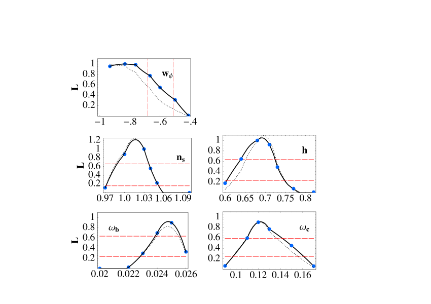
We begin by putting $\beta=0$ and assuming $V(\phi)=A\phi^{-\alpha}$. In Fig. 2 we show the likelihood for each parameter, marginalizing in turn over the others. The dotted line is for the HST prior $h=0.72\pm 0.08$. Notice that, due to the degeneracy between $w_{\phi}$ and $h$, the limits on $w_{\phi}$ are rather weak, especially if no prior is assumed. The numerical results are in Table I. Here and in the following the limits are always at the 68%(95%) c.l. while the errors are at 68% c.l.. As expected, we find results very close to those in Spergel et al. (2003). The small residual differences are probably due to the fact we use a grid instead of a Markov chain and fix $\tau$ instead of marginalizing over it.

                                          parameter WMAP WMAP+HST $w_{\phi}$ $<-0.68(-0.51)$ $<-0.73(-0.55)$ $\alpha$ $<0.94(1.92)$ $<0.74(1.64)$ $h$ 0.69${}^{+0.04}_{-0.05}$ 0.70${}^{+0.03}_{-0.05}$ $n_{s}$ 1.01$\pm$0.022 1.01$\pm$0.022 $\omega_{b}$ 0.0247$\pm$0.001 0.0247$\pm$0.0008 $\omega_{c}$ 0.12${}_{-0.01}^{+0.02}$ 0.12${}_{-0.01}^{+0.015}$ Table I. Uncoupled dark energy.

Figure 2: Likelihood functions for uncoupled dark energy models, in arbitrary units. In each panel the other parameters have been marginalized. The dotted lines are for the HST prior on the Hubble constant. The horizontal long-dashed lines are the confidence levels at 68% and 95%. The vertical long-dashed lines in the panel for $w_{\phi}$ mark the upper bounds at 68% and 95% confidence levels.

IV Coupled dark energy

In the flat conformal FRW metric $ds^{2}=-dt^{2}+a^{2}dx_{i}dx^{i}$ the scalar coupling modifies the conservation equations of dark matter and dark energy as follows:

$$\ddot{\phi}+3H\dot{\phi}+a^{2}U_{,\phi} = C\rho_{c},$$ (10)

$$\dot{\rho}_{c}+3H\rho_{c} = -C\rho_{c}\dot{\phi},$$ (11)

where $H=\dot{a}/a$. We assume that the baryons are not directly coupled to the dark energy (otherwise local gravity experiment would reveal a fifth force, see Damour et al. 1990; the radiation is automatically uncoupled with this coupling, see e.g. Amendola 1999). The dimensionless coupling

$$\beta^{2}=\frac{3C^{2}}{16\pi G},$$ (12)

can be seen as the ratio of the dark energy-dark matter interaction with respect to gravity (Damour & Nordtvedt 1993, Wetterich 1995). In Amendola (2001) we have shown that the dynamics of the system is insensitive to the sign of $\beta$, since the $\phi$MDE and the tracking phases do not depend on it. We will consider only $\beta>0.$

It is important to observe that the CMB bounds on $\beta$ depend on the existence of the $\phi$MDE. This epoch has several features that distinguish it from tracking: it is very long (from equivalence to $z\approx 10$); it depends only on the kinetic energy of the dark energy, and therefore is independent of the dark energy potential; it cannot be avoided even assuming an extremely small initial dark energy density (contrary to the tracking that may be avoided by selecting initial conditions with very low scalar field energy – the so-called “undershooting” trajectories ). Most importantly, as shown in Amendola et al. (2002), suffers less from the geometrical degeneracy that plague $w_{\phi}$, since $\Omega_{\phi}$ at decoupling is non-zero (although there still is a degeneracy $\beta-h$ in the sense that larger $h$ are compensated by larger $\beta$).

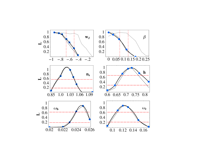
In Fig. 3 we show the likelihood for $w_{\phi},w_{e}$, marginalizing over the other parameters. We find the following constraints at 95% c.l.:

$$\alpha<2.08,\quad\beta<0.13.$$ (13)

Notice that this implies that an exponential potential (corresponding to $\alpha\to\infty$) is rejected even for $\beta\not=0$. In place of $\alpha$ and $\beta$ we can use as well as likelihood variables the equation of state during tracking and during $\phi$MDE, respectively, using Eqs. (1) and (3). Then we obtain at the 95% c.l.-

$$-1\leq w_{\phi(tracking)}<-0.49,\quad 0\leq w_{e(\phi MDE)}<0.0075.$$ (14)

This shows that the effective equation of state during $\phi$MDE, i.e. between equivalence and tracking, is close to zero (as in a pure matter dominated epoch) to less than 1%. The striking difference between the level of the two constraints in (14) indicates that the CMB is more sensitive to the dark energy coupling than to its potential, as emphasized in Amendola et al. (2003). In Fig. 4 we report the likelihood for all the parameters, contrasting the WMAP estimation with the pre-WMAP one (the limit on $\beta$ stated in Amendola et al. 2003 was slightly different because here we include more pre-WMAP data). As it can be seen, WMAP puts quite stronger limits on $w_{\phi}$ and on $\beta$. In particular, the likelihood for $w_{\phi}$ now vanishes for $w_{\phi}>-0.4$.

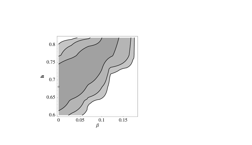
The other parameters are given in Table II. It appears that the limits on the cosmological parameters $n_{s,}\omega_{b},\omega_{c}$ are almost independent of $\beta$, while a non-zero $\beta$ favors higher $h$. The degeneracy $\beta-h$ is reported in Fig. 5.

Figure 3: Likelihood contour plots in the space $w_{\phi(tracking)}$,$w_{e(\phi MDE)}$ (or $\alpha,\beta$) marginalizing over the other parameters at the 68,95 and 99% c.l..

Figure 4: Marginalized likelihood for tracking trajectories. The solid curves are for the WMAP data, the short-dashed curves are for the HST prior, and the dotted curves in the panels for $w_{\phi}$ and $\beta$ for the pre-WMAP compilation . The horizontal long-dashed lines are the confidence levels at 68% and 95%. The vertical long-dashed lines in the panel for $w_{\phi}$ mark the upper bounds at 68% and 95% confidence levels.

Figure 5: Likelihood for $\beta,\,h$. This shows the residual degeneracy between the two parameters due to the geometric degeneracy in the angular diameter distance to last scattering.

                            parameter WMAP WMAP+HST pre-WMAP $w_{\phi}$ $<-0.67(-0.49)$ $<-0.69(-0.52)$ $<-0.50(-0.25)$ $\alpha$ $<0.99(2.08)$ $<0.90(1.84)$ $<2.0(6.0)$ $w_{e}$ $<0.0025(0.0075)$ $<0.0023(0.0075)$ $<0.0075(0.016)$ $\beta$ $<0.075(0.13)$ $<0.072(0.13)$ $<0.13(0.19)$ $h$ 0.73$\pm$ 0.05 0.73$\pm$ 0.04 >0.62(0.55) $n_{s}$ 1.019$\pm$ 0.025 1.018$\pm 0.025$ 0.97$\pm$0.03 $\omega_{b}$ 0.0247$\pm$ 0.0008 0.0250$\pm$0.0008 0.021$\pm$0.003 $\omega_{c}$ 0.123$\pm$ 0.016 0.120$\pm$ 0.016 0.12$\pm$0.04 Table II. Coupled dark energy.

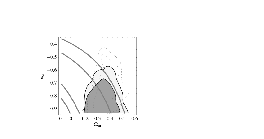
In Fig. 6 we show the contour plot of the likelihood $L(\Omega_{m},w_{\phi})$, where $\Omega_{m}=\Omega_{c}+\Omega_{b}$, marginalizing over the other parameters. We also add the confidence region from the Hubble diagram of SNIa (we used the fit C of Perlmutter et al. 1999, plus the supernova SN1997ff at $z\approx 1.75$ , Benitez et al. 2002). The product of the two likelihood functions is shown in the same figure. It turns out that $\Omega_{\phi}=0.67\pm 0.05$ and $w_{\phi}<-0.76$ (95%c.l.) (see Fig. 7). The limit on $w_{\phi}$ is very close to that obtained in Spergel et al. (2003): this shows that this bound is almost independent of the coupling $\beta.$

Figure 6: Contour plot of the likelihood function $L(\Omega_{m},w_{\phi})$. The dotted lines are for WMAP only, the thik gray lines for the supernovae Ia, and the gray regions are for the combined WMAP+SNIa (all contours at the 68% and 95% confidence levels).

Figure 7: Likelihood for $\Omega_{m}$ and $w_{\phi}$ including the constraints from supernovae Ia (marginalizing over all the other parameters, including $\beta$).

V Conclusions

CMB observations are a powerful probe to constrain the properties of dark energy. In particular, since a dark matter-dark energy interaction would obviously escape any local gravity experiment, cosmological observations like the CMB are the only way to observe such a phenomenon. Since observations require the baryons to be decoupled from dark energy (or coupled much more weakly than dark matter), the search for a non-zero coupling $\beta$ is also a test of the equivalence principle. We found that current CMB data are capable to put an interesting upper bound to the present dark energy equation of state (all limits to 95% c.l.)

$$w_{\phi}<-0.49,$$ (15)

which becomes $<-0.76$ taking into account SNIa data (let us remember that in our tracking models $w_{\phi}$ is confined to be $\geq-1$) and to the total dark energy density,

$$\Omega_{\phi}=0.67\pm 0.05.$$ (16)

For the dark matter - dark energy coupling we obtain:

$$|\beta|<0.13,$$ (17)

regardless of the potential (within the tracking class we considered), corresponding to a past equation of state $0\leq w_{e(\phi MDE)}<0.0075$. This implies that the scalar gravity is at least $1/\beta^{2}\approx 60$ times weaker than ordinary tensor gravity. As shown in Amendola (1999), the limit on $\beta$ can be restated as a limit on the constant $\xi$ of the non-minimally coupled gravity, $\xi<0.01$. We have shown in Amendola et al. (2003) that an experiment like the Planck mission can lower the upper bound to $\beta$ to 0.05. a limit comparable to the constraint that local gravity experiments impose on the scalar gravity coupling to baryons, $\beta_{baryons}^{2}<10^{-3}$ (see e.g. Hagiwara et al. 2002).

Appendix

Suppose we have the binned observational spectra $C^{\prime}_{\ell,d}=(1+b_{e})C_{\ell,d}$ and the binned theoretical spectra $C^{\prime}_{\ell,t}=\hat{b}_{t}C_{\ell,t}$ from a given experiment labelled $e$, where $b_{e}$ is a calibration factor which is assumed to be distributed as a Gaussian with zero mean and variance $\sigma_{e}$ and $\hat{b}_{t}$ is the overall theoretical normalization, which is uniformly distributed in $(0,\infty)$. Let $N_{e}$ be the correlation matrix for the $e$-th experiment and

$$N^{\prime}_{e}=(C_{d}^{T}C_{d})^{-1}N_{e}$$ (18)

the approximated correlation function for the lognormal variables $Z\equiv\log C$ (here and in the following we suppress for clarity the indexes $\ell\ell^{\prime}$ of the correlation matrices and the index $\ell$ from the vectors $Z,C_{t},C_{d}$) . If the assumed likelihood is log-normal then we can integrate out $b_{e}$ as follows

$$L_{e} = \int\prod_{e}db_{e}e^{-\frac{1}{2}\left(\frac{b_{e}}{\sigma_{e}}\right)^{2}}\times$$ (20)

$$\exp\left\{-\frac{1}{2}\sum_{e}\left[Z^{\prime}_{t}-b_{e}-Z_{d}\right]N_{e}^{,-1}\left[Z^{\prime}_{t}-b_{e}-Z_{d}\right]\right\}=\int db_{t}\prod_{e}L_{e}$$

where $Z^{\prime}_{t}=\log\hat{b}_{t}C_{t}$ and $b_{e}\approx\log(b_{e}+1),Z_{d}=\log C_{d}$ (for small $b_{e}$) so that

$$L_{e}=\exp\left[-\frac{1}{2}\left(Z^{\prime}_{t}-Z_{d}\right)W_{e}^{-1}\left(Z^{\prime}_{t}-Z_{d}\right)\right]$$ (21)

where

$$W_{e}=(C_{d}^{T}C_{d})^{-1}N_{e}+\sigma_{e}^{2}I^{T}I$$

where $I=(1,1,1,...,n_{e})$, $n_{e}$ being the number of datapoints in the $e$-th experiment. Note in fact that (Woodbury formula, see e.g. Melchiorri et al. 2002)

$$(N+XX^{T})=N^{-1}-\left[N^{-1}X(1+X^{T}N^{-1}X)^{-1}X^{T}N^{-1}\right]$$

which gives the above if $X=\sigma_{e}I$.

Suppose now the experimental spectra are distorted by a further $\ell$-dependent factor $(1+w_{e}A_{\ell})$ due to the uncertainty on the beam angular size, where $w$ is a random variable distributed as a Gaussian with variance $\sigma_{w,e}$ and $A_{\ell}$ is a constant vector determined by the experiment. Then each likelihood $L_{e}$ should be further integrated as follows

$$L^{\prime}_{e} = \int dw_{e}L_{e}=\int dw_{e}e^{-\frac{1}{2}\left(\frac{w_{e}}{\sigma_{w,e}}\right)^{2}}\times$$ (22)

$$= \exp\left[-\frac{1}{2}\left(w_{e}A+Z^{\prime}_{t}-Z_{d}\right)W_{e}^{-1}\left(w_{e}A+Z^{\prime}_{t}-Z_{d}\right)\right]$$ (23)

where, on applying again the Woodbury formula,

$$L^{\prime}_{e}=\exp\left[-\frac{1}{2}\left(Z^{\prime}_{t}-Z_{d}\right)M_{e}^{-1}\left(Z^{\prime}_{t}-Z_{d}\right)\right]$$ (25)

where

$$M_{e}=(C^{T}C)^{-1}N_{e}+\sigma_{e}^{2}I^{T}I+\sigma_{w,e}^{2}A^{T}A$$ (26)

In the case of a Gaussian beam of angular size $\theta_{0}$ the spectrum is multiplied by a factor $e^{\ell^{2}\theta_{0}^{2}}$. It can be seen then that a small misestimate $\theta$ (assumed to be distributed as a Gaussian variable with variance $\sigma_{\theta}$ ) of the beam size induces a correction on the spectrum at the $\ell-th$ bin by a factor $[1+\ell^{2}(\theta_{0}^{2}-\theta^{2})]=1+w\ell^{2}$, where the random variable $w\approx 2\theta_{0}(\theta_{0}-\theta)$ is also Gaussian and has uncertainty $\sigma_{w}=2\theta_{0}\sigma_{\theta}$. The vector $A_{\ell}$ can be approximated then as $\ell^{2}$.

Finally, we integrate over $b_{t}=\log\hat{b}_{t}$. Then we have $Z_{t}=b_{t}+Z^{\prime}_{t}$ and

$$L=\int db_{t}\prod_{e}L^{\prime}_{e}(b_{t}) = \int_{-\infty}^{\infty}db_{t}\exp\left[-\frac{1}{2}\sum_{e}\left(b_{t}+Z_{t}-Z_{d}\right)M_{e}^{-1}\left(b_{t}+Z_{t}-Z_{d}\right)\right]$$ (27)

$$= \exp\left[-\frac{1}{2}\left(\gamma-\frac{\beta^{2}}{\alpha}\right)\right]$$ (28)

where

$$\alpha = \sum_{e}I^{T}M_{e}^{-1}I$$

$$\beta = \sum_{e}I^{T}M_{e}^{-1}(Z_{t}-Z_{d})$$

$$\gamma = \sum_{e}(Z_{t}-Z_{d})^{T}M_{e}^{-1}(Z_{t}-Z_{d})$$

which is the formula we use in this paper for the pre-WMAP data.

References

- (1) Amendola L., Phys. Rev. D60, 043501, (1999), astro-ph/9904120
- (2) Amendola L. & D. Tocchini-Valentini, (2001) Phys. Rev. D64, 043509, astro-ph/0011243,
- (3) Amendola L., Phys. Rev. D62, 043511 (2000), astro-ph/9908440;
- (4) Amendola L., Phys. Rev. Lett., 86, 196 (2001), astro-ph/0006300
- (5) Amendola L. & D. Tocchini-Valentini (2002), Phys. Rev. D66, 043528 astro-ph/0111535
- (6) Amendola L., C. Quercellini, D. Tocchini-Valentini & A. Pasqui, ApJ L., inpress
- (7) Baccigalupi C., Perrotta F. & Matarrese S., Phys. Rev. D61, 023507 (2000)
- (8) Baccigalupi C., A. Balbi, S. Matarrese, F. Perrotta, N. Vittorio,(2001) astro-ph/0109097 Phys.Rev.D65:063520,2002
- (9) Bean R. & Magueijo J., Phys. Rev. B517 (2000), 177-183
- (10) Bennett C.L. et al. Ap. J. 464, L1 (1996)
- (11) Benoit et al. [Archeops collaboration] A&A, submitted (2002)
- (12) Billyard A.P. & Coley A.A., Phys. Rev. D60 (2000) 083503
- (13) Caldwell R.R., Doran M., Muller C., Schafer G., Wetterich C., astro-ph/0302505
- (14) Caldwell R.R., Dave R. & Steinhardt P.J. (1998), Phys. Rev. Lett. 80, 1582
- (15) Chen X. & Kamionkowski M., Phys. Rev. D60, 104036, astro-ph/9905368
- (16) Chiba T., Phys. Rev. D60, 083508 (1999)
- (17) Chimento L.P., A. S. Jakubi & D. Pavon, Phys. Rev. D62, 063508 (2000), astro-ph/0005070;
- (18) Corasaniti P.S. & E. Copeland, astro-ph/0107378, Phys.Rev.D65, 043004,2002
- (19) Damour T. & Nordtvedt K., Phys. Rev. Lett. 70, 2217 (1993)
- (20) Damour T., G. W. Gibbons and C. Gundlach, Phys. Rev. Lett., 64, 123, (1990)
- (21) Doran M., Lilley M., Wetterich C., (2001) astro-ph/0105457, Phys.Lett.B528:175-180,2002
- (22) Esposito-Farese G. & D. Polarsky, Phys. Rev. D63, 063504 (2001) gr-qc/0009034
- (23) Ferreira P.G. & Joyce M., Phys. Rev. D58, 023503 (1997) astro-ph/9711102
- (24) Frieman J., Hill C.T., Stebbins A. & I. Waga, Phys. Rev. Lett. 75, 2077 (1995)
- (25) Freedman W. et al. Ap.J. 553 (2001) 47.
- (26) Gasperini M., F. Piazza and G. Veneziano, (2001) gr-qc/0108016 Phys.Rev.D65, 023508,2002
- (27) Hagiwara K. et al., Phys. Rev. D66 010001-1 (2002), available at pdg.lbl.gov
- (28) Halverson N. W. et al., (2001) Ap.J. 568, 38 (2002), astro-ph/0104489.
- (29) Hinshaw G. et al. [WMAP collaboration] Ap.J. submitted (2003)
- (30) Holden D.J. & Wands D., Phys. Rev. D61 (2000) 043506
- (31) Lee A.T. et al., Ap.J. 561, L1 (2001) astro-ph/0104459.
- (32) Melchiorri A., Mersini L., Odman C., and Trodden M., astro-ph/0211522 (2002)
- (33) Netterfield C. B. et al., (2001) Ap.J. 571, 604 (2002) astro-ph/0104460.
- (34) Pearson T.J. et al. Ap.J. astro-ph/0205388 (2002)
- (35) Perlmutter S. et al. (1999) Ap.J., 517, 565
- (36) Pietroni M., (2002) hep-ph/0203085
- (37) Ratra B. & P.J.E. Peebles, Phys. Rev. D37, 3406 (1988)
- (38) Riess A.G. et al. A.J., 116, 1009 (1998)
- (39) Scott P.F. et al. astro-ph/0205380 (2002)
- (40) Sen A.A. & S. Sen, MPLA, 16, 1303 (2001), gr-qc/0103098;
- (41) Seljak U. and M. Zaldarriaga, Ap.J., 469, 437 (1996).
- (42) Spergel D.N. et al. [WMAP collaboration], Ap.J. submitted (2003)
- (43) Steinhardt P.J., L. Wang, I. Zlatev, Phys.Rev. D59 (1999) 123504
- (44) Uzan J.P., Phys. Rev. D59, 123510 (1999)
- (45) Verde L. et al. [WMAP collaboration], Ap.J. submitted (2003)
- (46) Wang X., Tegmark M., and Zaldarriaga M., astro-ph/0105091, Phys. Rev. D65, 123001 (2002)
- (47) Wetterich C.. (1988) Nucl. Phys. B., 302, 668;
- (48) Wetterich C., (1995) A& A, 301, 321