Quintessence and the Curvature of the Universe after WMAP

Abstract

We study quintessence models with a constant (effective) equation of state. It is investigated whether such quintessence models are consistent with a negative spatial curvature of the Universe with respect to the anisotropy of the cosmic microwave background radiation measured by the WMAP mission. If the reionization is negligibly small, it is found that such models with negative curvature are admissible due to a geometrical degeneracy. However, a very high optical depth $\tau$ to the surface of last scattering, as indicated by the polarization measurements of WMAP, would rule out such models.

Received (received date)Revised (revised date)

1 Introduction

During the last decade, observational cosmology has made enormous progress. In particular, the spectacular discovery in 1992 of the temperature fluctuations of the cosmic microwave background (CMB) radiation by COBE [1] has provided important clues about the early Universe and its time evolution. Although the measured anisotropy of the CMB (being of the order of $10^{-5}$) is quite small, it sheds important light on several basic physical mechanisms (see Refs. [2, 3, 4] for reviews summarizing the last stand before WMAP). The first findings of NASA’s explorer mission “Wilkinson Microwave Anisotropy Probe” (WMAP) [5] has tremendously increased our knowledge of the temperature fluctuations of the CMB, since WMAP has measured the anisotropy of the CMB radiation over the full sky with high accuracy. It is the purpose of this paper to test our theoretical understanding of physical cosmology by making use of the high quality of the WMAP data.

One of the most important results of the cosmological observations made during the last few years has been that all tests of cosmology probing the nature of matter resp. energy in the Universe suggest that our Universe is at the present epoch not dominated by matter but rather by a mysterious energy with negative pressure (see Ref. [2] for a recent review of the state of the Universe). There are essentially two models to explain this new energy component which nowadays is called dark energy. One possibility is to identify the dark energy with Einstein’s cosmological constant $\Lambda$ with a corresponding energy density $\varepsilon_{\Lambda}=\Lambda c^{4}/(8\pi G)$ and negative pressure $p_{\Lambda}=-\varepsilon_{\Lambda}$, assuming a positive cosmological constant. An alternative explanation is quintessence [6, 7, 8, 9, 10], where the dark energy is identified with the energy density $\varepsilon_{\phi}$ arising from a time-evolving scalar (quintessence) field $\phi$ (see Refs. [11, 12] for recent reviews). An important cosmological parameter is the equation of state of the dark energy component, which in the case of quintessence is given by $w_{\phi}:=p_{\phi}/\varepsilon_{\phi}$, where $p_{\phi}$ denotes the associated pressure. Quintessence models can be considered as generalizations of the cosmological constant and include the latter as the special case $w_{\phi}=\hbox{const.}=-1$. In general, the equation of state $w_{\phi}$ can be a function of redshift. In our following analysis of the WMAP data, we shall assume, however, $w_{\phi}=\hbox{const.}\geq-1$. These models have the property that their quintessence component is negligible at early times such as the recombination epoch. (There are also models with a time-dependent $w_{\phi}$ which lead to “early quintessence” models [13], which are, however, not discussed in this paper.) First of all, a constant equation of state for the dark energy component represents an obvious and also the simplest generalization of the other known energy components of the Universe which have the constant values $w_{\hbox{\scriptsize r}}=1/3$ (for radiation) and $w_{\hbox{\scriptsize m}}=0$ (for matter). Secondly, as discussed e. g. in Refs. [14, 15, 16, 17, 18], there is an inherent theoretical limitation to determine the time variation of the equation of state of the dark energy component. For example, the luminosity distance $d_{L}$ and the angular-diameter distance $d_{A}$ depend on $w_{\phi}$ through a multiple-integral relation that smears out detailed information about the redshift dependence of $w_{\phi}(z)$ (see Eqs. (5) and (6) below).

One of the most fundamental cosmological parameters is the curvature of the Universe. Many cosmologists seem to accept as established that the Universe is flat corresponding to $k=0$ and $\Omega_{\hbox{\scriptsize tot}}:=\varepsilon_{\hbox{\scriptsize tot}}/\varepsilon_{\hbox{\scriptsize crit}}=1$. Contrary to that opinion, we shall demonstrate that the WMAP data are consistent with certain quintessence models possessing a constant equation of state in a hyperbolic universe, i. e. with negative spatial curvature, $k=-1$, corresponding to $\Omega_{\hbox{\scriptsize tot}}<1$, provided that the optical depth $\tau$ is negligibly small. Our result is the consequence of the crucial observation that there exists a degeneracy in the space of the relevant cosmological parameters $(\Omega_{\hbox{\scriptsize tot}},\Omega_{\phi},w_{\phi})$, where $\Omega_{\phi}:=\varepsilon_{\phi}/\varepsilon_{\hbox{\scriptsize crit}}$ is the ratio of the quintessence energy density to the critical density.

2 Quintessence models

Our background model is the standard cosmological model based on a Friedmann–Lemaître universe with Robertson-Walker metric. Then the Friedmann equation reads $(a^{\prime}:=da/d\eta,c=1)$

$$H^{2}:=\left(\frac{a^{\prime}}{a^{2}}\right)^{2}\;=\;\frac{8\pi G}{3}\varepsilon_{\hbox{\scriptsize tot}}-\frac{k}{a^{2}}\hskip 10.0pt,$$ (1)

where $a(\eta)$ is the cosmic scale factor as a function of conformal time $\eta$ and $H=H(\eta)$ is the Hubble parameter. The last term in Eq. (1) is the curvature term. Furthermore, $\varepsilon_{\hbox{\scriptsize tot}}:=\varepsilon_{\hbox{\scriptsize r}}+\varepsilon_{\hbox{\scriptsize m}}+\varepsilon_{\phi}$, where $\varepsilon_{\hbox{\scriptsize r}}$ denotes the energy density of “radiation”, i. e. of the relativistic components according to photons and three massless neutrinos; $\varepsilon_{\hbox{\scriptsize m}}=\varepsilon_{\hbox{\scriptsize b}}+\varepsilon_{\hbox{\scriptsize cdm}}$ is the energy density of non-relativistic “matter” consisting of baryonic matter, $\varepsilon_{\hbox{\scriptsize b}}$, and cold dark matter, $\varepsilon_{\hbox{\scriptsize cdm}}$, and $\varepsilon_{\phi}$ is the energy density of the dark energy due to the quintessence field $\phi$.

In quintessence models, the energy density $\varepsilon_{\phi}(\eta)$ and the pressure $p_{\phi}(\eta)$ of the dark energy are determined by the quintessence potential $V(\phi)$

$$\varepsilon_{\phi}\;=\;\frac{1}{2a^{2}}\,{\phi^{\prime}}^{2}+V(\phi)\hskip 10.0pt,\hskip 10.0ptp_{\phi}\;=\;\frac{1}{2a^{2}}\,{\phi^{\prime}}^{2}-V(\phi)\hskip 10.0pt,$$ (2)

or equivalently by the equation of state $w_{\phi}=\frac{p_{\phi}}{\varepsilon_{\phi}}$. The equation of motion of the real, scalar field $\phi(\eta)$ is

$$\phi^{\prime\prime}\,+\,2\frac{a^{\prime}}{a}\phi^{\prime}\,+\,a^{2}\frac{\partial V(\phi)}{\partial\phi}\;=\;0\hskip 10.0pt,$$ (3)

where it is assumed that $\phi$ couples to matter only through gravitation. The various energy densities are constrained by the continuity equation

$$\varepsilon_{\hbox{\scriptsize x}}^{\prime}\,+\,3(1+w_{\hbox{\scriptsize x}})\,\frac{a^{\prime}}{a}\,\varepsilon_{\hbox{\scriptsize x}}\;=\;0\hskip 10.0pt,$$ (4)

with the constant equation of state $w_{\hbox{\scriptsize r}}=\frac{1}{3}$, $w_{\hbox{\scriptsize m}}=0$ for $\hbox{x}=\hbox{r},\hbox{m}$, respectively, and $w_{\phi}(\eta)$ for $\hbox{x}=\phi$. It is worthwhile to remark that the quintessence field $\phi$ may be regarded as a real physical field, or simply as a device for modeling more general cosmic fluids with negative pressure. Since $w_{\phi}$ is assumed to be constant, the potential $V(\phi)$ is uniquely determined as shown in Refs. [10, 18]. However, in solving numerically the coupled Eqs. (1)-(4) no knowledge of the potential $V(\phi)$ is required.

3 Comparison with the WMAP data

In our comparison with the WMAP data, we make the following assumptions [2]. The Hubble constant $H_{0}=h\times 100\hbox{ km s}^{-1}\hbox{Mpc}^{-1}$ is set to $h=0.70$, and the baryonic density parameter $\Omega_{\hbox{\scriptsize b}}=0.05$ (i. e. $\Omega_{\hbox{\scriptsize b}}h^{2}=0.0245$) is chosen in agreement with the current Big-Bang nucleosynthesis constraints. Furthermore, the initial curvature perturbation is assumed to be scale-invariant $(n_{S}=1)$ which is suggested by inflationary models. We have also studied models having a spectral index $n_{S}=0.95$, but the WMAP data alone, i. e. not taking into account large-scale structure data, prefer models having $n_{S}=1$. (We do not consider a $k$-dependent spectral index $n_{S}$ in this paper.) In addition, we have varied the Hubble constant over the range $h=0.64\dots 0.72$, but the best models for a fixed curvature all prefer a value close to $h=0.70$. The optical depth $\tau$ to the surface of last scattering is in this Section assumed to be negligibly small. In the next Section, we use the surprisingly high value of $\tau$ found by WMAP[19]. The CMB anisotropy of the quintessence models is computed using the publicly available CAMB code by Antony Lewis and Antony Challinor together with the quintessence module for $w_{\phi}=\hbox{const.}$ models. The angular power spectrum $\delta T_{l}^{2}=l(l+1)C_{l}/2\pi$ is compared with the one obtained by WMAP [20] which comprises 899 data points. The amplitude of the initial curvature perturbation is determined such that the value of $\chi_{\hbox{\scriptsize eff}}^{2}$ is minimized. The values of $\chi_{\hbox{\scriptsize eff}}^{2}$ are obtained by using the FORTRAN code (provided by the WMAP team [21]) which, given a theoretical CMB power spectrum, computes the likelihood of that model fit to the WMAP data.

Figure 1: The $\chi^{2}$ values are shown in dependence on $w_{\phi}$ and $\Omega_{\phi}$ for $\Omega_{\hbox{\scriptsize tot}}=0.85$, $h=0.70$, $\tau=0.0$ and $n_{s}=1.0$ using the WMAP data. The curves with $\chi_{\hbox{\scriptsize eff}}^{2}=1020$, 1100, 1200 and 1300 are indicated. The minimum $\chi^{2}_{\hbox{\scriptsize min}}=1016$ occurs at $\Omega_{\phi}=0.54$, $w_{\phi}=-0.26$.

Figure 2: The same as in Fig. 1 for $\Omega_{\hbox{\scriptsize tot}}=0.9$. The curves with $\chi_{\hbox{\scriptsize eff}}^{2}=990$, 1000, 1100, 1200 and 1300 are indicated. The minimum $\chi^{2}_{\hbox{\scriptsize min}}=985$ occurs at $\Omega_{\phi}=0.59$, $w_{\phi}=-0.36$.

Figure 3: The same as in Fig. 1 for $\Omega_{\hbox{\scriptsize tot}}=0.95$. The curves with $\chi_{\hbox{\scriptsize eff}}^{2}=980$, 1000, 1100, 1200 and 1300 are indicated. The minimum $\chi^{2}_{\hbox{\scriptsize min}}=975$ occurs at $\Omega_{\phi}=0.61$, $w_{\phi}=-0.58$.

Figure 4: The same as in Fig. 1 for $\Omega_{\hbox{\scriptsize tot}}=1.0$. The curves with $\chi_{\hbox{\scriptsize eff}}^{2}=980$, 1000, 1100, 1200 and 1300 are indicated. The minimum $\chi^{2}_{\hbox{\scriptsize min}}=978$ occurs at $\Omega_{\phi}=0.68$, $w_{\phi}=-1.0$.

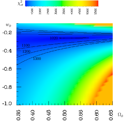
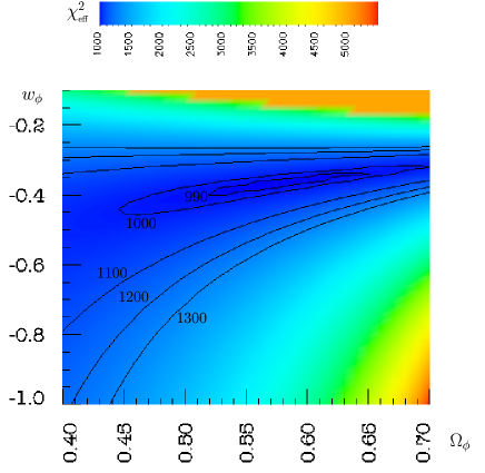
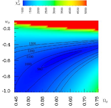
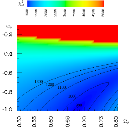
Figures 1 to 4 present the values of $\chi_{\hbox{\scriptsize eff}}^{2}$ for the four cases $\Omega_{\hbox{\scriptsize tot}}=0.85,0.9,0.95$ and $1.0$, respectively, in dependence on $w_{\phi}$ and $\Omega_{\phi}$. Since $\Omega_{\hbox{\scriptsize tot}}$ is held fixed, the matter density $\Omega_{\hbox{\scriptsize m}}:=\Omega_{\hbox{\scriptsize b}}+\Omega_{\hbox{\scriptsize cdm}}$ is given by $\Omega_{\hbox{\scriptsize m}}=\Omega_{\hbox{\scriptsize tot}}-\Omega_{\phi}$ neglecting the small radiation contribution. One observes that a decreasing $\Omega_{\hbox{\scriptsize tot}}$ demands an increasing $w_{\phi}$, i. e. a less negative value; from $\Omega_{\hbox{\scriptsize tot}}=0.85$ to $\Omega_{\hbox{\scriptsize tot}}=1.0$ the equation of state changes from $w_{\phi}=-0.26$ to $w_{\phi}=-1.0$. Among the models considered, the best fit to the WMAP data is obtained for the model with $\Omega_{\hbox{\scriptsize tot}}=0.95$, $\Omega_{\phi}=0.61$ and $w_{\phi}=-0.58$ belonging to the minimum at $\chi_{\hbox{\scriptsize eff}}^{2}=975$, see Figure 3. The corresponding angular power spectrum $\delta T_{l}^{2}$ is shown as a full curve in Figures 5 and 6 and compared with the WMAP measurements. The model with $\Omega_{\hbox{\scriptsize tot}}=0.90$, $\Omega_{\phi}=0.59$ and $w_{\phi}=-0.36$ is almost of the same quality and belongs to the minimum at $\chi_{\hbox{\scriptsize eff}}^{2}=985$ (see Figure 2) compared to the 899 data points of WMAP. The corresponding $\delta T_{l}^{2}$ is shown as dashed curve in Figures 5 and 6. Assuming a flat universe, $\Omega_{\hbox{\scriptsize tot}}=1.0$, one obtains a broad, but extremely flat $\chi_{\hbox{\scriptsize eff}}^{2}$-valley as shown in Figure 4. The best flat model is obtained for $\Omega_{\phi}=0.68$ and $w_{\phi}=-1.0$ and is plotted as dotted curve in Figures 5 and 6. This model possesses a $\chi_{\hbox{\scriptsize eff}}^{2}$-value of $\chi_{\hbox{\scriptsize eff}}^{2}=978$. It is worth noting that the $\chi_{\hbox{\scriptsize eff}}^{2}$-valleys get increasingly narrower with a horizontal alignment in Figures 1-4 with decreasing $\Omega_{\hbox{\scriptsize tot}}$ and thus allow only a small variation in $w_{\phi}$. In the case $\Omega_{\hbox{\scriptsize tot}}=0.85$, one observes the most confined valley, see Figure 1, where the best model with $\Omega_{\phi}=0.54$ and $w_{\phi}=-0.26$ has $\chi_{\hbox{\scriptsize eff}}^{2}=1016$. It is seen in Figures 5 and 6 that the best models corresponding to the cases $\Omega_{\hbox{\scriptsize tot}}=0.85,0.9,0.95$ and $1.0$, respectively, are nearly degenerate with respect to their angular power spectrum $\delta T_{l}^{2}$. The main difference occurs for small values of $l$ where the integrated Sachs-Wolfe effect yields with decreasing $\Omega_{\hbox{\scriptsize tot}}$ and increasing $w_{\phi}$ a larger contribution. However, this discrepancy scarcely influences the value of $\chi_{\hbox{\scriptsize eff}}^{2}$ due to the cosmic variance. In contrast, the position of the acoustic peaks and their relative heights are nearly indistinguishable. Even with the high accuracy of the WMAP data, one can hardly discriminate between these models.

Figure 5: The angular power spectrum $\delta T_{l}^{2}$ is presented for the four best models for the cases $\Omega_{\hbox{\scriptsize tot}}=0.85,0.9,0.95$ and $\Omega_{\hbox{\scriptsize tot}}=1.0$ and compared with the WMAP[5] data. The model fits are determined by the minima of $\chi_{\hbox{\scriptsize eff}}^{2}$ shown in Figures 1 to 4.

Figure 6: The same angular power spectra $\delta T_{l}^{2}$ as in Figure 5 are presented in a linear $l$-scale.

Figure 7: The position $l_{1}$ of the first acoustic peak is computed in dependence on $w_{\phi}$ and $\Omega_{\hbox{\scriptsize c}}=1-\Omega_{\hbox{\scriptsize tot}}$ for $\Omega_{\hbox{\scriptsize b}}=0.05$ and $\Omega_{\hbox{\scriptsize cdm}}=0.27$. The white curves indicate the peak position for $l_{1}=180,200,240$ and 260. The black curve belongs to $l_{1}=220$.

The identical position of the peaks is mainly due to a geometrical degeneracy [22, 18] which arises through the angular-diameter distance $d_{A}$ to the surface of last scattering which has to be computed by $(\Omega_{\hbox{\scriptsize c}}:=1-\Omega_{\hbox{\scriptsize tot}})$

$$d_{A}\;=\;\frac{1}{H_{0}\sqrt{|\Omega_{\hbox{\scriptsize c}}|}(1+z_{\hbox{\scriptsize sls}})}\,S_{k}\left(H_{0}\sqrt{|\Omega_{\hbox{\scriptsize c}}|}\int_{1}^{1+z_{\hbox{\scriptsize sls}}}\frac{dx}{H(x)}\,\right)\hskip 5.0pt,$$ (5)

where $S_{k}(y)$ denotes $\sinh y$, $y$, $\sin y$ for $k=-1,0,+1$, respectively. The Hubble parameter $H(x)$, $x=z+1$, is given by

$$\left(\frac{H(x)}{H_{0}}\right)^{2}=\Omega_{\hbox{\scriptsize r}}x^{4}+\Omega_{\hbox{\scriptsize m}}x^{3}-k\Omega_{\hbox{\scriptsize c}}x^{2}+\Omega_{\phi}e^{3\int_{1}^{x}(1+w_{\phi}(x^{\prime}))\frac{dx^{\prime}}{x^{\prime}}}\hskip 2.0pt.$$ (6)

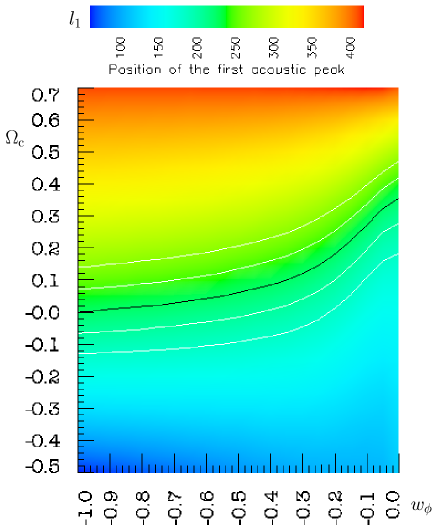
The degeneracy due to $d_{A}$ has been discussed by several authors [22, 23, 16, 17, 18, 24, 25], in particular in the neighborhood of a flat universe and for $w_{\phi}$ near $-1$. One emphasis has been on the dependence of the position $l_{1}$ of the first acoustic peak in the angular power spectrum of the CMB anisotropy on the various cosmological parameters. As a result, it has been concluded that, although there is a degeneracy with respect to $\Omega_{\phi}$ and $w_{\phi}$, the position of the first peak is well suited for a determination of the curvature of the Universe. Analyzing the CMB anisotropy and other cosmological observations has led many cosmologists to accept that the Universe is flat in accordance with the inflationary scenarios. However, admitting also quintessence models with $w_{\phi}>-1$ changes this simple picture, since there exists now a degeneracy in the $(\Omega_{\hbox{\scriptsize tot}},\Omega_{\phi},w_{\phi})$-space. In Ref. [18] the dependence of $d_{A}$ on the curvature and on $w_{\phi}$ has been investigated using the CMB data before WMAP and it has been shown that there exists a family of models with different curvature having all the same $d_{A}$. In Figure 7 we show the position $l_{1}$ of the first acoustic peak (computed using CAMB) for a large class of models sharing the cosmological parameters $\Omega_{\hbox{\scriptsize cdm}}=0.27$, $h=0.70$, $\tau=0.0$ and $n_{S}=1.0$. The WMAP data confines the position of the first peak close to $l_{1}\simeq 220$ [20]. The models possessing $l_{1}=220$ are connected by the black curve in Figure 7. It is worthwhile to note that the curve for $l_{1}=220$ allows flat models as well as models with negative curvature, but not with positive curvature. Using the WMAP data, the best models, shown in Figures 5 and 6, belong to models lying close to this black curve. The existence of this family in the parameter space $(\Omega_{\hbox{\scriptsize tot}},\Omega_{\phi},w_{\phi})$ of equal values of $l_{1}$ is mainly due to the degeneracy in $d_{A}$. Under the assumption that the reionization has no significant influence on the CMB anisotropy, we conclude that this geometrical degeneracy allows our Universe to possess negative spatial curvature compatible with the new WMAP data.

4 Polarization and the influence of early reionization

Figure 8: Panel a) shows the reionization suppression ${\cal R}:=C_{l}(\tau=0.15)/C_{l}(\tau=0.0)$ for the two “best” models for $\Omega_{\hbox{\scriptsize tot}}=1.0$ (solid curve) and $\Omega_{\hbox{\scriptsize tot}}=0.9$ (dashed curve), if the optical depth $\tau$ is increased from $\tau=0.0$ to $\tau=0.15$. Panel b) shows $\delta T_{l}^{2}$ for these two cases with $\tau=0.0$ (solid curves) and $\tau=0.15$ (dashed curves). The two upper curves at low values of $l$ belong to the case with $\Omega_{\hbox{\scriptsize tot}}=0.9$.

WMAP has also obtained data for the correlation of the polarization with the temperature variations [19]. This data requires an unexpected high optical depth $\tau$ to the surface of last scattering of $\tau=0.17\pm 0.04$ [19] and $\tau=0.17\pm 0.07$ [26]. This early reionization erases some of the primary anisotropy below the corresponding horizon (reionization damping) [27] which roughly corresponds to $l\simeq 10$ for the considered models. Thus the angular power spectrum is only slightly altered below $l\simeq 10$ as can be seen in Figure 8a) in the case of our two best models for $\Omega_{\hbox{\scriptsize tot}}=1.0$ and $\Omega_{\hbox{\scriptsize tot}}=0.9$, respectively. For $l\gtrsim 100$ the reionization damping is almost independent of $l$ and, thus, does not alter the peak structure. The erased power for $l\gtrsim 10$, i. e.  the reduced peak height (proportional to $e^{-2\tau}$), is compensated by increasing the initial perturbation amplitude in order to obtain a first peak of the right amplitude. As a consequence the multipoles below $l\simeq 10$ are increased in comparison with models possessing negligible reionization as shown in Figure 8b). A close inspection of Figure 5 reveals that our models with negative curvature already possess a bit too much power for small values of $l$. These models have been computed with negligible optical depth $\tau=0$ to the surface of last scattering. Thus increasing the optical depth $\tau$ increases the power for small values of $l$ so severely that the models get such high values of $\chi_{\hbox{\scriptsize eff}}^{2}$ that they are very unlikely.

Figure 9: The cross power spectra $(l+1)C_{l}^{\hbox{\scriptsize{TE}}}/(2\pi)$ are presented for the four best models for the cases $\Omega_{\hbox{\scriptsize tot}}=0.85,0.9,0.95$ and $\Omega_{\hbox{\scriptsize tot}}=1.0$ and compared with the WMAP[19] data. The model fits are determined by the minima of $\chi_{\hbox{\scriptsize eff}}^{2}$ shown in Figures 1 to 4.

Figure 10: The same cross power spectra $(l+1)C_{l}^{\hbox{\scriptsize{TE}}}/(2\pi)$ as in Figure 9 are presented in a logarithmic $l$-scale. The large rise of the measured power for $l\lesssim 10$ is an indication for a very early reionization.

Before returning to the high optical depth $\tau$, we would like to show in Figure 9 that our models describe the TE-correlation $C_{l}^{\hbox{\scriptsize{TE}}}$ of the polarization with the temperature variations for $l\gtrsim 6$ very well. (Note that there are no free parameters, since all parameters have already been fixed by the TT power spectrum.) Here the data obtained by WMAP [19] are shown in comparison with the four models discussed above ignoring the reionization. One observes that the oscillations are very well described by all four models, and that the models are again degenerated. In order to emphasize the oscillations, we have chosen a scale in Figure 9 which does not show some data points below $l\lesssim 5$. In Figure 10 we show the same data as in Figure 9 using a logarithmic scale. One observes that the models do not describe the high observed values below $l\lesssim 6$. To describe these high values, a large optical depth $\tau$ is required.

Figure 11: The cross power spectra $(l+1)C_{l}^{\hbox{\scriptsize{TE}}}/(2\pi)$ are shown for three models with $\tau=0.15$, $\Omega_{\hbox{\scriptsize b}}=0.05$ and $\Omega_{\hbox{\scriptsize cdm}}=0.27$. The solid curve belongs to a flat model with $\Omega_{\hbox{\scriptsize tot}}=1.0$, $\Omega_{\phi}=0.68$ and $w_{\phi}=-1.0$, the dashed curve to a model which differs from the preceding one only in the increased $w_{\phi}=-0.5$, and the dotted curve belongs to a model where $\Omega_{\phi}$ is reduced to $\Omega_{\phi}=0.58$, such that the model has $\Omega_{\hbox{\scriptsize tot}}=0.9$.

Figure 11 shows three models with a large optical depth $\tau=0.15$ and with $\Omega_{\hbox{\scriptsize b}}=0.05$ and $\Omega_{\hbox{\scriptsize cdm}}=0.27$. The model belonging to the solid curve is a flat model, i. e. having $\Omega_{\phi}=0.68$, with a cosmological constant $w_{\phi}=-1.0$. This model shows the required increase for very small values of $l$. Replacing the cosmological constant by a quintessence component with $w_{\phi}=-0.5$ reduces the power as shown by the dashed curve in Figure 11. Thus quintessence models require an even higher value of $\tau$ in order to obtain the same high level of TE-correlation for low values of $l$. The same behavior is observed if one changes instead of the equation of state $w_{\phi}$ the curvature, i. e. $\Omega_{\hbox{\scriptsize tot}}$. The dotted curve belongs to a model which differs from the one corresponding to the solid curve by a reduced $\Omega_{\phi}=0.58$, i. e. a model with $\Omega_{\hbox{\scriptsize tot}}=0.9$. This curve reveals suppressed power at low values of $l$ in comparison to the flat case. Models with negative curvature $\Omega_{\hbox{\scriptsize tot}}<1$ require also $w_{\phi}>-1$ in order to obtain for the first acoustic peak a position around $l\simeq 220$, as shown in Figure 7. However, as we have just seen, both ingredients, the increased $w_{\phi}$ as well as the negative curvature, reduce the level of TE-correlation at low values of $l$. To describe the observed TE-correlation, extremely high values of $\tau$ are required, and thus the reionization damping is in these cases too strong. A Universe with negative curvature would then only be possible if the multipoles at low values of $l$ are exceptional outliers due to the cosmic variance.

The question whether quintessence models with negative curvature are admissible or not thus depends on the optical depth $\tau$. However, there is now some controversy whether a value of the order of $\tau=0.17$ is compatible with physical models of structure formation. In Refs. [28, 29] it is shown that simple models of reionization are inconsistent with both $\tau=0.17$ and the detection of the Gunn-Peterson trough in high-redshift quasars [30, 31]. In Ref. [32] a degeneracy between the optical depth $\tau$ and the spectral index $n_{S}$ is used to argue for a lower value of $\tau\simeq 0.11$. In this case a more complicated model involving a time-dependent effective UV-efficiency is shown to be consistent [32] with the WMAP data. In Ref. [33] N-body simulations are presented which match the high value of $\tau$. However, these simulations predict a mass-averaged neutral fraction of $\sim 1\%$ at $z\simeq 13$ and not at $z\simeq 6$ as required by the high-redshift quasar spectra. As a plausible solution of this problem, an epoch of recombination following the first reionization is suggested [33] in order to have enough neutral matter at $z\simeq 6$. Whether the current observed value of the optical depth withstands future data remains to be seen.

5 Summary

In this paper, we have studied quintessence models with a constant (effective) equation of state. Special attention has been paid to the question whether such quintessence models allow negative spatial curvature with respect to the WMAP data. The geometrical degeneracy for this model class is emphasized. Furthermore, it is shown that a very high optical depth $\tau$ to the surface of last scattering would rule out models with negative curvature. If an optical depth around $\tau\simeq 0.17$ will be established, then the Universe can be at most marginally negatively curved. A flat Universe would then be established not by the position of the acoustic peaks, which are equally well described by quintessence models with negative curvature as we have shown, but by the unexpected early reionization. If on the other hand, the optical depth would be established as negligibly small, say around $\tau\simeq 0.05$, then there are quintessence models with negative curvature which can describe the peak structure due to the geometrical degeneracy in the three-dimensional $(\Omega_{\hbox{\scriptsize tot}},\Omega_{\phi},w_{\phi})$-space.

References

- [1] G. F. Smoot, C. L. Bennett, A. Kogut, E. L. Wright, J. Aymon, N. W. Boggess, E. S. Cheng, G. de Amici, S. Gulkis, M. G. Hauser, G. Hinshaw, P. D. Jackson, et al., ApJ 396, L1 (1992).
- [2] L. M. Krauss, astro-ph/0301012 (2003), to appear in proceedings, ESO-CERN-ESA Symposium on Astronomy, Cosmology and Fundamental Physics, March 2002.
- [3] A. Kosowsky, astro-ph/0301131 (2003), to appear in ”The Emergence of Cosmic Structure”, Proceedings of the 13th Annual Astrophysics Conference in Maryland, eds. S. Holt and C. Reynolds, AIP Press, 2003.
- [4] X. Wang, M. Tegmark, B. Jain, and M. Zaldarriaga, astro-ph/0212417 (2002).
- [5] C. L. Bennett, M. Halpern, G. Hinshaw, N. Jarosik, A. Kogut, M. Limon, S. S. Meyer, L. Page, D. N. Spergel, G. S. Tucker, E. Wollack, E. L. Wright, et al., astro-ph/0302207 (2003).
- [6] M. S. Turner, Phys. Rev. D 28, 1243 (1983).
- [7] P. J. E. Peebles and B. Ratra, ApJ 325, L17 (1988).
- [8] B. Ratra and P. J. E. Peebles, Phys. Rev. D 37, 3406 (1988).
- [9] R. R. Caldwell, R. Dave, and P. J. Steinhardt, Phys. Rev. Lett. 80, 1582 (1998).
- [10] R. Aurich and F. Steiner, MNRAS 334, 735 (2002).
- [11] V. Sahni and A. Starobinsky, International Journal of Modern Physics D 9, 373 (2000).
- [12] P. J. E. Peebles and B. Ratra, Rev. Mod. Phys. 75, 559 (2003).
- [13] R. R. Caldwell, M. Doran, C. M. Müller, G. Schäfer, and C. Wetterich, astro-ph/0302505 (2003).
- [14] I. Maor, R. Brustein, and P. J. Steinhardt, Phys. Rev. Lett. 86, 6 (2001), Erratum Phys. Rev. Lett.87(2001) 049901.
- [15] M. Doran, M. Lilley, J. Schwindt, and C. Wetterich, ApJ 559, 501 (2001).
- [16] N. J. Cornish, Phys. Rev. D 63, 027302 (2000).
- [17] D. Huterer and M. S. Turner, Phys. Rev. D 64, 123527 (2001).
- [18] R. Aurich and F. Steiner, astro-ph/0212471 (2002), to appear in Phys. Rev. D(15 June 2003).
- [19] A. Kogut, D. N. Spergel, C. Barnes, C. L. Bennett, M. Halpern, G. Hinshaw, N. Jarosik, M. Limon, S. S. Meyer, L. Page, G. Tucker, E. Wollack, et al., astro-ph/0302213 (2003).
- [20] G. Hinshaw, D. N. Spergel, L. Verde, R. S. Hill, S. S. Meyer, C. Barnes, C. L. Bennett, M. Halpern, N. Jarosik, A. Kogut, E. Komatsu, M. Limon, et al., astro-ph/0302217 (2003).
- [21] L. Verde, H. V. Peiris, D. N. Spergel, M. R. Nolta, C. L. Bennett, M. Halpern, G. Hinshaw, N. Jarosik, A. Kogut, M. Limon, S. S. Meyer, L. Page, et al., astro-ph/0302218 (2003).
- [22] G. Efstathiou and J. R. Bond, MNRAS 304, 75 (1999).
- [23] W. Hu, D. J. Eisenstein, M. Tegmark, and M. White, Phys. Rev. D 59, 23512 (1999).
- [24] R. Bean and A. Melchiorri, Phys. Rev. D 65, 041302(R) (2002).
- [25] A. Melchiorri, L. Mersini, C. J. Ödman, and M. Trodden, astro-ph/0211522 (2002).
- [26] D. N. Spergel, L. Verde, H. V. Peiris, E. Komatsu, M. R. Nolta, C. L. Bennett, M. Halpern, G. Hinshaw, N. Jarosik, A. Kogut, M. Limon, S. S. Meyer, et al., astro-ph/0302209 (2003).
- [27] W. Hu and M. White, ApJ 479, 568 (1997).
- [28] Z. Haiman and G. P. Holder, astro-ph/0302403 (2003).
- [29] R. Cen, astro-ph/0303236 (2003).
- [30] R. H. Becker, X. Fan, R. L. White, M. A. Strauss, V. K. Narayanan, R. H. Lupton, J. E. Gunn, J. Annis, N. A. Bahcall, J. Brinkmann, A. J. Connolly, I. Csabai, et al., AJ 122, 2850 (2001).
- [31] X. Fan, M. A. Strauss, D. P. Schneider, R. H. Becker, R. L. White, Z. Haiman, M. Gregg, L. Pentericci, E. K. Grebe, V. K. Narayanan, Y. Loh, G. T. Richards, et al., astro-ph/0301135 (2003), AJin press.
- [32] W. A. Chiu, X. Fan, and J. P. Ostriker, astro-ph/0304234 (2003).
- [33] B. Ciardi, A. Ferrara, and S. D. M. White, astro-ph/0302451 (2003).