Weak Lensing Results from the 75 Square Degree CTIO Survey

Abstract

We measure seeing-corrected ellipticities for $2\times 10^{6}$ galaxies with magnitude $R\leq 23$ in 12 widely separated fields totalling 75 deg² of sky. At angular scales $\gtrsim 30\arcmin$, ellipticity correlations are detected at high significance and exhibit nearly the pure “E-mode” behavior expected of weak gravitational lensing. Even when smoothed to the full field size of 2$\fdg$5, which is $\approx 25h^{-1}$ Mpc at the lens distances, an rms shear variance of $\langle\gamma^{2}\rangle^{1/2}=0.0012\pm 0.0003$ is detected. At smaller angular scales there is significant “B-mode” power, an indication of residual uncorrected PSF distortions. The $>30\arcmin$ data constrain the power spectrum of matter fluctuations on comoving scales of $\approx 10h^{-1}$ Mpc to have $\sigma_{8}(\Omega_{m}/0.3)^{0.57}=0.71^{+0.12}_{-0.16}$ (95% CL, $\Lambda$CDM, $\Gamma=0.21$), where the systematic error includes statistical and calibration uncertainties, cosmic variance, and a conservative estimate of systematic contamination based upon the detected B-mode signal. This normalization of the power spectrum is lower than, but generally consistent with, previous weak-lensing results, is at the lower end of the $\sigma_{8}$ range from various analyses of galaxy cluster abundances, and agrees with recent determinations from CMB and galaxy clustering.

The large and dispersed sky coverage of our survey reduces random errors and cosmic variance, while the relatively shallow depth allows us to use existing redshift-survey data to reduce systematic uncertainties in the $N(z)$ distribution to insignificance. Reanalysis of the data with more sophisticated algorithms will hopefully reduce the systematic (B-mode) contamination, and allow more precise, multidimensional constraint of cosmological parameters.

1 Introduction

The realization that weak gravitational lensing effects could reveal the power spectrum of matter fluctuations in the Universe (Valdes, Tyson, & Jarvis, 1983; Miralda-Escudé, 1991; Kaiser, 1992) strongly motivates large-scale imaging surveys of faint galaxies. Weak gravitational lensing constrains fundamental parameters under the current paradigm that the power spectrum of matter evolves from primordial fluctuations due to gravitational instability. Comparison of weak lensing power at $z\sim 0$ with measurements of the cosmic background anisotropy at $z=1000$ can ultimately test this underlying paradigm to high precision.

The coherent distortions induced by weak lensing are, however, lost in the intrinsic shape variations of the source galaxies unless a very large number of galaxy shapes can be determined to beat down this “shape noise.” This was the primary impetus behind the construction of the Big Throughput Camera (BTC; Wittman et al. (1998)) and other high-efficiency CCD mosaic cameras. We report here the results of a large weak-lensing survey conducted with the BTC camera and its successor, the NOAO Mosaic II imager (Muller et al., 1998).

Firm detections of weak lensing in random fields were first reported using early data from mosaic ground-based cameras (Wittman et al., 2000; Kaiser et al., 2000; Van Waerbeke et al., 2000; Bacon et al., 2000), HST (Rhodes, Refregier, & Groth, 2000), and single-CCD cameras (Bacon et al., 2000; Maoli et al., 2001). These initial efforts did not place strong constraints on the matter spectrum. This is due in part to their relatively small number of galaxy samples ($\approx 10^{5}$ or fewer). Close inspection of these data also reveal, though, that the methods that were used to remove systematic distortions induced by PSF ellipticities have left residual signals that may contaminate the lensing observations.

More recently, Hoekstra et al. (2002)[HYG02], Van Waerbeke et al. (2002)[vW02], Bacon et al. (2002), and Refregier et al. (2002), have derived more precise constraints on $\Omega_{m}$ and the normalization $\sigma_{8}$ of the matter power spectrum by analyzing larger samples of galaxy shapes. In this paper we present constraints on the power spectrum from the largest weak-lensing survey to date, using 75 deg² of images collected with the BTC and Mosaic II imagers. HYG02, vW02, and this paper not only have large sky coverage, but also make use of the techniques presented by Crittenden et al. (2002); Schneider, van Waerbeke, & Mellier (2002a); and Pen et al. (2002) for distinguishing “E-mode” distortion patterns, which should be produced by lensing, from “B-mode” power, which indicates the presence of uncorrected systematic errors. The E/B decomposition provides an important validity check as well as improving the $S/N$ ratio by $\sqrt{2}$. Our program is distinguished by relying exclusively on galaxies with magnitude $R<23$, for which the redshift distribution $N(z)$ is well measured by spectroscopic redshift surveys. The accurate calibration eliminates another source of systematic error. Our results differ as well by making use of many of the techniques developed in Bernstein & Jarvis (2002)[BJ02] for extraction of galaxy ellipticities and lensing distortion signals in the face of asymmetric PSFs. Most other results to date make use the formalism of Kaiser, Squires, & Broadhurst (1995) and its modifications. Our data, reductions methods, and survey depth are largely disjoint from other authors’. Given the subtlety of the weak lensing measurements, we seek reassurance that independent methods yield similar cosmological results.

2 Data

2.1 Observations

The data were taken using the Blanco 4 meter telescope at Cerro Tololo Interamerican Observatory (CTIO) in Chile from December, 1996 to July, 2000. The telescope changed its wide-field imager from the BTC to the Mosaic II in 1999, and approximately half of the data were taken using each camera. This is beneficial to us, since some systematic effects are presumably different for the two cameras, so we can compare the results from each camera. Table 1 summarizes the observing runs.

Table 1: Summary of Observations

Date	Clear Nights	Camera
1996 Dec	3	BTC
1997 Feb	3	BTC
1998 Nov	4	BTC
1999 Feb	5	BTC
2000 Jan	6	Mosaic
2000 Jul	4	Mosaic

We observed 12 fields, each approximately 2$\fdg$5 square. Table 2 summarizes the locations, area, and camera for each field. We also list the galactic extinction, $A_{R}$ (cf. step 4), the mean distortion for each field (cf. §3.2) and the total number of galaxies used for shape measurement after the cuts described in §2.2. Note that we were unable to finish two of the fields (K and R). These two are approximately half the full height in declination, but still give us useful statistics on scales of 2$\fdg$5 in the RA direction.

Each sky location is observed in three distinct 5-minute exposures, all in the $R$ band. Exposure pointings are taken in an interlaced pattern that places each galaxy’s image on two or three different CCDs of the mosaic. This makes it easier to detect systematic errors that depend upon chip location, as discussed further in §2.3.2. The large dithers also allow us to eliminate chip defects, scattered light features, and ghost images from our object catalogs by requiring galaxies to have multiple coincident detections. Each BTC field has 112 exposures with 4 $2048^{2}$ CCDs per exposure, with a scale of 0$\farcs$43 per pixel. Each Mosaic field has 75 exposures, 8 $2048\times 4096$ CCDs per exposure, and 0$\farcs$27 per pixel. In all, the dataset contains 1155 exposures, with $>6400$ CCD images. We clearly want to avoid the need to examine the images or catalogs by eye at any point in the reduction process.

The magnitude at which galaxy completeness drops to 50% is $R\approx 23.5$, and varies somewhat from field to field due to differences in seeing and other factors (cf. Figure 9). We use galaxies with $19<R<23$ in order to have an approximately consistent depth for all fields. The median seeing for all the exposures is 1.05 arcsec FWHM, with most of the exposures between 0.9 and 1.3 arcsec.

Table 2: Summary of Fields Observed

Label	RA	Dec	Area	Camera	$A_{R}$	Mean Distortion (%)		$N_{gal}$
	(J2000)		(deg2)		(mag)	$\delta_{+}$	$\delta_{\times}$	($\times 10^{3}$)
K	$02^{\rm h}27^{\rm m}$	$-00\arcdeg 25\arcmin$	4.2	Mixed	0.080	$-0.03$	$-0.37$	123
H	$03^{\rm h}55^{\rm m}$	$-42\arcdeg 00\arcmin$	6.8	BTC	0.018	$+0.33$	$+0.11$	160
J	$03^{\rm h}58^{\rm m}$	$-32\arcdeg 53\arcmin$	6.8	Mixed	0.022	$+0.21$	$+0.03$	184
N	$05^{\rm h}21^{\rm m}$	$-30\arcdeg 11\arcmin$	6.8	BTC	0.045	$-0.33$	$+0.37$	154
A	$10^{\rm h}07^{\rm m}$	$-05\arcdeg 48\arcmin$	6.8	BTC	0.118	$-0.01$	$+0.13$	168
M	$10^{\rm h}26^{\rm m}$	$-11\arcdeg 34\arcmin$	6.8	BTC	0.121	$-0.07$	$-0.35$	163
Q	$10^{\rm h}41^{\rm m}$	$-20\arcdeg 48\arcmin$	6.8	Mosaic	0.106	$+0.37$	$+0.01$	188
L	$12^{\rm h}01^{\rm m}$	$-11\arcdeg 51\arcmin$	6.8	Mixed	0.133	$-0.21$	$+0.21$	179
T	$14^{\rm h}25^{\rm m}$	$-00\arcdeg 19\arcmin$	6.8	Mosaic	0.111	$-0.21$	$-0.10$	142
X	$21^{\rm h}39^{\rm m}$	$-41\arcdeg 07\arcmin$	6.8	Mosaic	0.056	$+0.32$	$-0.31$	148
R	$21^{\rm h}52^{\rm m}$	$-31\arcdeg 17\arcmin$	3.4	Mosaic	0.062	$-0.21$	$-0.42$	091
G	$23^{\rm h}54^{\rm m}$	$-42\arcdeg 11\arcmin$	6.8	Mixed	0.031	$+0.00$	$-0.16$	150

2.2 Image Reduction

Extracting useful shapes from observations of distant galaxies is a complicated procedure. The CTIO Survey data have been analyzed using a subset of the techniques described in BJ02. We list below the steps involved in our reduction process, and refer to BJ02 for a more complete description of each step. At no point in the reduction do we sum exposures: all measurements are made on individual exposures, with merging of exposures occurring at the catalog level. This is “Method 1” described in BJ02 §4.

1. Bias Subtraction and Flat Fielding

   We do this in the normal way using the IRAF packages CCDRED and MOSRED. Note that our observing scheme allows us to make excellent dark sky flats, since we move substantially after every exposure.

2. Object Detection

   We use the program SExtractor (Bertin & Arnouts, 1996) for the initial object detection. As discussed in BJ §8.1, any surface-brightness threshold detection scheme will result in a selection bias, whereby objects similar in shape to the PSF will be more likely to be detected. We set the SExtractor detection threshold very low, such that a significant fraction of the detections are noise, or unusably faint galaxies. Later (step 10), we select from our list of objects according to a significance parameter that is unbiased by the PSF shape. Requiring coincident detections on more than one exposure eliminates the vast majority of the noise detections and spurious objects. Galaxy total magnitudes and sky levels are obtained from the SExtractor catalogs.

3. Field Registration and Distortion Measurement

   Registration of the images is done in two stages. In the first stage, we register each field by matching the bright objects ($m<19$) to the positions of stars given by the USNO A2.0 catalog (Monet, 1998). There are typically 100 or fewer matching stars per CCD image, which is not sufficient to adequately fit for all terms of the coordinate map.

   From the first stage coordinate maps, we can match all detections of a given galaxy. Each galaxy is typically observed 3 or 4 times, and we ignore any object which is detected only once, most of which are either noise or edge objects.

   In the second stage of the coordinate map determination, we fit the full polynomial telescope distortion model by minimizing the exposure-to-exposure variance in the positions of multiply-detected galaxies. The USNO star positions are included in the fit to tie the solutions to the astrometric frame. Note that this stage of this procedure would be impossible if we had not dithered our exposures by large amounts, because a solution with only small shifts in galaxy positions leaves many of the distortion parameters degenerate, and there are too few USNO stars to constrain all the higher-order distortion terms.

4. Photometry

   Precise photometry is not extremely important for this study, since we are primarily concerned with the shapes of galaxies, not their overall intensity. We do, however, need reasonable magnitude estimates for our galaxies to infer their distribution of redshifts (see §4.1). For our $R<23$ sample, a magnitude calibration error of $\Delta m$ leads to an erroneous factor $10^{-0.04\Delta m}$ in the inferred $\sigma_{8}$.

   We use the SExtractor “best” magnitudes as our photometry measurement. This magnitude is then corrected for the Jacobian of the distortion map found for each image in step 3. All exposures of a given field are put on a common photometric system by minimizing the exposure-to-exposure variance of multiply-detected galaxies’ magnitudes. This procedure only determines the relative magnitudes from image to image. We obtain the overall zeropoint by measuring several Landolt (1992) stars for each run. Our magnitudes are thus tied to his Cousins $R$ filter system. No significant color terms are detected. The uncertainty in the magnitudes from this zeropoint determination is $\approx 0.02$ mag, which is quite sufficient for our redshift calibration.

   Finally, we correct for the galactic extinction in each field using the dust maps of Schlegel et al. (1998) assuming a value of $A_{R}/E_{B-V}=2.63$ for our CTIO $R$ filter. The extinction values used for each field are listed in Table 2, and the largest such correction (for field L) is 0.133 magnitudes.

5. Initial Shape Measurement

   The shape of a galaxy is described by two components of its ellipticity. These $e_{+}$ and $e_{\times}$ quantities are determined for each galaxy on each exposure using the algorithms in §3 of BJ02, in which ellipticities are defined from weighted central second moments of each galaxy. The weights are elliptical Gaussians, with size, shape, and centroid iterated to match those of the galaxy. If the iteration does not converge, usually due to crowding by nearby objects or edge effects, then we discard the galaxy. These measurements are made in sky coordinates rather than in pixel coordinates to remove the effects of telescope distortion.

6. Star Identification

   We need to know the point-spread function (PSF) for each exposure, so we can remove its effects. Thus we need to identify the stars in each exposure. The usual method is to use a size-magnitude scatter plot, and look for an arm in the distribution at small sizes which separates from the main swath of galaxies. There is often an arm at smaller size, corresponding to cosmic rays, which does not extend as far to bright magnitudes as the stellar arm.

   This identification is very easy to do by eye, but it is not trivial to construct an algorithm to automate the process. A full description of the algorithm we use is in a forthcoming paper (Jarvis, 2003), however it might be of interest to mention one of the particular difficulties of this analysis for large field cameras. The images from the BTC camera have significant astigmatism which enlarge the stars near the corners of the array. (The seeing on the Mosaic images is more uniform, but still has some of this effect.) Thus, the stars near the corners of the array do not have the same size as most of the stars on the size-magnitude plot. If this is not carefully taken into account, the stars near the corners will be missed, and one will not be able to accurately describe the PSF shape across the whole chip. This will, of course, lead to significant systematic errors in the final shapes, so an accurate and complete identification of the stars is very important.

7. Image Convolution

   Correction for the effects of the PSF on galaxy shapes is done in two steps. First we remove the ellipticity induced by the PSF by convolving with a kernel which makes all the stars look round, using the methods in §7 of BJ02. Then we correct for the dilution of the shapes analytically according to the size of the PSF at the location of each galaxy (in step 10), as described in Appendix C of BJ02.

   For each star identified in step 6, we find a $7\times 7$ pixel kernel which makes the star round. In the language of the Laguerre decomposition described in BJ02 §6.3, we find a kernel for which $b_{20}$, $b_{31}$, and $b_{42}$ are all 0. The most important term for insuring that the PSF does not bias the galaxy shapes is $b_{20}\propto e_{+}+ie_{\times}$. The $b_{31}$ and $b_{42}$ are higher order terms which can also cause a bias in galaxy shapes, so we make them vanish as well. The methods for finding the appropriate kernel are described in BJ02 §7.

   Once we have a kernel for each star in the image, we need to interpolate this kernel across the image. The kernel is described by a set of coefficients, so we actually fit each coefficient across the image. This apparently simple interpolation task has been found by us and other practitioners (Van Waerbeke et al., 2002; Bacon et al., 2002) to require great care to avoid inducing spurious distortion power. With too little freedom, an interpolant misses real variation in some regions of the chip, but with too much freedom, the fit adds spurious wiggles in other regions or at the chip edges. We find that simple polynomial fits could not simultaneously avoid both problems, especially on the BTC PSF structure. We instead use a smoothing spline algorithm developed by Gu & Wahba (1991), which is available from NetLib as Rkpack.

   As noted in BJ02 §7.5, the convolution is efficient since each of the $7\times 7$ kernel components is the result of three successive $3\times 3$ kernel convolutions.

   We want to avoid extrapolating the kernel into regions where the PSF is not well constrained. We hence reject all galaxies from our catalogs which are too far from any valid PSF-template star or which are outside the bounding convex polygon of all such stars. We also reject regions which are near extremely bright stars to avoid spurious detections due to diffraction spikes, rings or bleeding columns.

8. Remeasurement of Shapes

   The convolved images now have stars that are round. Therefore, the intrinsic sky image has now effectively been convolved with a round PSF, rather than the elliptical PSF of the original images. When we measure the shapes of galaxies on this image, we should have shapes which are unbiased by the PSF. The measurement again uses the method of BJ02 §3.

   Note, however, that the shapes are not yet the true shapes of the galaxies. A round PSF makes a galaxy appear more round than it really is. This is called PSF dilution, since the magnitude of the ellipticity is reduced by the PSF. Appendix C of BJ02 derives an approximate factor $R$ by which the shape has been diluted. Each galaxy shape must be corrected for dilution by the factor $1/R$ to obtain an estimate of the true shape of the galaxy. This is done in step 10.

9. Removal of Centroid Bias

   BJ §8.2 describes the “centroid bias.” Essentially, the centroids of galaxies are more uncertain in the direction of the PSF elongation than they are perpendicular to this direction. This anisotropic error in the centroid position affects the measured shapes as well and leaves a bias in the shapes relative to the observed PSF shape.

   The functional form of the bias is expected to be

   $$e_{bias}=K\frac{\sigma^{2}_{\rm PSF}/\sigma^{2}_{\rm gal}}{\nu^{2}}e_{\rm PSF}$$ (1)

   where $\nu$ is the significance of the galaxy detection (see step 10), and the $\sigma^{2}$ are weighted second radial moments (sizes) of the PSF and the galaxy. We measure $K$ empirically simply by fitting all of the observed shapes to this form, obtaining the value $K\approx-20$ for both BTC and Mosaic images. The bias is then subtracted from the shape of each galaxy.

10. Combination of Measurements

    Step 3 yields a list of multiply-detected galaxies and the exposures on which each galaxy was measured. We can now combine the set of shape measurements for each galaxy into a single maximum likelihood estimate of the shape according to the methods of BJ §4.2.

    Before averaging, we correct for the dilution mentioned above by dividing each shape by the dilution $R$ (cf. step 8). Galaxy measurements with $R<0.1$ are rejected.

    This step is also where we select our galaxies using an unbiased estimate of the significance $\nu$. As discussed by Kaiser (2000) and in BJ02 §8.1, a surface-brightness selection of galaxies (as for SExtractor) is inherently biased toward galaxies aligned with the PSF. Galaxies which are the same shape as the PSF are essentially matched-filtered by the PSF, and thus are easier to detect. We estimate the significance of each galaxy according to $\nu=f/(\sqrt{n}\sigma)$, where $f$ is the weighted flux of the object, $n$ is the white noise density of the sky, and $\sigma$ is the scale size of the object. If these are all measured in the convolved images, which have round PSF, then the estimate of $\nu$ has no shape bias. We have found empirically that SExtractor detects essentially all objects with $\nu>10$, so galaxies more significant than this are unaffected by selection bias. We therefore cut from the galaxy sample all galaxies with $\nu<10$.

We now have a catalog of galaxies for each field, with an estimate of the true shape of each galaxy before being affected by seeing or other PSF effects. We also keep in this catalog an estimate of the errors in the ellipticity measurements, the magnitude, and the size of the galaxy.

One may ask how our BJ02-based methodology compares to the more common KSB methods. We have not tried to construct a parallel KSB pipeline for our data, so we can only speculate on the relative merits. From theoretical considerations (see BJ02), we expect our methods to reduce the impact of photon noise on the measurements of individual ellipticies by 20% or so. For circular objects the 2 methods are equivalent. There is a similar potential S/N gain from the use of our nearly-optimal weighting when combining shapes to estimate a distortion (§3.1), since the shape noise is minimized. We expect a more significant benefit over KSB to be a reduction of systematic errors due to uncorrected PSF ellipticities (described in next section). KSB breaks down when objects aren’t Gaussian or the PSF isn’t nearly circular, and our higher-order circularization kernel is expected to do a better job with the $e\sim 0.2$ PSFs that are present in our data.

2.3 Checks for Systematic Errors

Figure 1: Whisker plots of star ellipticities before and after processing for one of our BTC exposures. The length of each “whisker” is proportional to the magnitude of the ellipticity, and the orientation corresponds to the direction of the ellipticity. The whisker in the center corresponds to a 1% ellipticity. The remaining  1-2% ellipticity values after processing are seen to be essentially uncorrelated and are primarily due to measurement noise.

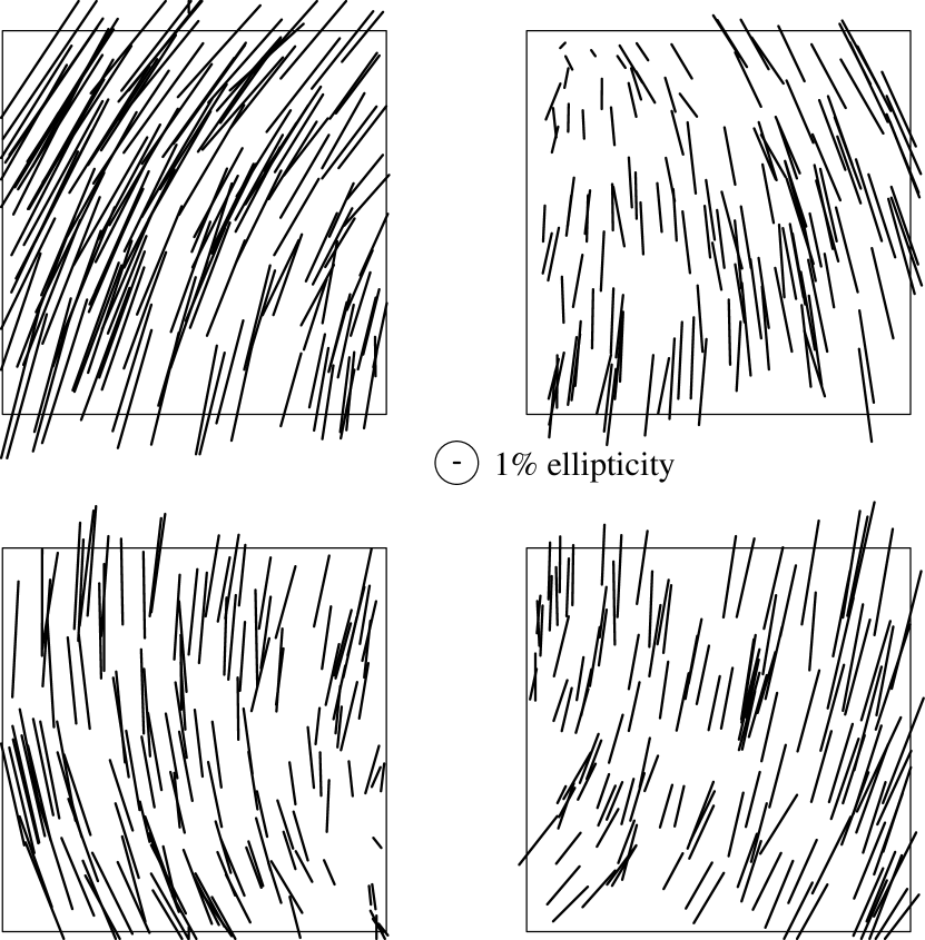
The most daunting problem in weak-lensing measurements is not the volume of the data, but rather the elimination of spurious shape correlations caused by instrumental effects, particularly asymmetric PSFs. Our decision to make a shallow survey is beneficial in that the galaxies have known $N(z)$ and larger angular sizes than faint galaxies, but a shallow survey has a smaller lensing signal and hence is more susceptible to systematic errors. Our requirements for rejection of systematic signals are very stringent: as noted below, the lensing distortion signal at our largest scales is $\approx 0.3\%$ RMS, while a large fraction of our images contain stellar images with ellipticities of 10% or higher. This is particularly a problem for the BTC images, because significant astigmatism in the telescope combines with warped CCDs to produce larger PSF ellipticities than is typical. Galaxies measured in image regions with stellar ellipticities $>0.25$ are discarded from the catalogs.

There are a number of checks one can make to look for systematic errors in the galaxy shapes. In particular, since the convolution should make the stars round, we check that the stars in the final image actually are round. Also, it is expected that most systematic effects will correlate with the position on the chips and/or the size and shape of the PSF. We describe here some of the tests we have done to quantify systematic errors which might remain after the processing steps described in §2.2.

2.3.1 Final Star Shapes

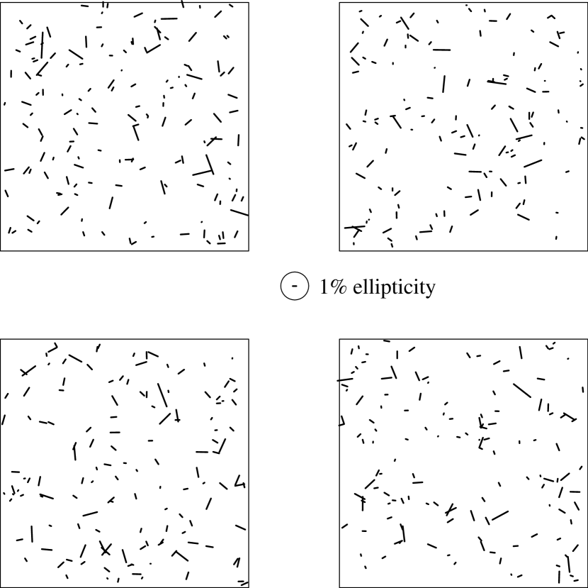
We make a “whisker plot” of the stars in every image to look for images where the processing may have gone wrong. For example, missed stars near the corners of the chip, a bad fit to the kernel, etc. A representative example of one of these plots along with the corresponding plot before the convolution is given in Figure 1. For reference, the horizontal whisker in the center of each corresponds to 1% ellipticity.

Clearly, the convolution does not make each star exactly round. Each whisker on the plot still has about 1-3% ellipticity. The important thing to check is that the convolution has removed any coherence in the whisker orientations. Measurement error on the stars’ ellipticities will leave uncorrelated random whiskers as residuals. The longer whiskers tend to correspond to fainter, noiser stars.

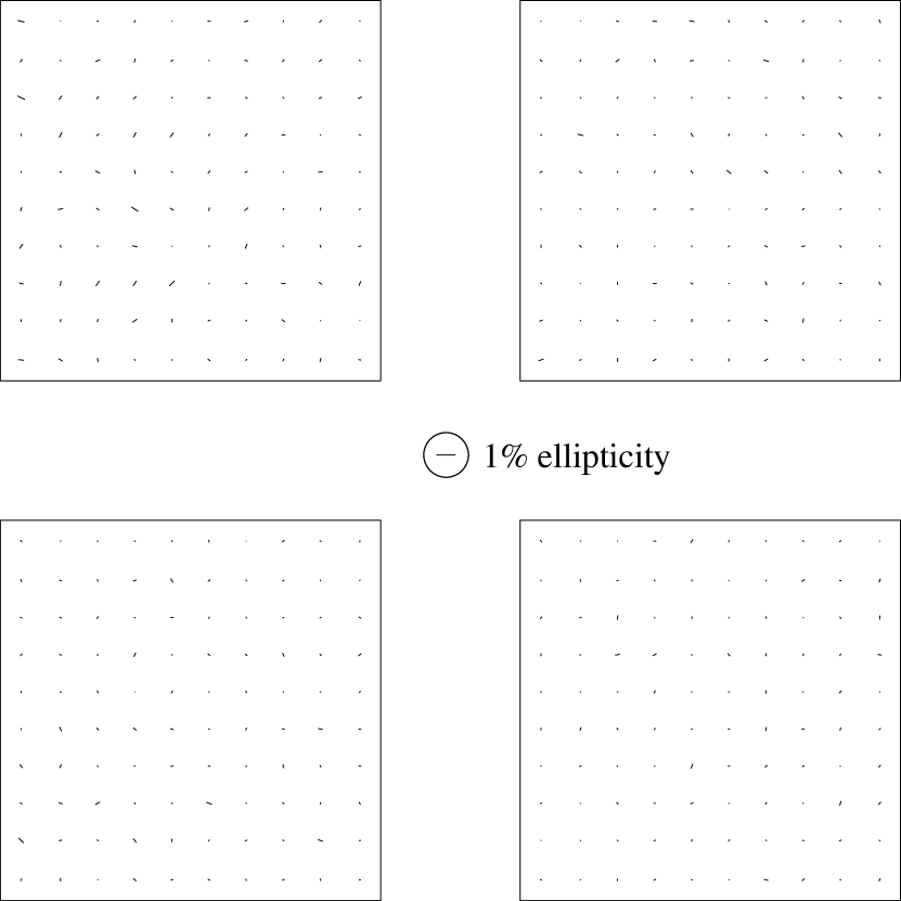
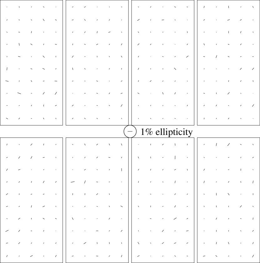
To search for residuals which may be coherent functions of pixel coordinates, we average the shapes of the stars from many images as a function of position on the CCD array. The whisker plots resulting from this procedure for both the BTC and Mosaic chips are shown in Figure 2.

All of the whiskers are smaller than the 1% whisker, with most of the whiskers barely visible ($<0.1\%$). The only whiskers which approach 1% in size are in the corners of the chips. This is mostly due to the fact that stars near the corners are more likely to be rejected from the kernel fits (in step 7 of §2.2). Therefore, fewer stars are being averaged, and the statistical errors tend to increase the resultant whisker size. This is not a problem for the galaxies, because galaxies in regions with no stars are also rejected.

Figure 2: Post-processing star shapes binned according to chip position for each of the BTC (left) and Mosaic (right) chips. The whiskers indicate the magnitude and orientation of this average shape. The central whisker in each plot corresponds to 1% ellipticity. The slight residuals which remain are well below the 1% level.

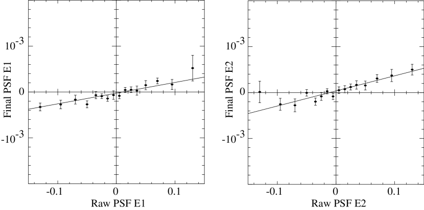
Another way to see how well we are making the stars round is to plot the final shape of the stars against the initial shape. This plot is shown in Figure 3. There is a noticeably positive slope for both $e_{+}$ and $e_{\times}$, but the slope is of order 1/300. This means that the shape of the PSF is reduced by a factor of 300 by the convolution. The mean final ellipticity for the worst initial ellipticities is less than 0.1%, which is well below the level of our lensing signal. Moreover, the rms deviation from zero is only 0.03%.

Figure 3: Final post-processing shapes of the stars binned according to their initial observed shape for each of the two components of the ellipticity. The fitted slope is of order 1/300, leaving an rms residual effect of 0.03% and a maximum effect of less than 0.1%, which is well below the strength of the lensing signal.

2.3.2 Galaxy Shape vs. Chip Position

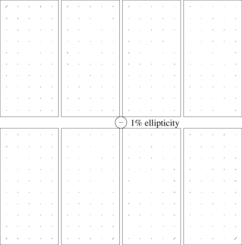
We can make whisker plots for the galaxies as well as the stars. The galaxies, however, are not each expected to be round after convolving. Even when the PSF is round, the galaxies each have a real shape variance of order 30%. To see if the convolution has affected the galaxies correctly as well as the stars, we reduce the shape noise by averaging the shapes of many galaxies. We first bin the galaxies by array position to search for systematic errors that depend upon pixel coordinates. Figure 4 shows the (null) results of this test. For neither hardware configuration do we detect any residual pattern in the galaxy shapes.

Figure 4: Post-processing galaxy shapes binned according to chip position for the BTC (left) and Mosaic (right) chips. For each shape observation, we subtract off the mean shape for that object as calculated from several observations from widely separated chip positions before binning. This removes the effect of shape noise. The central whisker in each plot corresponds to 1% ellipticity.

2.3.3 Galaxy Shape vs. PSF Shape

The biggest systematic effect to eliminate is the effect of the PSF. While there are other effects which vary across the chip, such as charge transfer inefficiencies, telescope distortion, and the flat field pattern, clearly the main concern is the PSF.

The most obvious test then is to bin the allegedly-corrected galaxy shapes by the “raw” PSF shape, as was done for the convolved stars. Again, each individual galaxy is not expected to be round, but the average shape of many galaxies should be independent of the PSF shapes for the galaxies if the survey is large enough to decouple the PSF variations from the true lensing signal. Figure 5 shows the results of this test.

Figure 5: Final post-processing galaxy shapes binned according to the PSF where they were observed. Clearly, there is still some bias relative to the PSF with a slope of order 0.015, which corresponds to a maximum bias of 0.4% for our worst PSFs, and a 0.2% rms effect. Note the greatly expanded vertical scale.

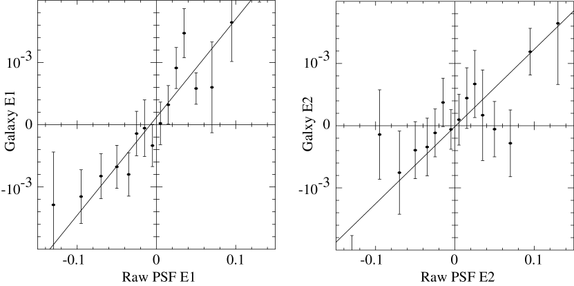
Apparently, there is still a bias of the galaxy shapes with respect to the initial PSF shape. The plot shows a slope of approximately 0.015, which corresponds to a 0.4% effect for our worst PSFs, and a 0.2% rms effect. This is somewhat below (but of the same order as) the level of our lensing signal.

We believe the observed residual galaxy dependence upon PSF shape is primarily due to higher-order asymmetries in the PSF which have not been removed by the $7\times 7$ convolution filters. We plan to implement the full higher-order analytical PSF corrections of BJ02 §6.3.5 and expect this to have smaller residuals than the kernel-convolution method used here.

Until then, we empirically fit for the slope of this bias and subtract the bias from the galaxy shape measurements. However, it is likely that simply subtracting the bias from the galaxy shapes is not the correct thing to do. In particular the bias seems to be stronger for faint galaxies and for large galaxies (which may be due to slightly non-linear CCD response or charge transfer efficiency). We currently use different bias slopes for $m>22$ and $m<22$, but it is possible that we have not correctly identified the exact population of galaxies which are giving us most of the bias. Therefore, we suspect that this residual is likely the main source of the B-mode power described in §3.4.

3 Analysis

3.1 Determining Shear from Shape Averages

Once we have a catalog of galaxy shapes, we want to be able to convert these shapes into various statistics of the lensing distortion field. These statistics require finding either the average of many ellipticities (e.g. the overall shear in each field, §3.2) or the average product of pairs of ellipticities (e.g. the shear correlation functions, §3.3).

The optimal weight for averaging ellipticities to obtain the lensing distortion [BJ02 Equation (5-28)] requires knowledge of the intrinsic distribution $P(e)$ of galaxy shapes. The distribution for the brighter, well-measured galaxies in this survey is shown in BJ02 Figure 4. BJ02 Equation (5-36) gives a simple weight which gives nearly optimal results:

$$w=[e^{2}+2.25\sigma_{\eta}^{2}]^{-1/2},$$ (2)

where $\sigma_{\eta}$ is the measurement uncertainty in each component of the shape, as measured in the sheared coordinate system where the shape is circular. BJ02 Figure 5 demonstrates that this weight recovers very close to the optimal signal to noise for the estimate of the distortion.

Thus, our estimate for a distortion from a set of shapes is (from BJ02 Equations 5-23, 5-33, and 5-35)

$$\hat{\mbox{\boldmath$\delta$}} =\frac{1}{\cal R}\frac{\sum w\,\mbox{\bf e}}{\sum w}$$ (3)

$${\rm Var}(\hat{\delta}_{i}) =\frac{1}{{\cal R}^{2}}\frac{\sum w^{2}e_{i}^{2}}{\sum w^{2}}\qquad(i\in\{+,\times\})$$ (4)

$${\cal R} =\frac{\sum\left[w\left(1-k_{0}-\frac{k_{1}e^{2}}{2}\right)+\frac{e}{2}\frac{dw}{de}\left(1-k_{0}-k_{1}e^{2}\right)\right]}{\sum w}$$ (5)

$$k_{0} =(1-f)\sigma^{2}_{\rm SN}$$ (6)

$$k_{1} =f^{2}$$ (7)

$$f =\frac{\sigma^{2}_{\rm SN}}{\sigma^{2}_{\rm SN}+\sigma^{2}_{\eta}}$$ (8)

The responsivity, ${\cal R}$, is similar to the shear polarizability of the KSB method and describes how our weighted mean ellipticity responds to an applied shear. In the simple case of an unweighted ellipticity average with unweighted shape measurements, ${\cal R}=1-\langle e^{2}\rangle=1-2\sigma^{2}_{\rm SN}$. The shape noise, $\sigma^{2}_{\rm SN}$, is the variance in the intrinsic $e_{+}$ of the galaxies. For our brighter galaxies, we measure $\sigma_{SN}=0.31$.

Figure 5 of BJ02 also demonstrates that the approximations made in the derivation of the above responsivity lead to $<1\%$ error in the resultant distortion calibration, for the shapes and noise levels of galaxies found in this survey. Smith et al. (2001) perform a complete numerical simulation of the distortion measurement process, concluding that the overall calibration is accurate to $\lesssim 5\%$. The BJ02 formulae improve upon those of Smith et al. (2001) so we believe the responsivity calibration is now accurate to $\approx 2\%$ or better.

3.2 Overall Shear in Each Field

The simplest statistic to calculate is the average distortion in each of our 12 fields. These results are listed in Table 2. The uncertainty on each of these measurements is typically $\pm 1\times 10^{-3}$. The $S/N$ for detection of each distortion component in each field is $\approx 2.5$. Collectively, they give a strong detection of the rms fluctuation in the shear field averaged on a scale of $2\fdg 5$. At the $z\approx 0.25$ redshift at which our sensitivity to lensing matter peaks (cf. §4.1), this corresponds to a comoving smoothing scale of $\approx 25h^{-1}$ Mpc, the largest scale to date on which gravitational lensing effects have been detected.

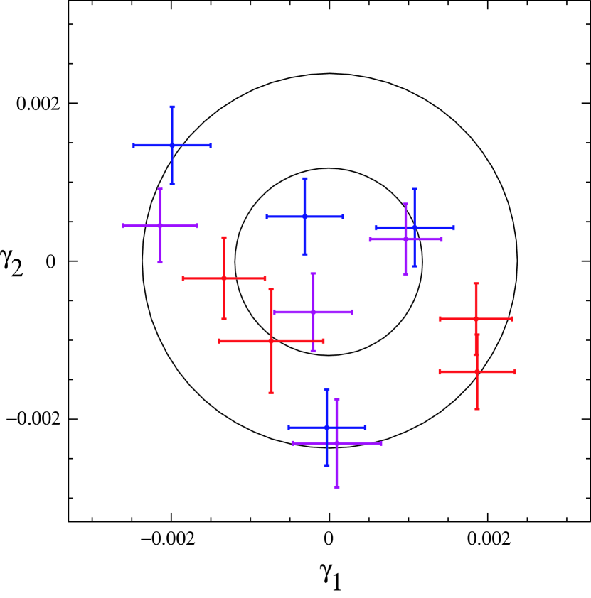
Figure 6 shows a scatter plot of the 12 distortion values, along with their error bars for each component. The mean distortions appear randomly distributed as expected for a real signal. A tendency to align on the $\delta_{+}$ axis would indicate a systematic error aligned with the CCD axes, such as charge transfer nonlinearities—no such effect is seen.

We assume that the average of each distortion component $\delta_{+}$ or $\delta_{\times}$ in a 2$\fdg$5 square box has a Gaussian probability distribution with width $\sigma$. The expected distribution is then broadened by the measurement error in each field (Equation (4)). A maximum likelihood analysis of the 24 values then yields $\sigma=0.0024\pm 0.0006$. Circles at 1$\sigma$ and 2$\sigma$ are also drawn on Figure 6 for reference. For comparison to other results which use the shear, $\gamma$, rather than the distortion, $\langle\gamma^{2}\rangle^{1/2}=\sigma/2=0.0012\pm 0.003$.

Figure 6: Scatter plot of the mean shear in each of the 12 fields. The distribution is found to be consistent with a Gaussian with $\sigma=0.0024\pm 0.0006$. This is in addition to the (assumed Gaussian) measurement errors. The red crosses are the Mosaic fields, blue are BTC, and purple are mixed.

3.3 Shear Correlation Functions

Miralda-Escudé (1991) introduced the shear correlation functions of the ellipticities of pairs of galaxies measured with respect to the line separating them. We will not make direct use of the correlation functions to constrain cosmology, but rather follow the prescriptions of Crittenden et al. (2002) (as clarified in Pen et al. (2002) and Schneider, van Waerbeke, & Mellier (2002a)) for constructing the $\langle M_{\rm ap}^{2}\rangle$ and $\langle\gamma^{2}\rangle$ statistics (described below) from the correlation function data.

The simplest way to calculate these functions is to treat the lens distortion as a complex number, $\delta=\delta_{+}+i\delta_{\times}$. To conform with other authors, we express the correlations in terms of the shear $\gamma$, related in the weak limit to the distortion by $\gamma=\delta/2$. Three correlation function are defined by:

$$\xi_{+}(\theta) =\langle\gamma({\bf r})\gamma^{*}({\bf r+\mbox{\boldmath$\theta$}})\rangle$$ (9)

$$\xi_{-}(\theta)+i\xi_{\times}(\theta) =\langle\gamma({\bf r})\gamma({\bf r+\mbox{\boldmath$\theta$}})e^{-4i\arg\theta}\rangle$$ (10)

Note that if the galaxies in a pair are swapped, the first equation turns into its conjugate. Thus, this quantity can be made manifestly real by double counting every pair of galaxies. With only single counting, the imaginary term gives an estimate of the statistical error of the other three quantities. Further, taking a mirror image of the entire field will turn the second equation into its conjugate. Thus, the imaginary part of this quantity is also expected to go to zero in the absence of systematic effects.

Near-optimal estimators for these two-point functions are constructed using the weight function and responsivity defined in Equations (2–8):

$$\hat{\xi}_{+}(\theta) =\frac{1}{4{\cal R}^{2}}\frac{\sum_{i,j}w_{i}w_{j}\delta_{i}\delta^{\ast}_{j}}{\sum_{i,j}w_{i}w_{j}}$$ (11)

$$\hat{\xi}_{-}(\theta)+i\hat{\xi}_{\times}(\theta) =\frac{1}{4{\cal R}^{2}}\frac{\sum_{i,j}w_{i}w_{j}\delta_{i}\delta_{j}e^{-4i\arg({\bf r}_{i}-{\bf r}_{j})}}{\sum_{i,j}w_{i}w_{j}}$$ (12)

where the sum is taken over all pairs of galaxies $i$ and $j$ with separation $\theta=|{\bf r}_{i}-{\bf r}_{j}|$ within some bin. The variance of $\hat{\xi}_{i}$ due to shape noise and shot noise is also simply estimated, but cosmic variance and bin covariances are more difficult to estimate. We bypass these complications by constructing field-to-field covariance matrices, as described below.

As our primary use of the correlation functions will be to calculate other quantities by integrating over a range of $\theta$, we calculate the correlation functions in fairly small bins with $\delta(\ln\theta)=0.05$.

3.4 Aperture Mass Statistic

The aperture mass statistic ($M_{\rm ap}$) is useful for estimating cosmological parameters. The idea is fairly straightforward: a mass concentration at the center of a given aperture will tend to produce a tangential pattern to the galaxy ellipticities around the center of the aperture. For cosmic shear measurements, we do not detect the mass concentrations individually [see Wittman et al. (2001) for a rare (so far) example], but rather the magnitude of the mass fluctuations, so we really want the rms variation of the $M_{\rm ap}$ value as the aperture is swept across the sky.

The $M_{\rm ap}$ statistic for a single aperture of radius $\theta$ is (Schneider et al., 1998)

$$M_{ap}(\theta) =\int_{0}^{\theta}d^{2}{\bf\phi}\,Q(\phi)\,\gamma_{t}({\bf\phi})$$ (13)

$$Q(\phi) =\frac{6}{\pi\theta^{2}}\frac{\phi^{2}}{\theta^{2}}\left(1-\frac{\phi^{2}}{\theta^{2}}\right)$$ (14)

where $\gamma_{t}$ is the tangential component of the shear (as estimated from the galaxy ellipticities). For many independent apertures, $\langle\mbox{$M_{\rm ap}$}\rangle=0$ and the variance, $\langle M_{\rm ap}^{2}\rangle$, probes the power spectrum of the effective convergence. The window function for this statistic is narrow in $k$-space and centered at $k\approx 4.1/\theta$ (Schneider et al., 1998).

One advantage of the $M_{\rm ap}$ statistic is that there is a natural test for systematics. If each galaxy is rotated in place by 45 degrees, the $M_{\rm ap}$ integral should vanish if due purely to lensing. This test is essentially measuring the curl of the shear field, and is therefore often called the “B mode,” while $M_{\rm ap}$ measures “E-mode” power. We designate this B-mode version of the $M_{\rm ap}$ statistic as $M_{\times}$. Most systematics are expected to add equal power to the E and B modes, hence the $M_{\times}$ data are a sensitive test for contaminating systematics.

Another advantage to using the $M_{\rm ap}$ statistic is that $M_{\rm ap}(\theta_{1})$ is very weakly correlated with $M_{\rm ap}(\theta_{2})$ when $\theta_{1}$ differs from $\theta_{2}$ by a factor of $\approx 2$ (Schneider et al., 2002). Thus, for our range of $1\arcmin<\theta<100\arcmin$, we have essentially 7 independent points with which to constrain cosmology.

The problem with calculating $\langle M_{\rm ap}^{2}\rangle$ in the obvious way (scanning the aperture across the images and calculating variance) is that each aperture is not uniformly filled with galaxies. There are holes due to foreground bright stars, edge effects, bad columns, etc. These holes can then bias the resulting $\langle M_{\rm ap}^{2}\rangle$ estimates and produce spurious $\langle M_{\times}^{2}\rangle$ power. Specifying a mask for our entire survey would require a painfully long time, as would the development of software to automate the task. Fortunately, Crittenden et al. (2002) (detailed also in Pen et al., 2002; Schneider, van Waerbeke, & Mellier, 2002a) express $\langle M_{\rm ap}^{2}\rangle$ and $\langle M_{\times}^{2}\rangle$ as integrals over the shear correlation functions, which do not require knowledge of the survey geometry. The relevant formulae are:

$$\langle M_{\rm ap}^{2}(\theta)\rangle =\frac{1}{2}\int_{0}^{2\theta}\frac{\phi\,d\phi}{\theta^{2}}\left[\xi_{+}(\phi)T_{+}\left(\frac{\phi}{\theta}\right)+\xi_{-}(\phi)T_{-}\left(\frac{\phi}{\theta}\right)\right]$$ (15)

$$\langle M_{\times}^{2}(\theta)\rangle =\frac{1}{2}\int_{0}^{2\theta}\frac{\phi\,d\phi}{\theta^{2}}\left[\xi_{+}(\phi)T_{+}\left(\frac{\phi}{\theta}\right)-\xi_{-}(\phi)T_{-}\left(\frac{\phi}{\theta}\right)\right]$$ (16)

where equations for $T_{+}$ and $T_{-}$ are given in Schneider, van Waerbeke, & Mellier (2002a). The result of this calculation for our data are shown in Figure 7 and discussed in the following sections.

Figure 7: Aperture mass and shear variance statistics measured on angular scales from 1 to 100 arcminutes. For the aperture mass statistic, the upper green line is the E-mode (lensing) signal, and the lower red line is the B-mode (non-lensing) signal. The light shaded region is bounded by E+B and E-B curves, representing the range of systematic uncertainty. Also plotted are the theory curves for our best fit model (dotted, dark blue), and for models at the high and low extremes of our 95% confidence limits quoted in Equation (32) (dotted, light blue). Points with error bars are given every factor of 2 in radius. For the $\langle M_{\rm ap}^{2}\rangle$ statistic, this is approximately the separation at which the data points are independent of each other.

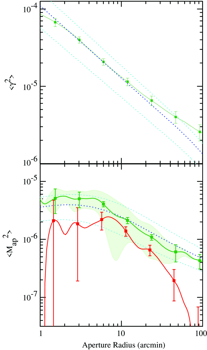
Another common statistic of the shear field is the windowed variance, $\langle\gamma^{2}(\theta)\rangle$, which is the variance of the shear when smoothed with a circular window of radius $\theta$. We have presented in §3.2 the results for the windowed shear in 2$\fdg$5 squares. For quantitative comparison to cosmological models, the naive $\langle\gamma^{2}(\theta)\rangle$ summation would require knowledge of the survey mask geometry. Again the above references show how to express $\langle\gamma^{2}(\theta)\rangle$ as an integral over $\hat{\xi}_{+}(\theta)$ and $\hat{\xi}_{-}(\theta)$, thereby removing the need to know the mask. If correlation function data are available out to separation $\theta_{\rm max}$, then all of $\langle M_{\rm ap}^{2}\rangle$, $\langle M_{\times}^{2}\rangle$ and $\langle\gamma^{2}\rangle$ are unambiguously determined for $\theta\leq\theta_{\rm max}/2$.

The $\langle\gamma^{2}\rangle$ statistic is inferior to $\langle M_{\rm ap}^{2}\rangle$ in several respects: its window function in $k$-space is much broader, and hence measurements at different $\theta$ are more highly correlated. Also $\langle\gamma^{2}\rangle$ does not separate E-mode from B-mode power, so the noise is $\sqrt{2}$ higher and there is no systematic-power null test. The information in this statistic is mostly degenerate with the $\langle M_{\rm ap}^{2}\rangle$ statistic, with the important exception that the variance probes the power spectrum for $k\lesssim 2/\theta$, whereas $\langle M_{\rm ap}^{2}\rangle$ probes $k\approx 4/\theta$. Therefore $\langle\gamma^{2}\rangle$ for $\theta$ near half our 2$\fdg$5 field size probes a portion of the power spectrum at larger physical scales than is accessible to $\langle M_{\rm ap}^{2}\rangle$. We will therefore make use of $\langle\gamma^{2}\rangle$ for $\theta>50\arcmin$. The $\langle\gamma^{2}\rangle$ statistic is plotted above the $\langle M_{\rm ap}^{2}\rangle$ statistic in Figure 7.

Pen et al. (2002) and Schneider, van Waerbeke, & Mellier (2002a) do give prescriptions for producing versions of the $\xi$ and $\langle\gamma^{2}\rangle$ statistics which separate the E and B contributions. However, these expressions have indeterminate constants of integrations which render the E and B modes degenerate on the scale of the field of view. Shear that is nearly constant over the field obviously cannot be classified as having either E or B properties. Since we only use $\langle\gamma^{2}\rangle$ for values of $\theta$ near the field size, we will not use this decomposition.

3.5 Covariance Matrix

For each of our twelve fields, we have a vector of observations, ${\bf x}_{n}\ (n=1,\ldots,12)$, including the $\langle M_{\rm ap}^{2}\rangle$ values from 1′ to 100′, and the $\langle\gamma^{2}\rangle$ values from 50′ to 100′. Each of these vectors has many data points, since we calculate each statistic at rather small intervals in aperture radius $\theta$. However, these data are highly degenerate in their information content. $\langle M_{\rm ap}^{2}\rangle$ values become essentially independent at a factor of 2 in $\theta$, giving only about 7 independent data points. And $\langle\gamma^{2}\rangle$ values are highly correlated with each other, with the effect that these values only add one more independent data point. So the mean of the twelve vectors, ${\bf x}=\langle{\bf x}_{n}\rangle$, gives us essentially 8 independent points with which to constrain cosmology.

To quantify this degeneracy more exactly, we construct the full covariance matrix, $\Sigma$, for the $N=12$ vectors by equally weighting each of the twelve fields:

$$\Sigma_{ij}=\frac{\sum_{n}[({\bf x}_{n})_{i}-\langle x_{i}\rangle][({\bf x}_{n})_{j}-\langle x_{j}\rangle]}{N(N-1)}$$ (18)

where $n$ ranges over the $N=12$ fields, and $i,j$ are the indices of the data values.

This construction of the covariance matrix means that we ignore the (approximately identical) nominal error bars for each point, using the actual field-to-field variation as our estimate of the error. This has the advantage that it automatically includes cosmic variance in the uncertainty as well as measurement noise both on and off the diagonal. The disadvantage is that the half-size fields, which have slightly larger statistical error bars, are given equal weight to the full-size fields.

3.6 B-mode Power

It is evident in Figure 7 that there is significant power in the $\langle M_{\times}^{2}\rangle$ statistic, indicating that we do have some B-mode power, and hence some systematic contamination in our data. The effect becomes much weaker at scales $\theta>30\arcmin$, suggesting that the large scale data are probably free of this contamination. Since the B-mode drops to essentially zero at the largest scales of $M_{\rm ap}$, we also expect that the $\langle\gamma^{2}\rangle$ statistic will be free of the contamination for $\theta>50\arcmin$, since it probes power at even larger angular scales.

Note that the observed B-mode signals are much larger than those to be expected from intrinsic galaxy-shape correlations (Crittenden et al., 2002) or second-order gravitational lensing effects (Schneider, van Waerbeke, & Mellier, 2002a; Cooray, 2002). We believe that they are more likely due to uncorrected high-order PSF effects or inexact kernel fitting, both of which become more important at smaller scales.

Most systematics effects, including uncorrected PSF variation, can increase $\langle M_{\rm ap}^{2}\rangle$ and $\langle M_{\times}^{2}\rangle$ much more easily than decrease. However, one can also conceive of systematic effects which simply mix power from the E-mode into B-mode rather than add power to either one. For example, if each ellipticity vector’s orientation is rotated slightly but the magnitude is unchanged, then no power is added, but the power is mixed somewhat into the B-mode.

Therefore, a conservative estimate is that the $\langle M_{\rm ap}^{2}\rangle$ values can be in error in either direction by the amount of the $\langle M_{\times}^{2}\rangle$ values. Further, it is not sufficient to simply increase the error bars on individual data points by this amount, since the effect is presumably in the same direction at all (or many) values of $\theta$. Instead, one should consider the two cases of adding the B-mode to all points and of subtracting it from all points. The range of these two cases will then give an estimate of the full potential effect of the systematic error. If the spurious systematic signal has more E power than B power, we could still have overestimated the lensing E signal. Such behavior is expected only, however, for intrinsic correlations, which we believe to be a small constituent of our systematic contamination.

In any case, for the purpose of constraining cosmology, we want to limit our consideration to the range of $\theta$ that has the least amount of B-mode contamination. We will use the $\langle M_{\rm ap}^{2}\rangle$ values only for $30\arcmin<\theta<100\arcmin$, and still use $\langle\gamma^{2}\rangle$ from $50\arcmin<\theta<100\arcmin$. Thus, our data vectors ${\bf x}_{k}$ (cf. §3.5) now only have essentially 4 independent data points. The increase in the statistical error from this reduced $\theta$ range is however much more than compensated by the decrease in the systematic error from the B-mode; in this range the systematic error is smaller than the statistical error.

Table 3: Data Used for Cosmological Constraints

	E-Mode	$\sigma_{E}$	B-Mode	$\sigma_{B}$	Reduced Covariance Matrix
	$\times 10^{-7}$		$\times 10^{-7}$			($\Sigma_{ij}/\sigma_{i}\sigma_{j}$)
$\mbox{$\langle M_{\rm ap}^{2}\rangle$}(30\arcmin)$	9.52	1.38	3.44	1.25		1	0.80	0.20	-0.13
$\mbox{$\langle M_{\rm ap}^{2}\rangle$}(50\arcmin)$	7.24	2.00	1.23	1.19		0.80	1	0.14	0.02
$\mbox{$\langle M_{\rm ap}^{2}\rangle$}(100\arcmin)$	3.84	1.09	-0.21	1.00		0.20	0.14	1	-0.11
$\mbox{$\langle\gamma^{2}\rangle$}(100\arcmin)$	26.4	6.20	-	-		-0.13	0.02	-0.11	1

Figure 8: Window functions for each of the statistics listed in Table 3, as defined in Equation (19). From left to right, the curves are for $\mbox{$\langle\gamma^{2}\rangle$}(100\arcmin)$ (black), $\mbox{$\langle M_{\rm ap}^{2}\rangle$}(100\arcmin)$ (red), $\mbox{$\langle M_{\rm ap}^{2}\rangle$}(50\arcmin)$ (green), and $\mbox{$\langle M_{\rm ap}^{2}\rangle$}(30\arcmin)$ (blue).

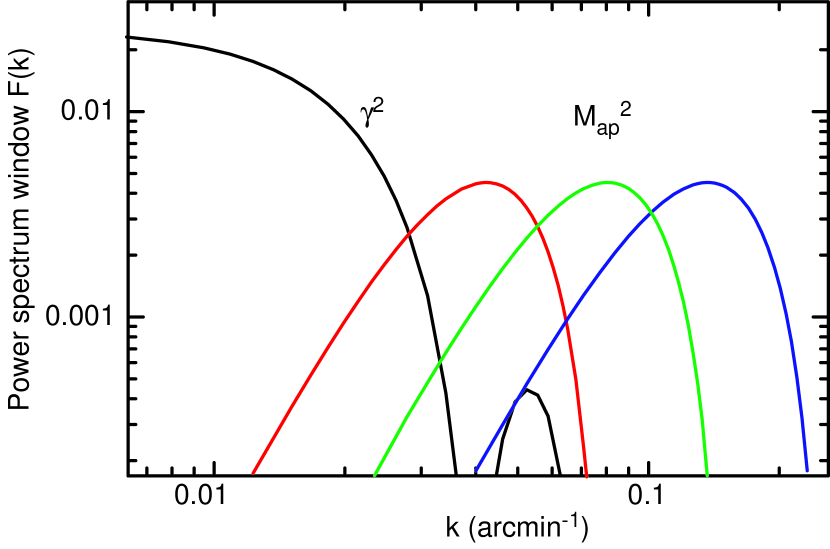
For reference, an abridged listing of the data and covariance matrix is given in Table 3. It includes both the shear variance and the aperture mass statistics (both E and B mode in the latter case) for selected values within this range. It also gives the reduced covariance matrix as described in §3.5 for these values. It is evident that the four statistics are relatively uncorrelated with only $\mbox{$\langle M_{\rm ap}^{2}\rangle$}(30\arcmin)$ and $\mbox{$\langle M_{\rm ap}^{2}\rangle$}(50\arcmin)$ being somewhat correlated. This is expected, since they sample the power spectrum at relatively disjoint ranges in frequency. Each statistic can be written:

$$y_{i}=\int kdkP_{\kappa}(k)F_{i}(k\theta)$$ (19)

and Figure 8 shows $F_{i}$ for each of these four statistics.

4 Cosmological Implications

4.1 Redshift Distribution

In BJ02 it is shown that the distortion estimators in §3.1 will converge to the lensing distortion. In reality the expected distortion $\delta(z)$ is a function of the source redshift $z$, and we determine some mean distortion $\bar{\delta}$. We do not know the redshift $z_{i}$ of every source galaxy, but we can have some knowledge of its distribution vs. magnitude $P(z|m)$ from spectroscopic redshift surveys. If we divide our source galaxies into redshift bins $Z_{j}$ then the measured signal should converge to

$$\bar{\delta}=\langle\hat{\delta}\rangle =\frac{\sum_{i}w_{i}e_{i}}{\sum_{i}w_{i}{\cal R}_{i}}$$ (20)

$$=\frac{\sum_{j}\left[\left(\sum_{z_{i}\in Z_{j}}w_{i}\right)\frac{\sum_{z_{i}\in Z_{j}}w_{i}{\cal R}_{i}}{\sum_{z_{i}\in Z_{j}}w_{i}}\frac{\sum_{z_{i}\in Z_{j}}w_{i}e_{i}}{\sum_{z_{i}\in Z_{j}}w_{i}{\cal R}_{i}}\right]}{\left(\sum_{i}w_{i}\right)\frac{\sum_{i}w_{i}{\cal R}_{i}}{\sum_{i}w_{i}}}$$ (21)

$$=\frac{\sum_{j}w(Z_{j}){\cal R}(Z_{j})\delta(Z_{j})}{\sum_{j}w(Z_{j}){\cal R}(Z_{j})}.$$ (22)

Here we have defined $w(Z_{j})$ to be the total weight in the redshift bin, and ${\cal R}(Z_{j})$ is the mean responsivity, as per Equation (5), of the galaxies in the bin. We will make the assumption that ${\cal R}$ is independent of redshift. For galaxies with magnitude $R<21$, we do see a significant dependence of the effective ${\cal R}$ upon surface brightness, with $0.62>{\cal R}>0.75$ as we select subsets of extremely high or low surface brightness and high or low measurement noise. On the other hand, each redshift bin contains galaxies with a wide range of surface brightness and measurement noise, so the responsivity variation with $z$ should be much smaller than this extreme $\pm 10\%$ range.

With the ${\cal R}$ taken as constant, the measured distortion (22) becomes

$$\bar{\delta} =\frac{\sum_{i}w_{i}\delta(z_{i})}{\sum_{i}w_{i}}$$ (23)

$$=\frac{\int\!dz\int\!dw\int\!dm\,\delta(z)wP(z,w,m)}{\int\!dz\int\!dw\int\!dm\,wP(z,w,m)}$$ (24)

where $P(z,w,m)$ is the probability of a given galaxy having redshift $z$, weight $w$, and apparent magnitude $m$. Ideally we would determine the function $P$ by conducting a redshift survey over a statistically significant sample of galaxies with known $m$ and $w$ for our survey conditions. Existing surveys, however, can only give us the conditional distribution $P(z|m)$ of redshift for a given magnitude. We will therefore make the further assumption that, within a given magnitude bin, the redshift $z$ [or more precisely $\delta(z)$] is statistically independent of the weight $w$, so that $\langle\delta(z)wP(z,w|m)\rangle=\langle\delta(z)P(z|m)\rangle\langle wP(w|m)\rangle$, in which case

$$\bar{\delta}=\frac{\int\!dm\,P(m)\left[\int\!dz\,\delta(z)P(z|m)\right]\left[\int\!dw\,wP(w|m)\right]}{\int\!dm\,P(m)\int\!dw\,wP(w|m)}$$ (25)

Since the redshift data are sparse, the integrals are calculated in 0.5-magnitude bins. Let the lensing survey field contain a total weight $W(m)$ of galaxies in the magnitude bin, which we apportion among the $N(m)$ galaxies in the redshift survey that lie within this bin. If redshift-survey galaxy $i$ has redshift $z_{i}$ and lies in magnitude bin $m_{i}$, then the expected signal becomes

$$\bar{\delta} =\sum_{i}\delta(z_{i})W_{i}$$ (26)

$$W_{i} \equiv\frac{W(m_{i})/N(m_{i})}{\sum_{i}W(m_{i})/N(m_{i})}$$ (27)

Figure 9: The total relative weight of our galaxies for each of our 12 fields as a function of magnitude. The weight function is quite similar up to $m=22$, at which point they begin to diverge. We cut our catalogs at $m=23$ to minimize variations in depth from field to field.

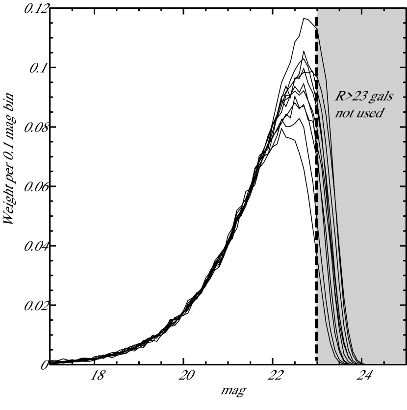
Figure 9 plots the distribution of weight vs. magnitude for galaxies which pass the selection criteria in step 10. Each of the 12 fields are plotted separately. We truncate the galaxy sample at $R<23$ to minimize field-to-field variations in effective depth, and to keep the galaxy sample to the magnitude range for which sizable redshift surveys are available. We also truncate at $R>19$, since bright galaxies are negligibly lensed.

The Caltech Redshift Survey (Cohen et al., 2000)[CRS] is almost complete for ${\cal R}=23.5$ for a 437 galaxy sample surrounding the Hubble Deep Field. The Steidel & Hamilton (1992) ${\cal R}$ photometric system (not to be confused with our symbol for responsivity) differs slightly in both zeropoint and bandpass from the $R$ system defined by Landolt (1992). Convolution of synthetic galaxy spectra at a variety of redshifts (R. Somerville, private communication) suggests that $\langle R-{\cal R}\rangle\approx 0.18$ mag for $z<0.3$ or $z>1$ galaxies, rising to $\langle R-{\cal R}\rangle\approx 0.37$ mag at $z\approx 0.7$ as the 400 nm break in galaxy spectra moves between the two filters. We apply this correction to the CRS ${\cal R}$ magnitudes to define an $R<23$ sample that is 97% complete. The CRS magnitudes are then corrected for Galactic extinction in the same way as our program fields.

We apply Equation (26) to this CRS sample, assuming that either (a) all the galaxies with unknown redshift are at $z=1$, or (b) galaxies with unknown redshift have the same $z$ distribution as other galaxies of similar magnitude. For the underlying weight distribution, we take that of the field of median depth, field T. We also examine the effect of taking the shallowest (A) and deepest (N) fields. Choosing case (a) or (b) for incompleteness, or fields T, A, or N, changes the expected $\langle M_{\rm ap}^{2}\rangle$ signal by at most 4% from the canonical case. The implied uncertainty in $\sigma_{8}$ is, at 2%, insignificant compared to the measurement errors.

A calibration of our signal can also be done using the Canada-France Redshift Survey (Lilly et al., 1995)[CFRS], which is complete to $I_{AB}<22.5$. While $R$-band magnitudes are not measured in the CFRS, Smith et al. (2001) collect $R$-band images in the CFRS fields so that a $R<23$ sample of 783 galaxies can be defined, after correcting for Galactic extinction in the CFRS fields. This $R<23$ subset of the CFRS sample is not quite representative of our source galaxies because the bluer galaxies at $R\approx 23$ do not make the $I_{AB}<22.5$ cut of the CFRS sample. The CFRS $R<23$ sample is also only 88% complete in redshift. The incompleteness in redshift and the depth/color mismatch make the CFRS data less reliable for our purposes than the CRS. Nonetheless, treating the incompleteness by method (a) above ($z=1$) gives a calibration within 5% of the nominal CRS case. Using method (b), however, gives an expected $\langle M_{\rm ap}^{2}\rangle$ signal that is 15% below that of the nominal CRS value. Given the known shortcomings of the CFRS sample, we will take this as a very conservative 95% CL bound on the possible error of the CRS depth calibration. Since $\mbox{$\langle M_{\rm ap}^{2}\rangle$}\propto\sigma_{8}^{2.2}$ at our larger scales, the 95% CL error on $\sigma_{8}$ is 7%, to be added in quadrature with the statistical errors and B-mode corrections.

Figure 10: Sensitivity of our survey to mass fluctuations, plotted as a function of the lens redshift. The underlying source distribution is inferred from the Caltech Redshift Survey (solid) or Canada-France Redshift Survey (dashed) as detailed in the text. Galaxies with unknown redshifts in these surveys are assumed to be either at $z=1$ (upper, black) or distributed as the other galaxies (lower, red). The differences between these curves correspond to a maximum of 7% uncertainty on the power spectrum normalization $\sigma_{8}$.

There is an additional uncertainty due to our assumptions that ${\cal R}$ and $P(w|m)$ are independent of redshift. Note that this assumption is implicit in all previous cosmic-shear measurements. A detailed test of this assumption requires larger redshift surveys, and we will for the time being ignore the effect as we believe it is weak.

4.2 Prediction of Signals

Using the notation of Schneider et al. (1998), and approximating the source distribution as a set of weighted delta functions at the observed redshift-survey $z$’s, the angular power spectrum of the lensing convergence is expected to be

$$P_{\kappa}(k)=\frac{9}{4}\Omega_{0}^{2}\int_{0}^{w_{H}}\frac{dw}{a^{2}(w)}P_{3D}\left(\frac{k}{f_{K}(w)};w\right)\left[\sum_{i}W_{i}\frac{f_{K}(w_{i}-w)}{f_{K}(w_{i})}\right]^{2}.$$ (28)

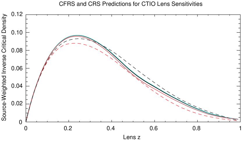
Here $w$ is the conformal distance from $z=0$, $w_{H}$ is the horizon, $w_{i}$ are the distances to the redshift-survey galaxies, $f_{K}$ is the comoving angular diameter distance, and $P_{3D}$ is the mass power spectrum at a given comoving scale and epoch. Figure 10 plots the bracketed quantity in Equation (28) [with an additional factor of $f_{K}(w)$] as a function of the lens redshift $z_{l}$, for several of the assumptions about source-galaxy redshift distributions detailed above—they are all seen to give very similar results. The sensitivity function has a broad peak at $z\approx 0.25$.

There are two important issues in making model predictions for the $\langle M_{\rm ap}^{2}\rangle$ and $\langle\gamma^{2}\rangle$ statistics. First, for the angular scales of interest, nonlinear clustering and its evolution must be taken into account. Jain & Seljak (1997) show that the effect of nonlinear enhancement exceeds a factor of 4 in the variance on arcminute scales, and is about 50% at 10′ (for $\sigma_{8}$ close to unity). Thus essentially all existing shear-correlation measurements in the literature probe the nonlinear regime. Since our survey measurements extend to beyond 1 degree (albeit at shallower depth), we span an interesting dynamic range that includes the nonlinear regime (below 5 arcminutes), the quasilinear (10-20 arcminutes) and the nearly linear regime on larger scales. In any case, to compare our full set of measurements to model predictions with some degree of accuracy requires that we use a well calibrated model for the nonlinear mass power spectrum. The fitting formulae developed by Hamilton et al. (1991); Peacock & Dodds (1994); Jain, Mo & White (1995); Peacock & Doods (1996) provide empirical but fairly accurate predictions for the nonlinear power spectrum. We will use the Peacock & Doods (1996) formulae to compute the shear variances for different models. Recently vW02 have discussed the accuracy achieved with these formulae and found that on arcminute scales there is some uncertainty in the theoretical predictions which precludes parameter estimation at much better than the 10% percent level. The large angular scale coverage of our measurements makes this uncertainty on small scales less of an issue.

The second issue in making model predictions is the choice of cosmological parameters to vary. One approach is to choose a physical model and vary parameters that have specific meaning within such a model. Our approach however will be closer to an empirical one in which we will choose the parameters that lensing is most sensitive to and take other parameters to be unknown or fixed. Based on earlier theoretical work (Kaiser, 1992; Bernardeau et al., 1997; Jain & Seljak, 1997), we choose the primary parameter space to be that of $\sigma_{8}$, such that the amplitude of the linear power spectrum is $\propto\sigma_{8}^{2}$, and $\Omega_{m}$, the present mean mass density parameter of the universe. We will parameterize the shape of the power spectrum by the standard $\Gamma$ parameter, which has a specific physical meaning for cold dark matter models. We will fix $\Gamma=0.21$ and the primordial spectral index $n=1$ in most of the analysis, but as discussed below, we will explore the sensitivity of our constraints to the value of $\Gamma$. We have above explored the sensitivity to the uncertainty in our redshift distribution. Our analysis is similar in spirit to that of vW02, but our choice of survey depth and angular scale makes the interpretation insensitive to unmeasured parameters of $N(z)$ and $\Gamma$, so marginalization over these quantities is not required.

The theoretical predictions for $\langle\gamma^{2}\rangle$ and $\langle M_{\rm ap}^{2}\rangle$ are given by the following equations:

$$\langle\gamma^{2}(\theta)\rangle =\frac{2}{\pi\theta^{2}}\int_{0}^{\infty}\frac{dk}{k}P_{\kappa}(k)J_{1}(k\theta)^{2},$$ (29)

$$\langle M_{\rm ap}^{2}(\theta)\rangle =\frac{288}{\pi\theta^{4}}\int_{0}^{\infty}\frac{dk}{k^{3}}P_{\kappa}(k)J_{4}(k\theta)^{2},$$ (30)

where $J_{1}$ and $J_{4}$ are the first and fourth-order Bessel functions, and $P_{\kappa}$ is given by Equation (28). In the linear regime, for an Einstein-de Sitter universe the 3-dimensional mass power spectrum grows in time as $a^{2}$, so the dependence on the redshift coordinate $w$ is contained in the term in square brackets in Equation (28). However for other cosmologies and in the nonlinear regime the growth rate is different, so the dependence on $w$ is more complicated and can be scale dependent. Thus the dependence on cosmological parameters enters in rather complicated ways through the distance factors as well as the power spectrum. For a reasonable class of models that are at all consistent with other cosmological probes, the dependence of the second moment of lensing statistics on the cosmological constant is weak. The main dependences then are on $\Omega_{m}$ and $\sigma_{8}$, and as shown in previous work, the combination that enters is close to the one in cluster abundances and is given roughly by $\langle\gamma^{2}\rangle\propto\sigma_{8}^{2}\Omega_{m}$. There are further dependences on the shape of the power spectrum and the redshift distribution which we will explore below.

4.3 Fit of Models to the Data

As described in §3.5 above, our data are essentially reduced to a mean vector, ${\bf x}$, of $\langle M_{\rm ap}^{2}\rangle$ and $\langle\gamma^{2}\rangle$ values, along with the covariance matrix of these values, $\Sigma$. We calculate the corresponding vector for each of our cosmological models and compute a $\chi^{2}$ value for each model:

$$\chi^{2}=\left({\bf x_{data}}-{\bf x_{model}}\right)\mbox{\boldmath$\Sigma$}^{-1}\left({\bf x_{data}}-{\bf x_{model}}\right)$$ (31)

One important consideration in the above calculation is that our covariance matrix is largely degenerate. Our vector has over 100 elements, since we calculate the statistics at fairly small separations in aperture radius. However, as discussed in §3.5 and §3.6, there are really only 3–4 independent data points among all of these. Rather than selecting 4 values of $\theta$ arbitrarily, we use a singular value decomposition to calculate $\mbox{\boldmath$\Sigma$}^{-1}$, and take only the largest 4 eigenvalues of the decomposition. This automatically uses only the non-degenerate components of the matrix, and in some sense finds the best combination of the data to use for our 4 values. The 4 values selected for Table 3 are therefore merely representative of the data used for the constraints.

Figure 11 shows a contour plot of $\chi^{2}$ as a function of $\Omega_{m}$ and $\sigma_{8}$. The nominal overall best fit is at $\sigma_{8}=0.37,\Omega_{m}=0.82$. However, there is clearly a strong degeneracy in this plot indicating that we really only constrain the combination $\sigma_{8}\Omega_{m}^{0.57}$, which is found to have a value of $0.334\pm 0.040$ (95% confidence interval).

Figure 11: Contour plots of $\chi^{2}$ of our data as a function of $\Omega_{m}$ and $\sigma_{8}$, assuming $\Lambda$CDM, $\Gamma=0.21$. The left plot uses the data as measured, taking only the E-mode signal for the $M_{\rm ap}$ statistic. For the middle plot, the B-mode signal has been added to the E-mode. And for the right plot, the B-mode signal has been subtracted from the E-mode. Contours in all cases are drawn at 1, 2, and 3 sigma, which correspond to $\Delta\chi^{2}$ = 2.30, 6.17, and 11.8 for two parameters. Marginalizing down to one parameter yields tighter 1-dimensional uncertainty intervals. We also include our final 95% confidence range for $\Omega_{m}=0.3$ (from Equation (32)) on each plot for reference.

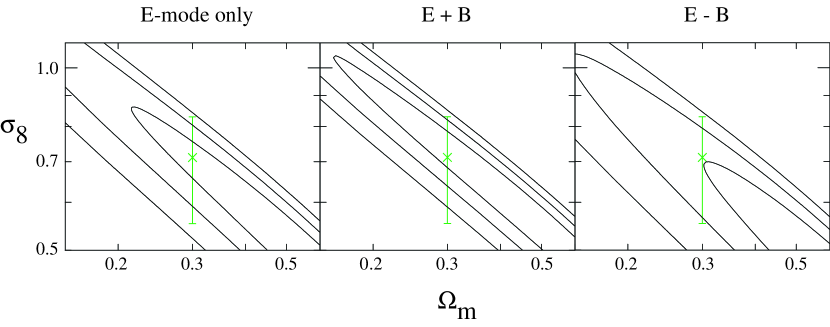
This error bar includes only the statistical and cosmological variations which went into the calculation of the covariance matrix. However, we need to account for the systematic uncertainty due to the B-mode power. As discussed above in §3.6, we allow for the two possibilities: that the E-mode should be either increased or decreased by the amount of the B-mode. For these two extremes (also plotted in Figure 11), we find that $\sigma_{8}\Omega_{m}^{0.57}$ ranges from 0.263 to 0.377 at the 95% confidence level. That is, these are the minimum and maximum values at 95% confidence for any of the three cases: E, E+B or E-B. These values then span the full range allowed by our data taking into account both the systematic and the statistical errors.

Our calibration and redshift uncertainties of  5% and  7% respectively are smaller than the above errors but need to be included. We also examined the dependence of our result on $\Gamma$, and found that for the range [0.15,0.50], our estimate of $\sigma_{8}$ varied as $\Gamma^{-0.02}$, which even for the extremes of this range is only a 2% result, and is therefore negligible compared to our other uncertainties.

We add all of these uncertainties in quadrature to get a final estimate of:

$$\sigma_{8}\left(\frac{\Omega_{m}}{0.3}\right)^{0.57}=0.71^{+0.12}_{-0.16}\quad\hbox{(95\% CL)}$$ (32)

which includes all systematic, statistical, and calibration uncertainties.

Models for the high and low extremes of this range along with the best fit model are the dotted curves plotted in Figure 7.

4.4 Potential Causes of the B-Mode

It is particularly unfortunate that we cannot use the data at $\theta<30\arcmin$, since one of the expected benefits from our survey was the large dynamic range over which we are able to measure shear. We make a significant lensing detection from $1\arcmin$ up to $\gtrsim 150\arcmin$, over 2 decades of power-spectrum range. In the absence of contaminating power, our uncertainty in $\sigma_{8}$ would be approximately half of our present error bar. The benefit of having a larger scale range is that it can break the degeneracy seen in Figure 11 between $\sigma_{8}$ and $\Omega_{m}$. Larger values of $\Omega_{m}$ tip the predicted curve up at small scales, whereas smaller values tip it down. So with the full range of data and no B-mode contamination, we would start to gain some constraint on $\Omega_{m}$.

If we repeat the above calculation using the entire range of 1′–100′ for the $\langle M_{\rm ap}^{2}\rangle$ statistic and the same 50′–100′ for the $\langle\gamma^{2}\rangle$ statistic, we find that the statistical error bars drop from about 17% to about 7%. However, the systematic errors dominate in this case, so that the final 95% CL estimate is $\sigma_{8}(\Omega_{m}/0.3)^{0.47}=0.75^{+0.23}_{-0.17}$. Thus, while the statistical precision is nominally improved, the B-mode degrades the expected accuracy, and therefore we believe the above estimate (Equation (32)) is more appropriate.

Given the obvious benefits to removing whatever is causing the B-mode contamination, we have spent considerable time trying to determine the cause and which steps have brought the B mode down to its current level. A detailed discussion is in Jarvis (2002), which we summarize here.

One step which we believe is a source of spurious power is the fit of the kernel across the image (§2.2, step 7). We found the B-mode to drop somewhat when we switched from a polynomial fit to a smoothing spline. There are unfortunately only $\approx 100$ stars per image, which means that even without noise, a fit can only probe variations on scales larger than $\approx 1/10$ of the chip size ($\approx 1.5\arcmin$). Smoothing the PSF fit to average measurement noise means that real variations in the PSF on scales of several arcminutes will be missed.

Another source of spurious power could be higher-order asymmetries left in the PSF after application of our circularization kernel. We currently use a $7\times 7$ kernel which removes the lowest 3 orders of the PSF bias. Stars in our fields do have significant power in higher orders. We tried to test this hypothesis by increasing our kernel size from $5\times 5$ to $7\times 7$ (which we still use here), but the B-mode did not change significantly.

Figure 12: E and B mode curves for the 4 fields which were taken with the BTC camera, the 4 taken with the Mosaic camera, and the 4 mixed fields. The three types of fields are seen to be generally consistent with each other, although there is some indication that the BTC fields may have slightly more power. It is also important to note that none of the three types of fields have significant B-mode power at $\theta>30\arcmin$.

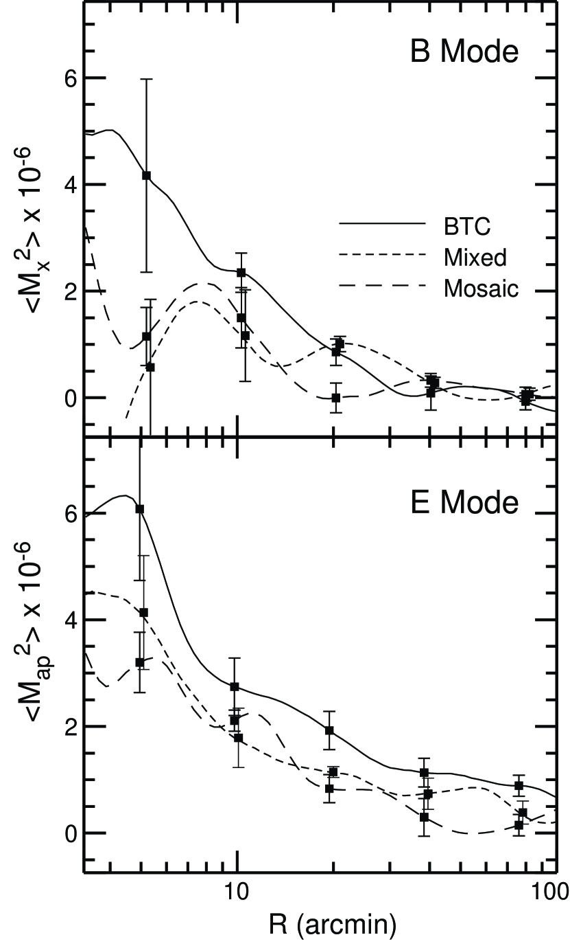
Non-linearities in the CCD response could produce spurious shear power, because we use relatively bright stars to measure the size and shape of the PSF. If this were the case, however, the effect would likely be very different for the two cameras used in our observations. The measured E and B powers for BTC, Mosaic, and mixed fields are all consistent with each other, as illustrated in Figure 12.

While we do not know which of the above effects is causing our B-mode, shortcomings in the PSF-circularization kernel seem the most likely cause. We may be able to do better by implementing the analytic deconvolution technique described in BJ02.

To be complete, there is another possible cause of the B-mode contamination—intrinsic correlations of the galaxy ellipticities. Crittenden et al. (2001) calculate the correlation function that may exist due to spin correlations between galaxies. The predicted power, scaled to our median redshift of 0.5, is not much lower than the B-mode power seen in our data. They indicate in their conclusions that there are a number of reasons to suspect that the predictions are an overestimate of the true power from intrinsic correlations; however, it is possible that a large portion of our B-mode power is due to this effect. Note that if this is the case, then Crittenden et al. (2002) calculate that the power should be approximately evenly split between the E-mode and B-mode, in which case, the E-B fit above is the appropriate one for weak lensing constraints.

4.5 Consumer’s Guide to Current Weak Lensing Results

Table 4 lists some of the most recent weak-lensing results, quoting the value of $\sigma_{8}$ at $\Omega_{m}=0.3$ and $\Gamma=0.21$ in order to make the comparisons more obvious. Note, however, that all authors actually constrain a parameter $\sigma_{8}\Omega_{m}^{\alpha}\Gamma^{\beta}$, where $\alpha$ is usually $\approx$ 0.4–0.6, and $\beta$ ranges from -0.02 for our survey (cf. §4.3) to 0.15 for Refregier et al. (2002). Our result is clearly somewhat lower than the other recent $\sigma_{8}$ values, but the relatively large error bars for most of these are such that we are nominally consistent with all of them (although we are only barely consistent with vW02 at 95% confidence).

Table 4: Recent Weak Lensing Measurements of $\sigma_{8}$

	$\sigma_{8}$	Mag Limit	${\bar{z}}$	Max scale	Survey Area	B Mode?	$N(z)$	$\Gamma$
	(95% CL)		(source)	(arcmin)	(sq. deg.)
This Work	$\mbox{0.71}^{+\mbox{\scriptsize 0.12}}_{-\mbox{\scriptsize 0.16}}$	$R<23$	0.66	100	75	yes	spectroscopic	irrelevant
Hamana et al. (2002)	$\mbox{0.69}^{+\mbox{\scriptsize 0.41}}_{-\mbox{\scriptsize 0.22}}$	$I<24.5$	$\sim 1$	40	2.1	yes	marginalized	marginalized
Brown et al. (2002)	0.74$\pm$0.18	$R<24$	0.85	15	1.25	yes	photometric	$\Gamma=0.72\Omega_{m}$
Hoekstra et al. (2002)	$\mbox{0.86}^{+\mbox{\scriptsize 0.08}}_{-\mbox{\scriptsize 0.10}}$	$R<24$	0.58	50	53	yes	marginalized	marginalized
Van Waerbeke et al. (2002)	0.96$\pm$0.23	$I<24.5$	0.84	30	8.5	yes	marginalized	marginalized
Bacon et al. (2002)	0.97$\pm$0.26	$R<25.8$	0.9	12	1.6	unknown	photometric	$\Gamma=0.21$
Refregier et al. (2002)	0.94$\pm$0.28	$I<24.5$	0.95	1.4	0.04	unknown	photometric	$\Gamma=0.21$

Direct comparison of various results is complicated, however, because the uncertainties included in the error bar vary, even though all the error bars are 95% confidence. We note here some of the important distinctions between current results which must be considered when making detailed comparisons. Table 4 serves as a “scorecard” for recent cosmic-shear results.

• Statistical and Cosmic Variance: Uncertainties in shear power estimates of all the papers in Table 4 include the contributions of random (shape) noise and cosmic variance. For vW02 and RRG02 these are estimated analytically. The other authors use measured field-to-field covariance matrices, which will automatically include shape noise and cosmic variance.

  

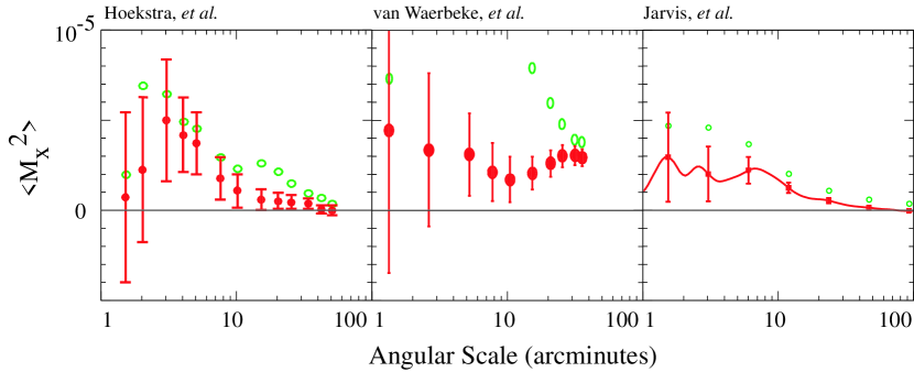
  Figure 13: Measurements of the B-mode contamination from each of the three surveys which have tested for it so far. The left panel is taken from Figure 1 of HYG02 (for their entire magnitude range $20<R<24$; the data restricted to $22<R<24$ have slightly lower B-mode power). The middle panel is taken from Figure 1 of vW02. The final panel is taken from Figure 7, and converted into linear rather than logarithmic scale for the y-axis to match the other authors. For all three plots, the green open circles are the E-mode measured for that study.

• Estimates of Spurious Power: “Cosmic shear” measurements are difficult, since spurious sources of shear variance are easily mistaken for lensing signals. The E/B decomposition is one test for the presence of spurious power. HYG02 and vW02 are the only other authors to look for (and find) B-mode in their data; the RRG02 and BMRE02 surveys have field sizes too small for a useful E/B decomposition. Figure 13 compares the B-mode power detected in the three relevant efforts, which is significant in all cases, so must be included in the error analyses.

  Both vW02 and HYG02 add the B-mode signal to the error bar of the E-mode signal (in quadrature). This implicitly assumes that the effect of the systematic error is independent (or weakly correlated) at different angular scales. It seems more likely to us that the direction of the error is highly correlated at all scales, in which case the HYG02/vW02 procedure could underestimate the systematic uncertainty—hence our approach of subtracting (or adding) the B mode from the signal of the E-mode at all angular scales in order to bound systematic errors. The analysis technique of vW02 and HYG02 could underestimate the systematic uncertainty. See Jarvis (2002) for further discussion of the B-mode signals present in our, HYG02, and vW02 data.

• Source Redshift Distribution: Inaccuracies in the assumed $N(z)$ for source galaxies will cause scale errors in the derived $\sigma_{8}$. In our shallow survey, $N(z)$ and its uncertainties can be taken directly from nearly-complete spectroscopic galaxy surveys. The other papers in Table 4 assume a parametric form for $N(z)$, with parameters fit to the measured median photometric redshifts in the Hubble Deep Field (and other data). HYG02 and vW02 then marginalize the resultant $\sigma_{8}$ over an estimated prior distribution for the $N(z)$ parameter. RRG02 and BMRE02 fix the median redshift based on their limiting magnitudes, but propagate the resultant uncertainty into their uncertainty in $\sigma_{8}$.

• Power Spectrum Shape: Cosmic shear studies currently provide useful constraint only on the overall normalization of the mass power spectrum, not its shape. If the shear measurement is at scales far from the $\approx 8$ Mpc where the spectrum normalization $\sigma_{8}$ is defined, then $\sigma_{8}$ will depend upon the assumed shape of the power spectrum. The (linear) CDM power spectrum is specified by the primordial index $n$ and the parameter $\Gamma$. All papers to date assume $n=-1$; vW02 and HYG02 marginalize over a prior for $\Gamma$. For our results, the measurement is on larger physical scales, near the window for $\sigma_{8}$ itself; this means that our $\sigma_{8}$ result is very weakly dependent upon $n$ and $\Gamma$.

  Note that in the current results listed in Table 4, the trend is that surveys using smaller scale tend to have larger measured values for $\sigma_{8}$. If taken at face value, this would imply that $\Gamma$ is larger than the usually assumed value of 0.21. However, this is at best suggestive, and shouldn’t be taken too seriously yet.

• Non-Linear Mass Evolution: Constraint of cosmological parameters with weak lensing data requires a model for non-linear evolution of the power spectrum. Various authors have put forth heuristic methods for estimating non-linear evolution, but these have not been verified (at the $\approx 10\%$ level) for the range of cosmologies considered here, and the baryonic contribution to the small-scale power spectrum is also significant when accuracies of a few percent are desired. Peacock & Doods (1996) claim that their prescription for non-linear predictions has an accuracy of 15%, which is roughly half the discrepency between the studies using small angular scales and our results.

  Further, Hoekstra has redone the analysis for the RCS survey using the new Smith et al. (2002) formulation for the non-linear evolution. He obtained a value of 0.80 for $\sigma_{8}$ which is about 8% lower than the published value which uses the formulation of Peacock & Doods (1996) (preliminary results; Hoekstra, private communication), indicating that the other results relying on the non-linear regime may also be biased high. This potential source of systematic error is reduced for larger-scale surveys such as this work.

There seems to be a trend in Table 4 wherein the lower $\sigma_{8}$ values are obtained by the shallower, larger-scale surveys (ours and HYG02). This may indicate that mis-estimation of $N(z)$ and non-linear evolution are causing biases on $\sigma_{8}$ for the deeper, smaller-scale surveys. We also note that it is easier for uncorrected PSF variations to falsely inflate $\sigma_{8}$ than to decrease it. We would not, however, choose to over-interpret these apparent discrepancies until such time as larger datasets that are free of B-mode become available.

A close comparison between our result and HYG02 is illustrative given the similarities of the datasets. The weight of the HYG02 data peak near $R=23.5$ mag, only $\approx 0.5$ mag deeper than our data, so we expect the $\langle M_{\rm ap}^{2}\rangle$ signals to agree within $\approx 20\%$, but their higher $\sigma_{8}$ result implies that they have measured a $\langle M_{\rm ap}^{2}\rangle$ more than 1.5 times ours. At large scales, $\theta>30\arcmin$, the HYG02 signal is in fact lower than, but consistent with ours, whereas at the intermediate scales that we ignore, the HYG02 signal is higher. Hence the $\sigma_{8}$ differential between the results is partly due to different scales that we have fit. As noted above, a change in the non-linear growth model reduces the difference between the HYG02 $\sigma_{8}$ and ours.

4.6 Comparison to X-Ray Cluster Measurements

Table 5: Recent Cluster Measurements of $\sigma_{8}$

	$\sigma_{8}$
	(95% CL)
Pierpaoli et al. (2002)	0.77$\pm$0.10
Bahcall et al. (2002)	0.72$\pm$0.14
Viana et al. (2002)	0.61$\pm$0.09
Seljak (2002)	0.75$\pm$0.12
Reiprich & Böringer (2002)	0.68$\pm$0.11
Borgani et al. (2001)	0.72$\pm$0.12
Proty Wu (2001)	0.87$\pm$0.13
Silberman et al. (2001)	1.01$\pm$0.18
Pierpaoli et al. (2001)	1.01$\pm$0.14

It is also interesting to compare these weak lensing results with the recent results from X-ray cluster measurements, summarized in Table 5. The precision of the two types of measurement are comparable, but the cluster method suffers from very different systematics than do weak lensing measurements. In particular, there is significant uncertainty in the Mass-Temperature relation which relates to the $\beta$ parameter of the assumed density profiles. This systematic error is seen to dominate the uncertainty in the $\sigma_{8}$ measurements, since the scatter of the measurements is significantly larger than the quoted 95% confidence intervals. (This systematic effect is discussed in more detail by Pierpaoli et al. (2002).)

Huterer & White (2002) characterize the Mass-Temperature relation as:

$$\left(\frac{M(T,z)}{10^{15}h^{-1}M_{\sun}}\right)=\left(\frac{T}{T_{*}}\right)^{3/2}\left(\Delta_{c}E^{2}\right)^{-1/2}\left(1-2\frac{\Omega_{\Lambda}(z)}{\Delta_{c}}\right)^{-3/2}$$ (33)

where $\Delta_{c}$ is the mean overdensity inside the virial radius in units of the critical density, $E^{2}=\Omega_{m}(1+z)^{3}+\Omega_{\Lambda}+\Omega_{k}(1+z)^{2}$. In their investigation of how cluster mass measurements constrain cosmology, they conclude that the parameter, $T_{*}$ is directly related to the combination $\sigma_{8}\Omega_{m}^{0.6}$. Since this is essentially the same as what we measure, our measurement implies (according to their Figure 1) a value of $T_{*}\approx 1.5$ keV, which is at the high end of their “favored range”.

5 Conclusions

We have presented the results of a 75 square degree survey of galaxy shapes involving 12 well-separated fields and totaling approximately 2 million galaxies. We have applied the analysis techniques of BJ02 to our data, and show many tests for residual systematic effects. Most of these tests show no residual effect, and for the one exception (cf. Figure 5), the bias is small compared to our lensing signal and we correct our shapes for this bias as well.

We calculate two lensing statistics for our data, the shear variance and the aperture mass, the results of which are plotted in Figure 7. The presence of a so-called B-mode in the aperture mass statistic indicates that we probably have some residual systematic effect which is causing spurious correlations in our galaxy ellipticities. While we do not believe that it is due to intrinsic correlations between the galaxies, we cannot rule out this possibility.

In any case, the presence of B-mode in the smaller-scale portion of our data precludes us from using this part of the range for constraining cosmology. Using the data for angular scales $\theta>30\arcmin$, where the B-mode is small, we are able to jointly constrain the parameters $\sigma_{8}$ and $\Omega_{m}$. They are found to be largely degenerate to the extent that we effectively only constrain the combination:

$$\sigma_{8}\left(\frac{\Omega_{m}}{0.3}\right)^{0.57}=0.71^{+0.12}_{-0.16}\quad\hbox{(95\% CL)}$$ (34)

where the error bars are 95% confidence and include the statistical, calibration and systematic uncertainties. There is no dependence upon the Hubble Parameter $H_{0}$, and dependence upon the power spectrum parameters $n$ and $\Gamma$ are insignificantly small over the range of reasonable values.

Our value for $\sigma_{8}$ is lower than all other cosmic shear results to date, but formally consistent with all but one at the 2$\sigma$ level. While it is possible that the discrepency may be due to systematic errors from the B-mode contamination discussed above, it may also be related to the treatment of source redshifts and/or non-linear mass evolution. The other weak lensing result with which we most closely agree is HYG02. This study is the most similar to ours in both source redshifts and angular scale.

The fairly large scales to which we have confined our analysis are less sensitive to any systematic errors which may exist in the non-linear predictions. The relatively bright source galaxies in our survey also allow us to minimize the potential systematic error due to the redshift distribution. We are able to use existing spectroscopic redshift surveys to calibrate our redshift distribution, as described in §4.1.

Also, our results are consistent with the latest several results using cluster abundances, but are inconsistent with the “older” paradigm. There are clearly some systematic effects in this field which must be worked out, but once these are worked out, our value of $\sigma_{8}$ could have significant consequences for the physics of clusters. For example, as we pointed out above, our results may imply a relatively large value for $T_{*}$ (as defined by Huterer & White (2002)).

Finally, as also pointed out by vW02, our likelihood contours are roughly orthogonal to those of Lahav (2002) from CMB+2dF constraints. (See also Melchiorri & Silk (2002) for a similar investigation.) The intersection of our contours with theirs (cf. their Figure 2) falls roughly at $\Omega_{m}=0.3$, $\sigma_{8}=0.7$. This result, along with the CMB result that $\Omega_{m}+\Lambda=1$, thus supports the currently popular model with $\Omega_{m}=0.3,\Lambda=0.7$. In particular, our results (and in fact almost all of the weak lensing results to date) are inconsistent with an $\Omega_{m}=1$ flat model.

In a relatively short time, weak gravitational lensing measurements have advanced to “precision cosmology” status, constraining at least one parameter combination to the $\approx$ 10% level. Unfortunately the accuracy of the method is currently limited by residual PSF contamination, as indicated by B-mode power. Improvements in image quality and analysis techniques should lead to further rapid improvements in the power of weak lensing cosmological constraints.

References

- Bacon et al. (2000) Bacon, D., Refregier, A., Clowe, D., & Ellis, R., 2000, MNRAS, 318, 625
- Bacon et al. (2002) Bacon, D., Massey, R., Refregier, A., & Ellis, R., 2002, MNRAS (in press, astro-ph/0203134)
- Bahcall et al. (2002) Bahcall, N., et al. 2002, ApJ (in press, astro-ph/0205490)
- Bernardeau et al. (1997) Bernardeau, F., van Waerbeke, L., & Mellier, Y., 1997, A&A, 322, 1
- Bernstein & Jarvis (2002) Bernstein, G. & Jarvis, M., 2002, AJ, 123, 583
- Bertin & Arnouts (1996) Bertin, E. & Arnouts, S., 1996, A&AS, 117, 393
- Borgani et al. (2001) Borgani, S., Rosati, P., Tozzi, P., Stanford, S., Eisenhardt, P., Lidman, C., Holden, B., Della Ceca, R., Norman, C., & Squires, G., 2001, ApJ, 561, 13
- Brown et al. (2002) Brown, M., Taylor, A., Bacon, D., Gray, M., Dye, S., Meisenheimer, K., & Wolf, C., 2002, MNRAS (submitted, astro-ph/0210213)
- Cohen et al. (2000) Cohen, J., Hogg, D., Blandford, R., Cowie, L., Hu, E., Songaila, A., Shopbell, P., & Richberg, K., 2000, ApJ, 538 29
- Cooray (2002) Cooray, A., 2002, Physical Review D, 65, 063512
- Crittenden et al. (2001) Crittenden, R., Natarajan, P, Pen, U., & Theuns, T., 2002, ApJ, 559, 552
- Crittenden et al. (2002) Crittenden, R., Natarajan, P, Pen, U., & Theuns, T., 2002, ApJ, 568, 20
- Gu & Wahba (1991) Gu, C. & Wahba, G., 1991, SIAM J. Sci. Statist. Comput., 12, 383
- Hamana et al. (2002) Hamana, T., Miyazaki, S., Shimasaku, K., Furusawa, H., Doi, M., Hamabe, M., Imi, K., Kimura, M., Komiyama, Y., Nakata, F., Okada, N., Okamura, S., Ouchi, M., Sekiguchi, M., Yagi, M., & Yasuda, N., 2002, ApJ (submitted, astro-ph/0210450)
- Hamilton et al. (1991) Hamilton, A. J. S., Kumar, P., Lu, E., & Matthews, A., 1991, ApJ, 374, L1
- Hoekstra et al. (2002) Hoekstra, H., Yee, H. K. C., & Gladders, M. D., 2002, ApJ (in press, astro-ph/0204295) [HYG02]
- Huterer & White (2002) Huterer, D. & White, S., 2002, ApJ (in press, astro-ph/0206292)
- Jain, Mo & White (1995) Jain, B., Mo, H. J., & White, S. D. M., 1995, MNRAS, 276, L25
- Jain & Seljak (1997) Jain, B. & Seljak, U., 1997, ApJ, 484, 560
- Jarvis (2003) Jarvis, M., 2003, (in preparation).
- Jarvis (2002) Jarvis, M., 2002, PhD dissertation, University of Michigan.
- Kaiser (1992) Kaiser, N., 1992, ApJ, 388, 272
- Kaiser (2000) Kaiser, N., 2000, ApJ, 537, 555
- Kaiser et al. (2000) Kaiser, N., Wilson, G., & Luppino, G., 2000, astro-ph/0003338
- Kaiser, Squires, & Broadhurst (1995) Kaiser, N., Squires, G., & Broadhurst, T., 1995, ApJ, 449, 460
- Lahav (2002) Lahav, O., Bridle, S., Percival, W., Pecock, J., Efstathiou, G., et al., 2002, MNRAS, 333, 961
- Landolt (1992) Landolt, A., 1992, AJ, 104, 340
- Lilly et al. (1995) Lilly, S., Le Fèvre, O., Crampton, D., Hammer, F., & Tresse, L., 1995, ApJ, 455 50
- Maoli et al. (2001) Maoli, R., van Waerbeke, L., Mellier, Y., Schneider, P., Jain, B., Bernardeau, F., Erben, T., & Fort, B., 2001, A&A, 368, 766
- Melchiorri & Silk (2002) Melchiorri, A. & Silk, J., 2002, PhysRevD, 66, 041301
- Miralda-Escudé (1991) Miralda-Escudé, J., 1991, ApJ, 380, 1
- Monet (1998) Monet, D., 1998, AAS, 19312003
- Muller et al. (1998) Muller, G., Reed, R., Armandroff, T., Boroson, T., & Jacoby, G., 1998, Proc. SPIE 3355 577
- Peacock & Dodds (1994) Peacock, J. & Dodds, S., 1994, MNRAS, 267, 1020
- Peacock & Doods (1996) Peacock, J. A. & Dodds, S. J., 1996, MNRAS, 280, L19
- Pen et al. (2002) Pen, U., van Waerbeke, L., & Mellier, Y., 2002, ApJ, 567, 31
- Pierpaoli et al. (2001) Pierpaoli, E., Scott, D., & White, M., 2001, MNRAS, 325, 77
- Pierpaoli et al. (2002) Pierpaoli, E., Borgani, S., Scott, D., & White, M., 2002, MNRAS (submitted, astro-ph/0210567)
- Proty Wu (2001) Proty Wu, J., 2001, MNRAS, 327, 629
- Refregier et al. (2002) Refregier, A., Rhodes, J., & Groth, E. J., 2002, ApJ, 572, L131
- Reiprich & Böringer (2002) Reiprich, T. & Böringer, H., 2002, ApJ, 567, 716
- Rhodes, Refregier, & Groth (2000) Rhodes, J., Refregier, A., & Groth, E. J., 2000, ApJ, 536, 79
- Schlegel et al. (1998) Schlegel, D., Finkbeiner, D., & Davis, M., 1998, ApJ, 500, 525
- Schneider et al. (1998) Schneider, P., van Waerbeke, L., Jain, B., & Kruse, G., 1998, MNRAS, 296, 873
- Schneider, van Waerbeke, & Mellier (2002a) Schneider, P., van Waerbeke, L., & Mellier, Y., 2002, A&A (in press, astro-ph/0112441)
- Schneider et al. (2002) Schneider, P., van Waerbeke, L., Kilbinger, M., & Mellier, T., 2002, A&A (in press, astro-ph/0206182)
- Seljak (2002) Seljak, U., 2002, MNRAS (in press, astro-ph/0111362)
- Silberman et al. (2001) Silberman, L., Dekel, A., Eldar, A., & Zehavi, I., 2001, ApJ, 557, 1025
- Smith et al. (2001) Smith, D. R., Bernstein, G. M., Fischer, P., & Jarvis, R. M., 2001, ApJ, 551, 643
- Smith et al. (2002) Smith, R. E., Peacock, J. E., Jenkins, A., White, S. D. M., Frenk, C. S., Pearce, F. R., Thomas, P. A., Efstathiou, G., & Couchman, H. M. P., 2002, MNRAS (submitted, astro-ph/0207664)
- Steidel & Hamilton (1992) Steidel, C. & Hamilton, D., 1992, AJ, 104, 941
- Takada & Jain (2002) Takada, M. & Jain, B., 2002, MNRAS (in press, astro-ph/0205055)
- Valdes, Tyson, & Jarvis (1983) Valdes, F., Tyson, J. A., & Jarvis, J. F., 1983, ApJ, 271, 431
- Van Waerbeke et al. (2000) Van Waerbeke, L., Mellier, Y., Erben, T., Cuillandre, J., Bernardeau, F., Maoli, R., Bertin, E., McCracken, H., Le Fèvre, O., Fort, B., Dantel-Fort, M., Jain, B., & Schneider, P., 2000, A&A, 358, 30
- Van Waerbeke et al. (2002) Van Waerbeke, L., Mellier, Y., Pelló, R., Pen, U.-L., McKracken, H. J., & Jain, B., 2002, A&A, 358, 30 [vW02]
- Viana et al. (2002) Viana, P., Nichol, R., & Liddle, A., 2002, ApJ, 569, L75
- Wittman et al. (1998) Wittman, D., Tyson, J. A., Bernstein, G., Lee, R., Dell’Antonio, I., Fischer, P., Smith, D., & Blouke, M., 1998, Proc. SPIE, 3355, 626
- Wittman et al. (2000) Wittman, D., Tyson, J. A., Kirkman, D., Dell’Antonio, I., & Bernstein, G., 2000, Nature, 405, 143
- Wittman et al. (2001) Wittman, D., Tyson, J. A., Margoniner, V., Cohen, J., & Dell’Antonio, I., 2001, ApJ, 557, L89