Inflationary Dynamics with Runaway Potentials

P.R. Ashcroft Department of Applied Mathematics and Theoretical Physics, Centre for Mathematical Sciences, University of Cambridge, Wilberforce Road , Cambridge CB3 OWA, UK    C. van de Bruck Astrophysics Department, Oxford University, Keble Road, Oxford OX1 3RH, UK    A.-C. Davis Department of Applied Mathematics and Theoretical Physics, Centre for Mathematical Sciences, University of Cambridge, Wilberforce Road , Cambridge CB3 OWA, UK
(19 September 2003)
Abstract

The evolution of two slow–rolling scalar fields with potentials of the form V=V0ϕαexp(βϕm)𝑉subscript𝑉0superscriptitalic-ϕ𝛼𝛽superscriptitalic-ϕ𝑚V=V_{0}\phi^{-\alpha}\exp(-\beta\phi^{m}) is studied. Considering different values of the parameters α𝛼\alpha, β𝛽\beta and m𝑚m, we derive several new inflationary solutions in which one fields just evolves in the background and is not important for the inflationary dynamics. In addition, we find new solutions where both fields are dynamically important during inflation. Moreover, we discuss the evolution of perturbations in both scalar fields and the spacetime metric, concentrating on the production of entropy perturbations. We find that for a large region in parameter space and initial conditions tensor modes are negligible and that adiabatic and isocurvature perturbations are essentially uncorrelated.

DAMTP-2002-125

I Introduction

Since their advent just over twenty years ago, cosmological inflationary models have been developed to try to deal with several problems arising in the standard cosmology. The most important consequence of an inflationary stage in the very early universe is the development of perturbations in space–time and matter, which eventually evolve into the structures we observe in the universe today. The simplest model with an inflationary stage is where inflation is driven by a single scalar field, called the inflaton, with some potential V(ϕ)𝑉italic-ϕV(\phi). If the potential is flat enough, theory predicts that adiabatic perturbations are generated which obey the Gaussian statistics and have an almost scale-free spectrum (for recent reviews see e.g. liddlelyth and Riotto ).

However, the most important drawback for inflationary cosmology is that there is no unique candidate for the inflaton field and its potential. Furthermore, according to our theories of particle physics, there are a large number of scalar fields which, potentially, could be important in the early universe. For example, hybrid inflation is a model, in which two scalar fields are important: whereas one field drives an inflationary epoch, the dynamics of the second field will end this period of inflation hybrid . If inflation itself is driven by two or more scalar fields, the perturbations are no longer purely adiabatic or Gaussian Kofman -bartolo . Moreover, the transition to the normal radiation–dominated epoch depends on the decay of the scalar fields into radiation and matter, which could influence the evolution of perturbations as well. Cosmological observations by the Wilkinson Microwave Anisotropy Probe (WMAP), the Planck Surveyor, 2dF and SLOAN Digital Sky Survey will put strong constraints on the nature of the primordial perturbations and therefore put constraints on more complicated models of inflation and the process of reheating.

Although formalisms have been presented in order to study two–field inflation (see e.g. gordon , bartolo and wands ), no explicit model has been used in order to examine the background evolution of both fields and the consequences for the perturbations. In this paper, we investigate the evolution of two scalar fields, each with a potential of the form V(ϕ)=V0ϕαexp[βϕm]𝑉italic-ϕsubscript𝑉0superscriptitalic-ϕ𝛼𝛽superscriptitalic-ϕ𝑚V(\phi)=V_{0}\phi^{-\alpha}\exp[-\beta\phi^{m}], and examine the effect of the parameters α,β,m𝛼𝛽𝑚\alpha,\beta,m on the evolution of the universe. This potential includes pure exponentials (α=0𝛼0\alpha=0), pure power law (β=0𝛽0\beta=0) and combinations of the two. For a single scalar field, this potential was investigated in detail in barrow and parsons . Exponential potentials appear in Kaluza–Klein theories as well as in supergravity and superstring models (for a review, see e.g. Pedro ). Models based on dynamical supersymmetry breaking involving fermion condensates motivate inverse power potentials binetruy ; supergravity corrections to these models in turn predict potentials of the form above brax . Furthermore, models motivated by higher–dimensional theories and/or scalar–tensor theories easily incorporate these potentials. For example, the form of the potential was used in damour to examine inflation with a background dilaton field.

The potentials just described were used both in inflationary cosmology as well as in models for dark energy, driving the observed acceleration of the universe at the present epoch (for a review, see ratra ). Indeed, the potential above has interesting properties, allowing for scaling behavior and other attractor–like solutions (see e.g. brax2 and ng ). However, our goal in this paper is to obtain an understanding of the dynamics of two scalar fields with this potential which drive an inflationary epoch in the early universe. This, in turn, allows us to study further the consequences for the perturbations, in the two scalar fields and the space–time metric, during the inflationary epoch. This can be seen as a first step to understanding the initial perturbations in the radiation dominated era, which eventually evolve into the structures we observe today. We would like to emphasize, however, that in order to calculate the perturbations in the radiation dominated epoch, an understanding of the decay of both scalar fields is needed. There are some possibilities we would like to mention:

  • Both scalar fields decay, one into radiation and baryonic matter, the other field only into dark matter. The second field could, in principle, also decay only partly into dark matter, whereas the “rest” provides an explanation for dark energy.

  • Only one scalar field decays completely into matter and radiation, the other decays partly into some form of matter; the remains of the field play the role of dark energy.

  • One of the fields plays the role of the curvaton field curvaton , i.e. it decays well after the inflationary epoch and is responsible for the curvature perturbation.

There are more possibilities, of course, but it is clear that the subsequent evolution of perturbations in the metric and matter fields strongly depends on which of these possibilities is realized. The situation is now far more complicated when compared to inflationary models based on one scalar field alone.

The paper is organized as follows: in Section 2 we present the equations of motion; section 3 discusses the case of two independent potentials for both fields, i.e. the total potential is given by V=V0ϕϕαexp[βϕm]+V0χχαexp[βχm]𝑉subscript𝑉subscript0italic-ϕsuperscriptitalic-ϕ𝛼𝛽superscriptitalic-ϕ𝑚subscript𝑉subscript0𝜒superscript𝜒𝛼𝛽superscript𝜒𝑚V=V_{0_{\phi}}\phi^{-\alpha}\exp[-\beta\phi^{m}]+V_{0_{\chi}}\chi^{-\alpha}\exp[-\beta\chi^{m}]; in Section 4 we investigate a mixed potential of the form V=V0χαexp[βϕm]𝑉subscript𝑉0superscript𝜒𝛼𝛽superscriptitalic-ϕ𝑚V=V_{0}\chi^{-\alpha}\exp[-\beta\phi^{m}]. In sections 3 and 4 we discuss all of the possible cases in detail. These two sections are necessarily technical. However, we have included a summary of our results at the end of each section. Readers who are not interested in the technical aspects may wish to refer to these summaries. The perturbations are discussed in Section 5; we present our conclusions in Section 6.

II The Field Dynamics

Our starting point shall be that of Einstein gravity with two scalar fields and a general potential V(ϕ,χ)𝑉italic-ϕ𝜒V(\phi,\chi). The action for this (in Planck units) is described by

𝒮=d4xg[12R12(aϕaϕ+aχaχ)V(ϕ,χ)].𝒮superscriptd4x𝑔delimited-[]12𝑅12subscript𝑎italic-ϕsuperscript𝑎italic-ϕsubscript𝑎𝜒superscript𝑎𝜒𝑉italic-ϕ𝜒\displaystyle\mathcal{S}=\int\mathrm{d^{4}x}\sqrt{-g}\left[\frac{1}{2}R-\frac{1}{2}(\partial_{a}\phi\partial^{a}\phi+\partial_{a}\chi\partial^{a}\chi)-V(\phi,\chi)\right]. (1)

This action leads to the usual Friedmann equation and two Klein–Gordon equations for both scalar fields:

H2superscript𝐻2\displaystyle H^{2} =\displaystyle= 13[12(ϕ˙2+χ˙2)+V(ϕ,χ)],13delimited-[]12superscript˙italic-ϕ2superscript˙𝜒2𝑉italic-ϕ𝜒\displaystyle\frac{1}{3}\left[\frac{1}{2}\left(\dot{\phi}^{2}+\dot{\chi}^{2}\right)+V(\phi,\chi)\right],
ϕ¨¨italic-ϕ\displaystyle\ddot{\phi} =\displaystyle= 3Hϕ˙Vϕ,3𝐻˙italic-ϕsubscript𝑉italic-ϕ\displaystyle-3H\dot{\phi}-V_{\phi}, (2)
χ¨¨𝜒\displaystyle\ddot{\chi} =\displaystyle= 3Hχ˙Vχ,3𝐻˙𝜒subscript𝑉𝜒\displaystyle-3H\dot{\chi}-V_{\chi},

where we use the notation Vϕ=V/ϕsubscript𝑉italic-ϕ𝑉italic-ϕV_{\phi}=\partial V/\partial\phi with its obvious extensions.

We shall find it convenient to make the slow–roll approximation which is appropriate when the slow–roll parameters

ϵϕ=12(VϕV)2,ϵχ=12(VχV)2,formulae-sequencesubscriptitalic-ϵitalic-ϕ12superscriptsubscript𝑉italic-ϕ𝑉2subscriptitalic-ϵ𝜒12superscriptsubscript𝑉𝜒𝑉2\displaystyle\epsilon_{\phi}=\frac{1}{2}\left(\frac{V_{\phi}}{V}\right)^{2},\ \ \ \epsilon_{\chi}=\frac{1}{2}\left(\frac{V_{\chi}}{V}\right)^{2},
ηϕϕ=VϕϕV,ηϕχ=VϕχV,ηχχ=VχχV.formulae-sequencesubscript𝜂italic-ϕitalic-ϕsubscript𝑉italic-ϕitalic-ϕ𝑉formulae-sequencesubscript𝜂italic-ϕ𝜒subscript𝑉italic-ϕ𝜒𝑉subscript𝜂𝜒𝜒subscript𝑉𝜒𝜒𝑉\displaystyle\eta_{\phi\phi}=\frac{V_{\phi\phi}}{V},\ \ \eta_{\phi\chi}=\frac{V_{\phi\chi}}{V},\ \ \eta_{\chi\chi}=\frac{V_{\chi\chi}}{V}. (3)

satisfy |ϵi,ηij|1,i,j=ϕ,χ|\epsilon_{i},\eta_{ij}|\ll 1,i,j=\phi,\chi. These five conditions are sufficient for us to generate an inflationary epoch where a¨(t)>0¨𝑎𝑡0\ddot{a}(t)>0. With this approximation the equations of motions (2) reduce to

H2superscript𝐻2\displaystyle H^{2} =\displaystyle= 13V(ϕ,χ),13𝑉italic-ϕ𝜒\displaystyle\frac{1}{3}V(\phi,\chi), (4)
3Hϕ˙3𝐻˙italic-ϕ\displaystyle 3H\dot{\phi} =\displaystyle= Vϕ,subscript𝑉italic-ϕ\displaystyle-V_{\phi}, (5)
3Hχ˙3𝐻˙𝜒\displaystyle 3H\dot{\chi} =\displaystyle= Vχ.subscript𝑉𝜒\displaystyle-V_{\chi}. (6)

For the most part, we shall see that slow–roll is an attractor in our model and that we shall be justified in making this approximation.

III Uncoupled Potentials

In this section we begin our investigation by considering two uncoupled potentials of the form

V(ϕ,χ)=V0ϕϕα1exp[β1ϕm1]+V0χχα2exp[β2χm2].𝑉italic-ϕ𝜒subscript𝑉subscript0italic-ϕsuperscriptitalic-ϕsubscript𝛼1subscript𝛽1superscriptitalic-ϕsubscript𝑚1subscript𝑉subscript0𝜒superscript𝜒subscript𝛼2subscript𝛽2superscript𝜒subscript𝑚2\displaystyle V(\phi,\chi)=V_{0_{\phi}}\phi^{-\alpha_{1}}\exp\left[-\beta_{1}\phi^{m_{1}}\right]+V_{0_{\chi}}\chi^{-\alpha_{2}}\exp\left[-\beta_{2}\chi^{m_{2}}\right]. (7)

In this case the slow–roll parameters read

ϵϕsubscriptitalic-ϵitalic-ϕ\displaystyle\epsilon_{\phi} =\displaystyle= 12(α1ϕ+β1m1ϕm11)2V0ϕ2ϕ2α1exp[2β1ϕm1](V(ϕ,χ))2,12superscriptsubscript𝛼1italic-ϕsubscript𝛽1subscript𝑚1superscriptitalic-ϕsubscript𝑚112superscriptsubscript𝑉subscript0italic-ϕ2superscriptitalic-ϕ2subscript𝛼12subscript𝛽1superscriptitalic-ϕsubscript𝑚1superscript𝑉italic-ϕ𝜒2\displaystyle\frac{1}{2}\left(\frac{\alpha_{1}}{\phi}+\beta_{1}m_{1}\phi^{m_{1}-1}\right)^{2}\frac{V_{0_{\phi}}^{2}\phi^{-2\alpha_{1}}\exp\left[-2\beta_{1}\phi^{m_{1}}\right]}{(V(\phi,\chi))^{2}},
ηϕϕsubscript𝜂italic-ϕitalic-ϕ\displaystyle\eta_{\phi\phi} =\displaystyle= [(α1ϕ+β1m1ϕm11)2+α1ϕ2+β12m1(m11)ϕm12]V0ϕϕα1exp[β1ϕm1]V(ϕ,χ),delimited-[]superscriptsubscript𝛼1italic-ϕsubscript𝛽1subscript𝑚1superscriptitalic-ϕsubscript𝑚112subscript𝛼1superscriptitalic-ϕ2superscriptsubscript𝛽12subscript𝑚1subscript𝑚11superscriptitalic-ϕsubscript𝑚12subscript𝑉subscript0italic-ϕsuperscriptitalic-ϕsubscript𝛼1subscript𝛽1superscriptitalic-ϕsubscript𝑚1𝑉italic-ϕ𝜒\displaystyle\left[\left(\frac{\alpha_{1}}{\phi}+\beta_{1}m_{1}\phi^{m_{1}-1}\right)^{2}+\frac{\alpha_{1}}{\phi^{2}}+\beta_{1}^{2}m_{1}(m_{1}-1)\phi^{m_{1}-2}\right]\frac{V_{0_{\phi}}\phi^{-\alpha_{1}}\exp\left[-\beta_{1}\phi^{m_{1}}\right]}{V(\phi,\chi)}, (8)

and similarly for χ𝜒\chi, with ηϕχ=0subscript𝜂italic-ϕ𝜒0\eta_{\phi\chi}=0. It is clear that, with a judicious choice of initial conditions, these can always be made small. It is also clear that mi=1subscript𝑚𝑖1m_{i}=1 will be a transitional value because, for mi>1subscript𝑚𝑖1m_{i}>1, the slow–roll parameters will grow. We now begin to examine the evolution of the fields in this regime. We shall assume that β1>0subscript𝛽10\beta_{1}>0 but make no further assumptions about the other parameters in the potential terms.

Large Field Values

III.1 m1,m2>0subscript𝑚1subscript𝑚20m_{1},m_{2}>0

With m1,m2>0subscript𝑚1subscript𝑚20m_{1},m_{2}>0, the exponential part of the potential, for large enough ϕ,χitalic-ϕ𝜒\phi,\chi at least, will always dominate over the power law. Dividing equations (5-6) we generate the equation

ϕ˙Vϕ=χ˙Vχ˙italic-ϕsubscript𝑉italic-ϕ˙𝜒subscript𝑉𝜒\displaystyle\frac{\dot{\phi}}{V_{\phi}}=\frac{\dot{\chi}}{V_{\chi}} (9)

We are unable to integrate this directly but are able to do so to leading order in the fields by means of integration by parts. This then generates for large ϕ,χitalic-ϕ𝜒\phi,\chi

β12m12ϕ2m12V0ϕϕα1exp[β1ϕm1]=β22m22χ2m22V0χχα2exp[β2χm2].superscriptsubscript𝛽12superscriptsubscript𝑚12superscriptitalic-ϕ2subscript𝑚12subscript𝑉subscript0italic-ϕsuperscriptitalic-ϕsubscript𝛼1subscript𝛽1superscriptitalic-ϕsubscript𝑚1superscriptsubscript𝛽22superscriptsubscript𝑚22superscript𝜒2subscript𝑚22subscript𝑉subscript0𝜒superscript𝜒subscript𝛼2subscript𝛽2superscript𝜒subscript𝑚2\displaystyle\beta_{1}^{2}m_{1}^{2}\phi^{2m_{1}-2}V_{0_{\phi}}\phi^{-\alpha_{1}}\exp\left[-\beta_{1}\phi^{m_{1}}\right]=\beta_{2}^{2}m_{2}^{2}\chi^{2m_{2}-2}V_{0_{\chi}}\chi^{-\alpha_{2}}\exp\left[-\beta_{2}\chi^{m_{2}}\right]. (10)

One then takes natural logarithms to find a simple expression between the fields. Since mi>0subscript𝑚𝑖0m_{i}>0 the terms proportional to the powers of the fields will eventually dominate. This gives us

β1ϕm1=β2χm2,subscript𝛽1superscriptitalic-ϕsubscript𝑚1subscript𝛽2superscript𝜒subscript𝑚2\displaystyle\beta_{1}\phi^{m_{1}}=\beta_{2}\chi^{m_{2}}, (11)

to leading order. Then using (4) and (11) we are able to show

H(ϕ)=(V0ϕ3)12ϕα12exp[β1ϕm12](1+m12m22(β1β2)2m2ϕ2m1m22)12.𝐻italic-ϕsuperscriptsubscript𝑉subscript0italic-ϕ312superscriptitalic-ϕsubscript𝛼12subscript𝛽1superscriptitalic-ϕsubscript𝑚12superscript1superscriptsubscript𝑚12superscriptsubscript𝑚22superscriptsubscript𝛽1subscript𝛽22subscript𝑚2superscriptitalic-ϕ2subscript𝑚1subscript𝑚2212\displaystyle H(\phi)=\left(\frac{V_{0_{\phi}}}{3}\right)^{\frac{1}{2}}\phi^{-\frac{\alpha_{1}}{2}}\exp\left[\frac{-\beta_{1}\phi^{m_{1}}}{2}\right]\left(1+\frac{m_{1}^{2}}{m_{2}^{2}}\left(\frac{\beta_{1}}{\beta_{2}}\right)^{\frac{2}{m_{2}}}\phi^{\frac{2m_{1}}{m_{2}}-2}\right)^{\frac{1}{2}}. (12)

Substituting back into (5) we must solve the differential equation for ϕitalic-ϕ\phi

ϕ˙˙italic-ϕ\displaystyle\dot{\phi} =\displaystyle= (V0ϕ3)12α1ϕ+β1m1ϕm11(1+m12m22(β1β2)2m2ϕ2m1m22)12ϕα12exp[β1ϕm12],superscriptsubscript𝑉0italic-ϕ312subscript𝛼1italic-ϕsubscript𝛽1subscript𝑚1superscriptitalic-ϕsubscript𝑚11superscript1superscriptsubscript𝑚12superscriptsubscript𝑚22superscriptsubscript𝛽1subscript𝛽22subscript𝑚2superscriptitalic-ϕ2subscript𝑚1subscript𝑚2212superscriptitalic-ϕsubscript𝛼12subscript𝛽1superscriptitalic-ϕsubscript𝑚12\displaystyle\left(\frac{V_{0\phi}}{3}\right)^{\frac{1}{2}}\frac{\frac{\alpha_{1}}{\phi}+\beta_{1}m_{1}\phi^{m_{1}-1}}{\left(1+\frac{m_{1}^{2}}{m_{2}^{2}}\left(\frac{\beta_{1}}{\beta_{2}}\right)^{\frac{2}{m_{2}}}\phi^{\frac{2m_{1}}{m_{2}}-2}\right)^{\frac{1}{2}}}\phi^{-\frac{\alpha_{1}}{2}}\exp\left[\frac{-\beta_{1}\phi^{m_{1}}}{2}\right], (13)
=\displaystyle= (V0ϕ3)12β1m1ϕα12+m11(1+m12m22(β1β2)2m2ϕ2m1m22)12exp[β1ϕm12],superscriptsubscript𝑉0italic-ϕ312subscript𝛽1subscript𝑚1superscriptitalic-ϕsubscript𝛼12subscript𝑚11superscript1superscriptsubscript𝑚12superscriptsubscript𝑚22superscriptsubscript𝛽1subscript𝛽22subscript𝑚2superscriptitalic-ϕ2subscript𝑚1subscript𝑚2212subscript𝛽1superscriptitalic-ϕsubscript𝑚12\displaystyle\left(\frac{V_{0\phi}}{3}\right)^{\frac{1}{2}}\frac{\beta_{1}m_{1}\phi^{-\frac{\alpha_{1}}{2}+m_{1}-1}}{\left(1+\frac{m_{1}^{2}}{m_{2}^{2}}\left(\frac{\beta_{1}}{\beta_{2}}\right)^{\frac{2}{m_{2}}}\phi^{\frac{2m_{1}}{m_{2}}-2}\right)^{\frac{1}{2}}}\exp\left[\frac{-\beta_{1}\phi^{m_{1}}}{2}\right], (14)

to leading order in ϕitalic-ϕ\phi. For large ϕitalic-ϕ\phi, we are able to integrate this expression under two different regimes, depending on whether m1<m2subscript𝑚1subscript𝑚2m_{1}<m_{2} or m1=m2subscript𝑚1subscript𝑚2m_{1}=m_{2}. This corresponds to one field giving the dominant contribution to the Hubble parameter and both giving equal contributions. This is clear from the denominator in (14). We shall take both of these cases in turn.

III.1.1 m1<m2subscript𝑚1subscript𝑚2m_{1}<m_{2}

In this case it is easy to see that the ϕitalic-ϕ\phi field is the dominant contributor. Solving for ϕitalic-ϕ\phi we integrate (14) by parts to show

t(ϕ)=(3V0ϕ)122β12m12ϕα122m1+2exp[β1ϕ1m2].𝑡italic-ϕsuperscript3subscript𝑉subscript0italic-ϕ122superscriptsubscript𝛽12superscriptsubscript𝑚12superscriptitalic-ϕsubscript𝛼122subscript𝑚12subscript𝛽1subscriptsuperscriptitalic-ϕ𝑚12\displaystyle t(\phi)=\left(\frac{3}{V_{0_{\phi}}}\right)^{\frac{1}{2}}\frac{2}{\beta_{1}^{2}m_{1}^{2}}\phi^{\frac{\alpha_{1}}{2}-2m_{1}+2}\exp\left[\frac{\beta_{1}\phi^{m}_{1}}{2}\right]. (15)

Immediately we are able to see that large ϕitalic-ϕ\phi implies large t𝑡t and so inflation will occur at late times with this set up. We are unable to invert this directly. However by taking ln\ln, we see that the exponential quickly dominates, and so to leading order

ϕ(t)=[2β1ln[(V0ϕ3)12β12m122t]]1m1.italic-ϕ𝑡superscriptdelimited-[]2subscript𝛽1superscriptsubscript𝑉subscript0italic-ϕ312superscriptsubscript𝛽12superscriptsubscript𝑚122𝑡1subscript𝑚1\displaystyle\phi(t)=\left[\frac{2}{\beta_{1}}\ln\left[\left(\frac{V_{0_{\phi}}}{3}\right)^{\frac{1}{2}}\frac{\beta_{1}^{2}m_{1}^{2}}{2}t\right]\right]^{\frac{1}{m_{1}}}. (16)

Writing (15) in the form

β1ϕm12=ln[(V0ϕ3)12β12m122ϕα12+2m12t],subscript𝛽1superscriptitalic-ϕsubscript𝑚12superscriptsubscript𝑉subscript0italic-ϕ312superscriptsubscript𝛽12superscriptsubscript𝑚122superscriptitalic-ϕsubscript𝛼122subscript𝑚12𝑡\displaystyle\frac{\beta_{1}\phi^{m_{1}}}{2}=\ln\left[\left(\frac{V_{0_{\phi}}}{3}\right)^{\frac{1}{2}}\frac{\beta_{1}^{2}m_{1}^{2}}{2}\phi^{-\frac{\alpha_{1}}{2}+2m_{1}-2}t\right], (17)

we are able to substitute back into (16) to obtain a solution for ϕ(t)italic-ϕ𝑡\phi(t) to next order in t𝑡t. A little thought reveals why we want and need to do this. When we come to evaluate the Hubble parameter as a function of time we need to take the exponent of ϕitalic-ϕ\phi. Every time we do this we must take the next to leading order expression. This is given by

ϕ(t)=[2β1ln[(V0ϕ3)12β12m122t[2β1ln[(V0ϕ3)12β12m122t]]4+α12m12]]1m1.italic-ϕ𝑡superscriptdelimited-[]2subscript𝛽1superscriptsubscript𝑉subscript0italic-ϕ312superscriptsubscript𝛽12superscriptsubscript𝑚122𝑡superscriptdelimited-[]2subscript𝛽1superscriptsubscript𝑉subscript0italic-ϕ312superscriptsubscript𝛽12superscriptsubscript𝑚122𝑡4subscript𝛼12subscript𝑚121subscript𝑚1\displaystyle\phi(t)=\left[\frac{2}{\beta_{1}}\ln\left[\frac{\left(\frac{V_{0_{\phi}}}{3}\right)^{\frac{1}{2}}\frac{\beta_{1}^{2}m_{1}^{2}}{2}t}{\left[\frac{2}{\beta_{1}}\ln\left[\left(\frac{V_{0_{\phi}}}{3}\right)^{\frac{1}{2}}\frac{\beta_{1}^{2}m_{1}^{2}}{2}t\right]\right]^{\frac{4+\alpha_{1}}{2m_{1}}-2}}\right]\right]^{\frac{1}{m_{1}}}. (18)

Then we plug this into (12) to solve for H(t)𝐻𝑡H(t) and then integrate to get the scalefactor which gives us,

H(t)𝐻𝑡\displaystyle H(t) =\displaystyle= 1β1m12(2β1)2m1m11t[lnt]2m1m1,1subscript𝛽1superscriptsubscript𝑚12superscript2subscript𝛽12subscript𝑚1subscript𝑚11𝑡superscriptdelimited-[]𝑡2subscript𝑚1subscript𝑚1\displaystyle\frac{1}{\beta_{1}m_{1}^{2}}\left(\frac{2}{\beta_{1}}\right)^{\frac{2-m_{1}}{m_{1}}}\frac{1}{t}\left[\ln t\right]^{\frac{2-m_{1}}{m_{1}}}, (19)
a(t)𝑎𝑡\displaystyle a(t) proportional-to\displaystyle\propto exp[1β1m1(2m1)[2β1lnt]2m1m1].1subscript𝛽1subscript𝑚12subscript𝑚1superscriptdelimited-[]2subscript𝛽1𝑡2subscript𝑚1subscript𝑚1\displaystyle\exp\left[\frac{1}{\beta_{1}m_{1}(2-m_{1})}\left[\frac{2}{\beta_{1}}\ln t\right]^{\frac{2-m_{1}}{m_{1}}}\right]. (20)

In the evolution of the fields we may drop most of the coefficients as they simply result in constant terms in the solution. This gives the final solution

ϕ(t)italic-ϕ𝑡\displaystyle\phi(t) =\displaystyle= (2β1lnt)1m1,superscript2subscript𝛽1𝑡1subscript𝑚1\displaystyle\left(\frac{2}{\beta_{1}}\ln t\right)^{\frac{1}{m_{1}}}, (21)
χ(t)𝜒𝑡\displaystyle\chi(t) =\displaystyle= (2β2lnt)1m2.superscript2subscript𝛽2𝑡1subscript𝑚2\displaystyle\left(\frac{2}{\beta_{2}}\ln t\right)^{\frac{1}{m_{2}}}. (22)

Now because mi<1subscript𝑚𝑖1m_{i}<1, we see that the scale factor grows faster than power law. This regime is effectively equivalent to a single scalar field driving the dynamics of the universe as the second scalar χ𝜒\chi sits in the background. Unsurprisingly, the solutions are in direct agreement with section III.A of parsons .

III.1.2 m1>m2subscript𝑚1subscript𝑚2m_{1}>m_{2}

This is equivalent to the previous section by symmetry.

III.1.3 m1=m2=msubscript𝑚1subscript𝑚2𝑚m_{1}=m_{2}=m

We now consider the case where both the fields give equal contributions to the evolution of our universe. Since, the second field is now significant, we expect to see something new. This case includes that of two straight exponential potentials which has already been studied in coley . We are able to integrate (14) to leading order to show that

t(ϕ)=(3V0ϕ)122(1+(β1β2)2m)12β12m2ϕα122m+2exp[β1ϕm2].𝑡italic-ϕsuperscript3subscript𝑉subscript0italic-ϕ122superscript1superscriptsubscript𝛽1subscript𝛽22𝑚12superscriptsubscript𝛽12superscript𝑚2superscriptitalic-ϕsubscript𝛼122𝑚2subscript𝛽1superscriptitalic-ϕ𝑚2\displaystyle t(\phi)=\left(\frac{3}{V_{0_{\phi}}}\right)^{\frac{1}{2}}\frac{2\left(1+\left(\frac{\beta_{1}}{\beta_{2}}\right)^{\frac{2}{m}}\right)^{\frac{1}{2}}}{\beta_{1}^{2}m^{2}}\phi^{\frac{\alpha_{1}}{2}-2m+2}\exp\left[\frac{\beta_{1}\phi^{m}}{2}\right]. (23)

Once more the evolution of t(ϕ)𝑡italic-ϕt(\phi) demonstrates that inflation occurs at late times for large ϕ,χitalic-ϕ𝜒\phi,\chi. We then proceed in the same way and the solutions we get are as follows:

ϕ(t)italic-ϕ𝑡\displaystyle\phi(t) =\displaystyle= (2β1lnt)1m,superscript2subscript𝛽1𝑡1𝑚\displaystyle\left(\frac{2}{\beta_{1}}\ln t\right)^{\frac{1}{m}}, (24)
χ(t)𝜒𝑡\displaystyle\chi(t) =\displaystyle= (2β2lnt)1m,superscript2subscript𝛽2𝑡1𝑚\displaystyle\left(\frac{2}{\beta_{2}}\ln t\right)^{\frac{1}{m}}, (25)
H(t)𝐻𝑡\displaystyle H(t) =\displaystyle= (1+(β1β2)2m)1β1m2(2β1)2mm1t[lnt]22mm,1superscriptsubscript𝛽1subscript𝛽22𝑚1subscript𝛽1superscript𝑚2superscript2subscript𝛽12𝑚𝑚1𝑡superscriptdelimited-[]𝑡22𝑚𝑚\displaystyle\left(1+\left(\frac{\beta_{1}}{\beta_{2}}\right)^{\frac{2}{m}}\right)\frac{1}{\beta_{1}m^{2}}\left(\frac{2}{\beta_{1}}\right)^{\frac{2-m}{m}}\frac{1}{t}\left[\ln t\right]^{\frac{2-2m}{m}}, (26)
a(t)𝑎𝑡\displaystyle a(t) similar-to\displaystyle\sim exp[(1+(β1β2)2m)1β1m(2m)[2β1lnt]2mm].1superscriptsubscript𝛽1subscript𝛽22𝑚1subscript𝛽1𝑚2𝑚superscriptdelimited-[]2subscript𝛽1𝑡2𝑚𝑚\displaystyle\exp\left[\left(1+\left(\frac{\beta_{1}}{\beta_{2}}\right)^{\frac{2}{m}}\right)\frac{1}{\beta_{1}m(2-m)}\left[\frac{2}{\beta_{1}}\ln t\right]^{\frac{2-m}{m}}\right]. (27)

It should be noted that in the two exponential potential case this reduces to power law inflation

a(t)t2(β12+β22)β12β22,similar-to𝑎𝑡superscript𝑡2superscriptsubscript𝛽12superscriptsubscript𝛽22superscriptsubscript𝛽12superscriptsubscript𝛽22\displaystyle a(t)\sim t^{\frac{2(\beta_{1}^{2}+\beta_{2}^{2})}{\beta_{1}^{2}\beta_{2}^{2}}}, (28)

which is agreement with the dynamical system analysis of coley . The “new” feature is that we generate more inflation than we would get with one scalar because of the extra factor, exp[1+(β1β2)2m]1superscriptsubscript𝛽1subscript𝛽22𝑚\exp\left[1+\left(\frac{\beta_{1}}{\beta_{2}}\right)^{\frac{2}{m}}\right], in the solution for the scale factor. This concludes the analysis for the cases m1,m2>0subscript𝑚1subscript𝑚20m_{1},m_{2}>0.

III.2 m10,m2>0formulae-sequencesubscript𝑚10subscript𝑚20m_{1}\leq 0,m_{2}>0

It is possible when mi<0subscript𝑚𝑖0m_{i}<0 and is also an even number, to generate a minimum of the potential at the origin. The nature of the slow-roll parameters dictates that this will certainly give a finite amount of inflation and that we may not get slow-roll here. We shall assume, initially at least, that the field begins in the part dominated by the power law part of the potential.

III.2.1 α10,4subscript𝛼104\alpha_{1}\neq 0,-4

Following the same procedure as the previous section we are able to deduce that

ϕ˙=(V0ϕ3)12α1ϕα1+22exp[β1ϕm12].˙italic-ϕsuperscriptsubscript𝑉subscript0italic-ϕ312subscript𝛼1superscriptitalic-ϕsubscript𝛼122subscript𝛽1superscriptitalic-ϕsubscript𝑚12\displaystyle\dot{\phi}=\left(\frac{V_{0_{\phi}}}{3}\right)^{\frac{1}{2}}\alpha_{1}\phi^{-\frac{\alpha_{1}+2}{2}}\exp\left[-\frac{\beta_{1}\phi^{m_{1}}}{2}\right]. (29)

Taking the ϕitalic-ϕ\phi exponential as approximately constant, we are able to solve this to give,

t(ϕ)=(3V0ϕ)122α1(α1+4)ϕα1+42exp[β1ϕm12].𝑡italic-ϕsuperscript3subscript𝑉subscript0italic-ϕ122subscript𝛼1subscript𝛼14superscriptitalic-ϕsubscript𝛼142subscript𝛽1superscriptitalic-ϕsubscript𝑚12\displaystyle t(\phi)=\left(\frac{3}{V_{0_{\phi}}}\right)^{\frac{1}{2}}\frac{2}{\alpha_{1}(\alpha_{1}+4)}\phi^{\frac{\alpha_{1}+4}{2}}\exp\left[\frac{\beta_{1}\phi^{m_{1}}}{2}\right]. (30)

Solving for the remaining fields and parameters we deduce

ϕ(t)italic-ϕ𝑡\displaystyle\phi(t) =\displaystyle= ((V0ϕ3)12α12(α1+4)t)2α1+4,superscriptsuperscriptsubscript𝑉subscript0italic-ϕ312subscript𝛼12subscript𝛼14𝑡2subscript𝛼14\displaystyle\left(\left(\frac{V_{0_{\phi}}}{3}\right)^{\frac{1}{2}}\frac{\alpha_{1}}{2}(\alpha_{1}+4)t\right)^{\frac{2}{\alpha_{1}+4}}, (31)
χ(t)𝜒𝑡\displaystyle\chi(t) =\displaystyle= [2β2α1+2α1+4lnt]1m2,superscriptdelimited-[]2subscript𝛽2subscript𝛼12subscript𝛼14𝑡1subscript𝑚2\displaystyle\left[\frac{2}{\beta_{2}}\frac{\alpha_{1}+2}{\alpha_{1}+4}\ln t\right]^{\frac{1}{m_{2}}}, (32)
H(t)𝐻𝑡\displaystyle H(t) =\displaystyle= (V0ϕ3)12((V0ϕ3)12α12(α1+4)t)α1α1+4superscriptsubscript𝑉subscript0italic-ϕ312superscriptsuperscriptsubscript𝑉subscript0italic-ϕ312subscript𝛼12subscript𝛼14𝑡subscript𝛼1subscript𝛼14\displaystyle\left(\frac{V_{0_{\phi}}}{3}\right)^{\frac{1}{2}}\left(\left(\frac{V_{0_{\phi}}}{3}\right)^{\frac{1}{2}}\frac{\alpha_{1}}{2}(\alpha_{1}+4)t\right)^{-\frac{\alpha_{1}}{\alpha_{1}+4}} (33)
×exp[β12((V0ϕ3)12α12(α1+4)t)2m1α1+4],absentsubscript𝛽12superscriptsuperscriptsubscript𝑉subscript0italic-ϕ312subscript𝛼12subscript𝛼14𝑡2subscript𝑚1subscript𝛼14\displaystyle\times\exp\left[-\frac{\beta_{1}}{2}\left(\left(\frac{V_{0_{\phi}}}{3}\right)^{\frac{1}{2}}\frac{\alpha_{1}}{2}(\alpha_{1}+4)t\right)^{\frac{2m_{1}}{\alpha_{1}+4}}\right],
a(t)𝑎𝑡\displaystyle a(t) proportional-to\displaystyle\propto exp[4+α14(V0ϕ3)12((V0ϕ3)12α12(α1+4))α1α1+4t4α1+4f1(t)].4subscript𝛼14superscriptsubscript𝑉subscript0italic-ϕ312superscriptsuperscriptsubscript𝑉subscript0italic-ϕ312subscript𝛼12subscript𝛼14subscript𝛼1subscript𝛼14superscript𝑡4subscript𝛼14subscript𝑓1𝑡\displaystyle\exp\left[\frac{4+\alpha_{1}}{4}\left(\frac{V_{0_{\phi}}}{3}\right)^{\frac{1}{2}}\left(\left(\frac{V_{0_{\phi}}}{3}\right)^{\frac{1}{2}}\frac{\alpha_{1}}{2}(\alpha_{1}+4)\right)^{-\frac{\alpha_{1}}{\alpha_{1}+4}}t^{\frac{4}{\alpha_{1}+4}}f_{1}(t)\right]. (34)

In this instance

f1(t)=exp[β12((V0ϕ3)12α12(α1+4)t)2m1α1+4],subscript𝑓1𝑡subscript𝛽12superscriptsuperscriptsubscript𝑉subscript0italic-ϕ312subscript𝛼12subscript𝛼14𝑡2subscript𝑚1subscript𝛼14\displaystyle f_{1}(t)=\exp\left[-\frac{\beta_{1}}{2}\left(\left(\frac{V_{0_{\phi}}}{3}\right)^{\frac{1}{2}}\frac{\alpha_{1}}{2}(\alpha_{1}+4)t\right)^{\frac{2m_{1}}{\alpha_{1}+4}}\right], (35)

and rapidly tends to unity as time increases. With this set of parameters, studying (30) one realizes that it is possible for inflation to occur in a different manner. It is helpful to write the scalefactor in the form

a(t)exp[ctkf1(t)]proportional-to𝑎𝑡𝑐superscript𝑡𝑘subscript𝑓1𝑡\displaystyle a(t)\propto\exp\left[ct^{k}f_{1}(t)\right] (36)

α1>0subscript𝛼10\alpha_{1}>0: In this case, α1(α1+4)>0subscript𝛼1subscript𝛼140\alpha_{1}(\alpha_{1}+4)>0 and so it follows, from equation 30, that t(ϕ)𝑡italic-ϕt(\phi)\rightarrow\infty as ϕitalic-ϕ\phi increases. Therefore, we must generate inflation at late times.In addition, c>0,0<k<1formulae-sequence𝑐00𝑘1c>0,0<k<1 giving us a relatively slow expansion rate.
4<α1<04subscript𝛼10-4<\alpha_{1}<0: In this case α1(α1+4)<0subscript𝛼1subscript𝛼140\alpha_{1}(\alpha_{1}+4)<0 and we get c>0𝑐0c>0, 1<k<1𝑘1<k<\infty. As ϕitalic-ϕ\phi\rightarrow\infty, t(ϕ)𝑡italic-ϕt(\phi)\rightarrow-\infty and so inflation now occurs at early times. Potentially this can also give us a lot of inflation as the scale factor grows faster than etsuperscript𝑒𝑡e^{t}.
α1<0subscript𝛼10\alpha_{1}<0: Once more we get α1(α1+4)>0subscript𝛼1subscript𝛼140\alpha_{1}(\alpha_{1}+4)>0, however we now have a negative power of ϕitalic-ϕ\phi in (30) and so t(ϕ)0𝑡italic-ϕ0t(\phi)\rightarrow 0 as ϕitalic-ϕ\phi increases. This generates inflation at early times once more. In addition we have the constraints c,k>0𝑐𝑘0c,k>0.

Once more the setup is equivalent to that of a single scalar as the second scalar makes minimal contribution to the universal dynamics. We generate identical results to section III.B of parsons .

Let us now return to the case where χ𝜒\chi dominates. This gives a Hubble parameter of

H(ϕ)𝐻italic-ϕ\displaystyle H(\phi) =\displaystyle= (V0ϕα1(α1+2)3β22m22)12(α1+2β2)1m2m2ϕ(α1+2)2[lnϕ]1m21exp[β1ϕm12],superscriptsubscript𝑉subscript0italic-ϕsubscript𝛼1subscript𝛼123superscriptsubscript𝛽22superscriptsubscript𝑚2212superscriptsubscript𝛼12subscript𝛽21subscript𝑚2subscript𝑚2superscriptitalic-ϕsubscript𝛼122superscriptdelimited-[]italic-ϕ1subscript𝑚21subscript𝛽1superscriptitalic-ϕsubscript𝑚12\displaystyle\left(\frac{V_{0_{\phi}}\alpha_{1}(\alpha_{1}+2)}{3\beta_{2}^{2}m_{2}^{2}}\right)^{\frac{1}{2}}\left(\frac{\alpha_{1}+2}{\beta_{2}}\right)^{\frac{1-m_{2}}{m_{2}}}\phi^{-\frac{(\alpha_{1}+2)}{2}}\left[\ln\phi\right]^{\frac{1}{m_{2}}-1}\exp\left[-\frac{\beta_{1}\phi^{m_{1}}}{2}\right], (37)
ϕ˙˙italic-ϕ\displaystyle\dot{\phi} =\displaystyle= (V0ϕα1β22m223(α1+2))12(α1+2β2)1m2m2ϕα12[lnϕ]11m2exp[β1ϕm12].superscriptsubscript𝑉subscript0italic-ϕsubscript𝛼1superscriptsubscript𝛽22superscriptsubscript𝑚223subscript𝛼1212superscriptsubscript𝛼12subscript𝛽21subscript𝑚2subscript𝑚2superscriptitalic-ϕsubscript𝛼12superscriptdelimited-[]italic-ϕ11subscript𝑚2subscript𝛽1superscriptitalic-ϕsubscript𝑚12\displaystyle\left(\frac{V_{0_{\phi}}\alpha_{1}\beta_{2}^{2}m_{2}^{2}}{3(\alpha_{1}+2)}\right)^{\frac{1}{2}}\left(\frac{\alpha_{1}+2}{\beta_{2}}\right)^{\frac{1-m_{2}}{m_{2}}}\phi^{-\frac{\alpha_{1}}{2}}\left[\ln\phi\right]^{1-\frac{1}{m_{2}}}\exp\left[-\frac{\beta_{1}\phi^{m_{1}}}{2}\right]. (38)

Integrating up, again regarding the exponential as almost constant we get

t(ϕ)=(3(α1+2)V0ϕα1β22)12(α1+2β2)m21m2ϕα122[lnϕ]1m2exp[β1ϕm12].𝑡italic-ϕsuperscript3subscript𝛼12subscript𝑉subscript0italic-ϕsubscript𝛼1superscriptsubscript𝛽2212superscriptsubscript𝛼12subscript𝛽2subscript𝑚21subscript𝑚2superscriptitalic-ϕsubscript𝛼122superscriptdelimited-[]italic-ϕ1subscript𝑚2subscript𝛽1superscriptitalic-ϕsubscript𝑚12\displaystyle t(\phi)=\left(\frac{3(\alpha_{1}+2)}{V_{0_{\phi}}\alpha_{1}\beta_{2}^{2}}\right)^{\frac{1}{2}}\left(\frac{\alpha_{1}+2}{\beta_{2}}\right)^{\frac{m_{2}-1}{m_{2}}}\phi^{\frac{\alpha_{1}-2}{2}}\left[\ln\phi\right]^{\frac{1}{m_{2}}}\exp\left[\frac{\beta_{1}\phi^{m_{1}}}{2}\right]. (39)

We are not able to invert this equation in order to obtain a meaningful description of ϕ(t)italic-ϕ𝑡\phi(t).

III.2.2 α1=4subscript𝛼14\alpha_{1}=-4

The evolution equation for ϕitalic-ϕ\phi (29) still holds – provided, of course, that we are still in a ϕitalic-ϕ\phi dominated regime.

ϕ˙=4(V0ϕ3)12ϕexp[β1ϕm12].˙italic-ϕ4superscriptsubscript𝑉subscript0italic-ϕ312italic-ϕsubscript𝛽1superscriptitalic-ϕsubscript𝑚12\displaystyle\dot{\phi}=-4\left(\frac{V_{0_{\phi}}}{3}\right)^{\frac{1}{2}}\phi\exp\left[-\frac{\beta_{1}\phi^{m_{1}}}{2}\right]. (40)

Then integrating we retrieve

t(ϕ)=14(3V0ϕ)12(lnϕ)exp[β1ϕm12].𝑡italic-ϕ14superscript3subscript𝑉subscript0italic-ϕ12italic-ϕsubscript𝛽1superscriptitalic-ϕsubscript𝑚12\displaystyle t(\phi)=-\frac{1}{4}\left(\frac{3}{V_{0_{\phi}}}\right)^{\frac{1}{2}}(\ln\phi)\exp\left[\frac{\beta_{1}\phi^{m_{1}}}{2}\right]. (41)

Notice that we generate a ln\ln rather than a power of ϕitalic-ϕ\phi in the solution. This propagates through the calculation and will generate qualitatively different behavior in the Hubble parameter and scalefactor. However, we still see that t(ϕ)𝑡italic-ϕt(\phi)\rightarrow-\infty for increasing ϕitalic-ϕ\phi and so it is an early effect.

ϕ(t)italic-ϕ𝑡\displaystyle\phi(t) =\displaystyle= exp[4(V0ϕ3)12t],4superscriptsubscript𝑉subscript0italic-ϕ312𝑡\displaystyle\exp\left[-4\left(\frac{V_{0_{\phi}}}{3}\right)^{\frac{1}{2}}t\right], (42)
χ(t)𝜒𝑡\displaystyle\chi(t) =\displaystyle= [8β2(V0ϕ3)12t]1m2,superscriptdelimited-[]8subscript𝛽2superscriptsubscript𝑉subscript0italic-ϕ312𝑡1subscript𝑚2\displaystyle\left[\frac{8}{\beta_{2}}\left(\frac{V_{0_{\phi}}}{3}\right)^{\frac{1}{2}}t\right]^{\frac{1}{m_{2}}}, (43)
H(t)𝐻𝑡\displaystyle H(t) =\displaystyle= (V0ϕ3)12exp[8(V0ϕ3)12tβ12exp[4m1(V0ϕ3)12t]],superscriptsubscript𝑉subscript0italic-ϕ3128superscriptsubscript𝑉subscript0italic-ϕ312𝑡subscript𝛽124subscript𝑚1superscriptsubscript𝑉subscript0italic-ϕ312𝑡\displaystyle\left(\frac{V_{0_{\phi}}}{3}\right)^{\frac{1}{2}}\exp\left[-8\left(\frac{V_{0_{\phi}}}{3}\right)^{\frac{1}{2}}t-\frac{\beta_{1}}{2}\exp\left[-4m_{1}\left(\frac{V_{0_{\phi}}}{3}\right)^{\frac{1}{2}}t\right]\right], (44)
a(t)𝑎𝑡\displaystyle a(t) proportional-to\displaystyle\propto exp[18exp[8(V0ϕ3)12t]f3(t)],188superscriptsubscript𝑉subscript0italic-ϕ312𝑡subscript𝑓3𝑡\displaystyle\exp\left[-\frac{1}{8}\exp\left[-8\left(\frac{V_{0_{\phi}}}{3}\right)^{\frac{1}{2}}t\right]f_{3}(t)\right], (45)

where

f3(t)=exp[β12exp[4m1(V0ϕ3)12t]].subscript𝑓3𝑡subscript𝛽124subscript𝑚1superscriptsubscript𝑉subscript0italic-ϕ312𝑡\displaystyle f_{3}(t)=\exp\left[-\frac{\beta_{1}}{2}\exp\left[-4m_{1}\left(\frac{V_{0_{\phi}}}{3}\right)^{\frac{1}{2}}t\right]\right]. (46)

It is clear that f3(t)1subscript𝑓3𝑡1f_{3}(t)\rightarrow 1 rapidly as t𝑡t increases. Looking at equation (41), it is clear that t𝑡t decreases for increasing ϕitalic-ϕ\phi so the inflation we generate is an early time phenomenon.

III.2.3 α1=0subscript𝛼10\alpha_{1}=0

In this special case the ϕitalic-ϕ\phi field will quickly dominate once more, as the potential for χ𝜒\chi decays quickly. Thus we get behavior very similar to that for one field, with χ𝜒\chi just in the background as in parsons . Solving in the usual manner gives us

ϕ(t)italic-ϕ𝑡\displaystyle\phi(t) =\displaystyle= [(V0ϕ3)12β1m1(2m1)]12m1t12m1,superscriptdelimited-[]superscriptsubscript𝑉subscript0italic-ϕ312subscript𝛽1subscript𝑚12subscript𝑚112subscript𝑚1superscript𝑡12subscript𝑚1\displaystyle\left[\left(\frac{V_{0_{\phi}}}{3}\right)^{\frac{1}{2}}\beta_{1}m_{1}(2-m_{1})\right]^{\frac{1}{2-m_{1}}}t^{\frac{1}{2-m_{1}}}, (47)
χ(t)𝜒𝑡\displaystyle\chi(t) =\displaystyle= [1β2lnt]1m2,superscriptdelimited-[]1subscript𝛽2𝑡1subscript𝑚2\displaystyle\left[\frac{1}{\beta_{2}}\ln t\right]^{\frac{1}{m_{2}}}, (48)
H(t)𝐻𝑡\displaystyle H(t) =\displaystyle= (V0ϕ3)12exp[β12(β1m1(2m1)(V0ϕ3)12)m12m1tm12m1],superscriptsubscript𝑉subscript0italic-ϕ312subscript𝛽12superscriptsubscript𝛽1subscript𝑚12subscript𝑚1superscriptsubscript𝑉subscript0italic-ϕ312subscript𝑚12subscript𝑚1superscript𝑡subscript𝑚12subscript𝑚1\displaystyle\left(\frac{V_{0_{\phi}}}{3}\right)^{\frac{1}{2}}\exp\left[-\frac{\beta_{1}}{2}\left(\beta_{1}m_{1}(2-m_{1})\left(\frac{V_{0_{\phi}}}{3}\right)^{\frac{1}{2}}\right)^{\frac{m_{1}}{2-m_{1}}}t^{\frac{m_{1}}{2-m_{1}}}\right], (49)
a(t)𝑎𝑡\displaystyle a(t) proportional-to\displaystyle\propto exp[(V0ϕ3)12tf2(t)],superscriptsubscript𝑉subscript0italic-ϕ312𝑡subscript𝑓2𝑡\displaystyle\exp\left[\left(\frac{V_{0_{\phi}}}{3}\right)^{\frac{1}{2}}tf_{2}(t)\right], (50)

where

f2(t)=exp[β12(β1m1(2m1)(V0ϕ3)12)m12m1tm12m1].subscript𝑓2𝑡subscript𝛽12superscriptsubscript𝛽1subscript𝑚12subscript𝑚1superscriptsubscript𝑉subscript0italic-ϕ312subscript𝑚12subscript𝑚1superscript𝑡subscript𝑚12subscript𝑚1\displaystyle f_{2}(t)=\exp\left[-\frac{\beta_{1}}{2}\left(\beta_{1}m_{1}(2-m_{1})\left(\frac{V_{0_{\phi}}}{3}\right)^{\frac{1}{2}}\right)^{\frac{m_{1}}{2-m_{1}}}t^{\frac{m_{1}}{2-m_{1}}}\right]. (51)

Inflation here occurs at early times.

III.3 m1,m2<0subscript𝑚1subscript𝑚20m_{1},m_{2}<0

Proceeding in the usual manner we are able to show that

H(ϕ)𝐻italic-ϕ\displaystyle H(\phi) =\displaystyle= (V0ϕ3)12ϕα12exp[β1ϕm12](1+α1(α1+2)α2(α2+2)χ2ϕ2)12,superscriptsubscript𝑉subscript0italic-ϕ312superscriptitalic-ϕsubscript𝛼12subscript𝛽1superscriptitalic-ϕsubscript𝑚12superscript1subscript𝛼1subscript𝛼12subscript𝛼2subscript𝛼22superscript𝜒2superscriptitalic-ϕ212\displaystyle\left(\frac{V_{0_{\phi}}}{3}\right)^{\frac{1}{2}}\phi^{-\frac{\alpha_{1}}{2}}\exp\left[-\frac{\beta_{1}\phi^{m_{1}}}{2}\right]\left(1+\frac{\alpha_{1}(\alpha_{1}+2)}{\alpha_{2}(\alpha_{2}+2)}\frac{\chi^{2}}{\phi^{2}}\right)^{\frac{1}{2}}, (53)
=\displaystyle= (V0ϕ3)12ϕα12exp[β1ϕm12]superscriptsubscript𝑉subscript0italic-ϕ312superscriptitalic-ϕsubscript𝛼12subscript𝛽1superscriptitalic-ϕsubscript𝑚12\displaystyle\left(\frac{V_{0_{\phi}}}{3}\right)^{\frac{1}{2}}\phi^{-\frac{\alpha_{1}}{2}}\exp\left[-\frac{\beta_{1}\phi^{m_{1}}}{2}\right]
×(1+α1(α1+2)α2(α2+2)(V0χα2(α2+2)V0ϕα1(α1+2))2α2+2ϕ2(α1α2)α2+2)12.absentsuperscript1subscript𝛼1subscript𝛼12subscript𝛼2subscript𝛼22superscriptsubscript𝑉subscript0𝜒subscript𝛼2subscript𝛼22subscript𝑉subscript0italic-ϕsubscript𝛼1subscript𝛼122subscript𝛼22superscriptitalic-ϕ2subscript𝛼1subscript𝛼2subscript𝛼2212\displaystyle\times\left(1+\frac{\alpha_{1}(\alpha_{1}+2)}{\alpha_{2}(\alpha_{2}+2)}\left(\frac{V_{0_{\chi}}\alpha_{2}(\alpha_{2}+2)}{V_{0_{\phi}}\alpha_{1}(\alpha_{1}+2)}\right)^{\frac{2}{\alpha_{2}+2}}\phi^{\frac{2(\alpha_{1}-\alpha_{2})}{\alpha_{2}+2}}\right)^{\frac{1}{2}}.

It is then clear, for example, that 2<α1<α22subscript𝛼1subscript𝛼2-2<\alpha_{1}<\alpha_{2} corresponds to ϕitalic-ϕ\phi domination. We shall consider this case and that of equal contribution since χ𝜒\chi domination is identical in behavior to the former.

III.3.1 α2>α1>2;α2<2,α1>α2formulae-sequencesubscript𝛼2subscript𝛼12formulae-sequencesubscript𝛼22subscript𝛼1subscript𝛼2\alpha_{2}>\alpha_{1}>-2;\alpha_{2}<-2,\alpha_{1}>\alpha_{2}

If is clear that the ϕitalic-ϕ\phi field is dominant here and so the results from section (III.2.1) hold for ϕ(t),H(t)italic-ϕ𝑡𝐻𝑡\phi(t),H(t) and a(t)𝑎𝑡a(t). In this case we do get different evolution for χ(t)𝜒𝑡\chi(t) though, given by

χ(t)=(V0χα2(α2+2)V0ϕα1(α1+2))1α2+2[(V0ϕ3)α12(α1+4)t]2(α1+2)(α1+4)(α2+2).𝜒𝑡superscriptsubscript𝑉subscript0𝜒subscript𝛼2subscript𝛼22subscript𝑉subscript0italic-ϕsubscript𝛼1subscript𝛼121subscript𝛼22superscriptdelimited-[]subscript𝑉subscript0italic-ϕ3subscript𝛼12subscript𝛼14𝑡2subscript𝛼12subscript𝛼14subscript𝛼22\displaystyle\chi(t)=\left(\frac{V_{0_{\chi}}\alpha_{2}(\alpha_{2}+2)}{V_{0_{\phi}}\alpha_{1}(\alpha_{1}+2)}\right)^{\frac{1}{\alpha_{2}+2}}\left[\left(\frac{V_{0_{\phi}}}{3}\right)\frac{\alpha_{1}}{2}(\alpha_{1}+4)t\right]^{\frac{2(\alpha_{1}+2)}{(\alpha_{1}+4)(\alpha_{2}+2)}}. (54)

III.3.2 α1=α2=αsubscript𝛼1subscript𝛼2𝛼\alpha_{1}=\alpha_{2}=\alpha

This is the only case where we do not get domination by one field over the other. Again the results will be very similar to that of section (III.2.1) except that we will generate more inflation because the Hubble parameter will be larger than before. Then we find that:

t(ϕ)𝑡italic-ϕ\displaystyle t(\phi) =\displaystyle= (3V0ϕ)122(1+(V0χV0ϕ)2α+2)12α(α+4)ϕα+42exp[β1ϕm12],superscript3subscript𝑉subscript0italic-ϕ122superscript1superscriptsubscript𝑉subscript0𝜒subscript𝑉subscript0italic-ϕ2𝛼212𝛼𝛼4superscriptitalic-ϕ𝛼42subscript𝛽1superscriptitalic-ϕsubscript𝑚12\displaystyle\left(\frac{3}{V_{0_{\phi}}}\right)^{\frac{1}{2}}\frac{2\left(1+\left(\frac{V_{0_{\chi}}}{V_{0_{\phi}}}\right)^{\frac{2}{\alpha+2}}\right)^{\frac{1}{2}}}{\alpha(\alpha+4)}\phi^{\frac{\alpha+4}{2}}\exp\left[\frac{\beta_{1}\phi^{m_{1}}}{2}\right], (55)
ϕ(t)italic-ϕ𝑡\displaystyle\phi(t) =\displaystyle= ((V0ϕ3)12α2(α+4)(1+(V0χV0ϕ)2α+2)12t)2α+4,superscriptsuperscriptsubscript𝑉subscript0italic-ϕ312𝛼2𝛼4superscript1superscriptsubscript𝑉subscript0𝜒subscript𝑉subscript0italic-ϕ2𝛼212𝑡2𝛼4\displaystyle\left(\left(\frac{V_{0_{\phi}}}{3}\right)^{\frac{1}{2}}\frac{\alpha}{2}(\alpha+4)\left(1+\left(\frac{V_{0_{\chi}}}{V_{0_{\phi}}}\right)^{\frac{2}{\alpha+2}}\right)^{-\frac{1}{2}}t\right)^{\frac{2}{\alpha+4}}, (56)
χ(t)𝜒𝑡\displaystyle\chi(t) =\displaystyle= (V0χV0ϕ)1α+2((V0ϕ3)12α2(α+4)(1+(V0χV0ϕ)2α+2)12t)2α+4,superscriptsubscript𝑉subscript0𝜒subscript𝑉subscript0italic-ϕ1𝛼2superscriptsuperscriptsubscript𝑉subscript0italic-ϕ312𝛼2𝛼4superscript1superscriptsubscript𝑉subscript0𝜒subscript𝑉subscript0italic-ϕ2𝛼212𝑡2𝛼4\displaystyle\left(\frac{V_{0_{\chi}}}{V_{0_{\phi}}}\right)^{\frac{1}{\alpha+2}}\left(\left(\frac{V_{0_{\phi}}}{3}\right)^{\frac{1}{2}}\frac{\alpha}{2}(\alpha+4)\left(1+\left(\frac{V_{0_{\chi}}}{V_{0_{\phi}}}\right)^{\frac{2}{\alpha+2}}\right)^{-\frac{1}{2}}t\right)^{\frac{2}{\alpha+4}}, (57)
H(t)𝐻𝑡\displaystyle H(t) =\displaystyle= (V0ϕ3)12(1+(V0χV0ϕ)2α+2)α+2α+4((V0ϕ3)12α2(α+4)t)αα+4superscriptsubscript𝑉subscript0italic-ϕ312superscript1superscriptsubscript𝑉subscript0𝜒subscript𝑉subscript0italic-ϕ2𝛼2𝛼2𝛼4superscriptsuperscriptsubscript𝑉subscript0italic-ϕ312𝛼2𝛼4𝑡𝛼𝛼4\displaystyle\left(\frac{V_{0_{\phi}}}{3}\right)^{\frac{1}{2}}\left(1+\left(\frac{V_{0_{\chi}}}{V_{0_{\phi}}}\right)^{\frac{2}{\alpha+2}}\right)^{\frac{\alpha+2}{\alpha+4}}\left(\left(\frac{V_{0_{\phi}}}{3}\right)^{\frac{1}{2}}\frac{\alpha}{2}(\alpha+4)t\right)^{-\frac{\alpha}{\alpha+4}} (58)
×exp[β12((V0ϕ3)12α2(α+4)(1+(V0χV0ϕ)2α+2)12t)2m1α+4],absentsubscript𝛽12superscriptsuperscriptsubscript𝑉subscript0italic-ϕ312𝛼2𝛼4superscript1superscriptsubscript𝑉subscript0𝜒subscript𝑉subscript0italic-ϕ2𝛼212𝑡2subscript𝑚1𝛼4\displaystyle\times\exp\left[-\frac{\beta_{1}}{2}\left(\left(\frac{V_{0_{\phi}}}{3}\right)^{\frac{1}{2}}\frac{\alpha}{2}(\alpha+4)\left(1+\left(\frac{V_{0_{\chi}}}{V_{0_{\phi}}}\right)^{\frac{2}{\alpha+2}}\right)^{-\frac{1}{2}}t\right)^{\frac{2m_{1}}{\alpha+4}}\right],
a(t)𝑎𝑡\displaystyle a(t) proportional-to\displaystyle\propto exp[4+α4(V0ϕ3)12(1+(V0χV0ϕ)2α+2)α+2α+4((V0ϕ3)12α2(α+4))αα+4t4α+4f4(t)].4𝛼4superscriptsubscript𝑉subscript0italic-ϕ312superscript1superscriptsubscript𝑉subscript0𝜒subscript𝑉subscript0italic-ϕ2𝛼2𝛼2𝛼4superscriptsuperscriptsubscript𝑉subscript0italic-ϕ312𝛼2𝛼4𝛼𝛼4superscript𝑡4𝛼4subscript𝑓4𝑡\displaystyle\exp\left[\frac{4+\alpha}{4}\left(\frac{V_{0_{\phi}}}{3}\right)^{\frac{1}{2}}\left(1+\left(\frac{V_{0_{\chi}}}{V_{0_{\phi}}}\right)^{\frac{2}{\alpha+2}}\right)^{\frac{\alpha+2}{\alpha+4}}\left(\left(\frac{V_{0_{\phi}}}{3}\right)^{\frac{1}{2}}\frac{\alpha}{2}(\alpha+4)\right)^{-\frac{\alpha}{\alpha+4}}t^{\frac{4}{\alpha+4}}f_{4}(t)\right]. (59)

where

f4(t)=exp[β12((V0ϕ3)12α2(α+4)(1+(V0χV0ϕ)2α+2)12t)2m1α+4].subscript𝑓4𝑡subscript𝛽12superscriptsuperscriptsubscript𝑉subscript0italic-ϕ312𝛼2𝛼4superscript1superscriptsubscript𝑉subscript0𝜒subscript𝑉subscript0italic-ϕ2𝛼212𝑡2subscript𝑚1𝛼4\displaystyle f_{4}(t)=\exp\left[-\frac{\beta_{1}}{2}\left(\left(\frac{V_{0_{\phi}}}{3}\right)^{\frac{1}{2}}\frac{\alpha}{2}(\alpha+4)\left(1+\left(\frac{V_{0_{\chi}}}{V_{0_{\phi}}}\right)^{\frac{2}{\alpha+2}}\right)^{-\frac{1}{2}}t\right)^{\frac{2m_{1}}{\alpha+4}}\right]. (60)

f4(t)1subscript𝑓4𝑡1f_{4}(t)\rightarrow 1 rapidly as t𝑡t increases. This gives us inflation at late times once more.

Small Field Values

A moments thought reveals that in order to generate slow–roll at small values of either χ𝜒\chi or ϕitalic-ϕ\phi we must have αi=0,m1formulae-sequencesubscript𝛼𝑖0𝑚1\alpha_{i}=0,m\geq 1. This can be seen easily by examining the slow–roll parameters (3). Our analysis will then follow a similar pattern to before. Again, we shall see that one field will become dominant if m1m2subscript𝑚1subscript𝑚2m_{1}\neq m_{2} and we proceed as before.

III.4 m1<m2,m12formulae-sequencesubscript𝑚1subscript𝑚2subscript𝑚12m_{1}<m_{2},m_{1}\neq 2

Once more the ϕitalic-ϕ\phi will provide the dominant contribution and so

H(ϕ)=(V0ϕ3)12exp[β1ϕm12].𝐻italic-ϕsuperscriptsubscript𝑉subscript0italic-ϕ312subscript𝛽1superscriptitalic-ϕsubscript𝑚12\displaystyle H(\phi)=\left(\frac{V_{0_{\phi}}}{3}\right)^{\frac{1}{2}}\exp\left[-\frac{\beta_{1}\phi^{m_{1}}}{2}\right]. (61)

Then we find that

ϕ˙=(V0ϕ3)12βm1ϕm11exp[β1ϕm12].˙italic-ϕsuperscriptsubscript𝑉subscript0italic-ϕ312𝛽subscript𝑚1superscriptitalic-ϕsubscript𝑚11subscript𝛽1superscriptitalic-ϕsubscript𝑚12\displaystyle\dot{\phi}=\left(\frac{V_{0_{\phi}}}{3}\right)^{\frac{1}{2}}\beta m_{1}\phi^{m_{1}-1}\exp\left[-\frac{\beta_{1}\phi^{m_{1}}}{2}\right]. (62)

This is identical to the case we considered previously in section (III.2.3) and so all the results there still hold. The one difference is that the evolution of χ𝜒\chi changes slightly.

χ(t)=[(V0ϕ3)12V0ϕV0χβ2m2(2m2)t]1m22.𝜒𝑡superscriptdelimited-[]superscriptsubscript𝑉subscript0italic-ϕ312subscript𝑉0italic-ϕsubscript𝑉0𝜒subscript𝛽2subscript𝑚22subscript𝑚2𝑡1subscript𝑚22\displaystyle\chi(t)=\left[\left(\frac{V_{0_{\phi}}}{3}\right)^{\frac{1}{2}}\frac{V_{0\phi}}{V_{0\chi}}\beta_{2}m_{2}(2-m_{2})t\right]^{\frac{1}{m_{2}-2}}.\ (63)

One should note that as ϕ0italic-ϕ0\phi\rightarrow 0, t𝑡t decreases and so we are looking at an early time effect. This is equivalent to section IV.A of parsons . The cases where either one or both of mi=2subscript𝑚𝑖2m_{i}=2 are easily covered and does not result in any analytical difficulties. The behavior is not markedly different from the above.

III.5 2=m1<m22subscript𝑚1subscript𝑚22=m_{1}<m_{2}

The ϕitalic-ϕ\phi is still dominant and so we can integrate (62) to achieve

t(ϕ)=(3V0)1212β1(lnϕ)exp[β1ϕ22].𝑡italic-ϕsuperscript3subscript𝑉01212subscript𝛽1italic-ϕsubscript𝛽1superscriptitalic-ϕ22\displaystyle t(\phi)=\left(\frac{3}{V_{0}}\right)^{\frac{1}{2}}\frac{1}{2\beta_{1}}(\ln\phi)\exp\left[-\frac{\beta_{1}\phi^{2}}{2}\right]. (64)

Solving the equation for small ϕitalic-ϕ\phi we find that

ϕ(t)italic-ϕ𝑡\displaystyle\phi(t) =\displaystyle= exp[2(V0ϕ3)12βt],2superscriptsubscript𝑉subscript0italic-ϕ312𝛽𝑡\displaystyle\exp\left[2\left(\frac{V_{0_{\phi}}}{3}\right)^{\frac{1}{2}}\beta t\right], (65)
χ(t)𝜒𝑡\displaystyle\chi(t) =\displaystyle= [4(V0ϕ3)12V0ϕV0χβ12β2m2(2m2)t]1m22.superscriptdelimited-[]4superscriptsubscript𝑉0italic-ϕ312subscript𝑉subscript0italic-ϕsubscript𝑉subscript0𝜒superscriptsubscript𝛽12subscript𝛽2subscript𝑚22subscript𝑚2𝑡1subscript𝑚22\displaystyle\left[4\left(\frac{V_{0\phi}}{3}\right)^{\frac{1}{2}}\frac{V_{0_{\phi}}}{V_{0_{\chi}}}\frac{\beta_{1}^{2}}{\beta_{2}m_{2}(2-m_{2})}t\right]^{\frac{1}{m_{2}-2}}. (66)

Note that although the behavior χ(t)(κ1t)κ2,κ1>0formulae-sequencesimilar-to𝜒𝑡superscriptsubscript𝜅1𝑡subscript𝜅2subscript𝜅10\chi(t)\sim(-\kappa_{1}t)^{\kappa_{2}},\kappa_{1}>0 appears problematic, this would be resolved by including the integration constants. This would then give us

χ(t)𝜒𝑡\displaystyle\chi(t) =\displaystyle= [K4(V0ϕ3)12V0ϕV0χβ12β2m2(2m2)t]1m22,K>0.superscriptdelimited-[]𝐾4superscriptsubscript𝑉0italic-ϕ312subscript𝑉subscript0italic-ϕsubscript𝑉subscript0𝜒superscriptsubscript𝛽12subscript𝛽2subscript𝑚22subscript𝑚2𝑡1subscript𝑚22𝐾0\displaystyle\left[K-4\left(\frac{V_{0\phi}}{3}\right)^{\frac{1}{2}}\frac{V_{0_{\phi}}}{V_{0_{\chi}}}\frac{\beta_{1}^{2}}{\beta_{2}m_{2}(2-m_{2})}t\right]^{\frac{1}{m_{2}-2}},\ \ \ K>0. (67)

Now since ϕ(t)italic-ϕ𝑡\phi(t) in a monotonic increasing function, the slow–roll conditions will be violated within finite time and so our solution will no longer be valid. This should occur before t=K4(3V0ϕ)12V0χV0ϕβ2m2(2m2)β12𝑡𝐾4superscript3subscript𝑉0italic-ϕ12subscript𝑉subscript0𝜒subscript𝑉subscript0italic-ϕsubscript𝛽2subscript𝑚22subscript𝑚2superscriptsubscript𝛽12t=\frac{K}{4}\left(\frac{3}{V_{0\phi}}\right)^{\frac{1}{2}}\frac{V_{0_{\chi}}}{V_{0_{\phi}}}\frac{\beta_{2}m_{2}(2-m_{2})}{\beta_{1}^{2}} since there are no physical grounds upon which to rule out this solution.

III.6 m1=m2=2subscript𝑚1subscript𝑚22m_{1}=m_{2}=2

In this instance we find that

H(ϕ)=13(V0ϕ+V0χ)12exp[β1ϕ22].𝐻italic-ϕ13superscriptsubscript𝑉subscript0italic-ϕsubscript𝑉subscript0𝜒12subscript𝛽1superscriptitalic-ϕ22\displaystyle H(\phi)=\frac{1}{\sqrt{3}}\left(V_{0_{\phi}}+V_{0_{\chi}}\right)^{\frac{1}{2}}\exp\left[-\frac{\beta_{1}\phi^{2}}{2}\right]. (68)

It is not too difficult to show that

t(ϕ)=32β1V0ϕ(V0ϕ+V0χ)12(lnϕ)exp[β1ϕ22].𝑡italic-ϕ32subscript𝛽1subscript𝑉subscript0italic-ϕsuperscriptsubscript𝑉subscript0italic-ϕsubscript𝑉subscript0𝜒12italic-ϕsubscript𝛽1superscriptitalic-ϕ22\displaystyle t(\phi)=\frac{\sqrt{3}}{2\beta_{1}V_{0_{\phi}}}\left(V_{0_{\phi}}+V_{0_{\chi}}\right)^{\frac{1}{2}}(\ln\phi)\exp\left[\frac{\beta_{1}\phi^{2}}{2}\right]. (69)

It is clear that as ϕ0italic-ϕ0\phi\rightarrow 0 we have t𝑡t\rightarrow-\infty and so inflation will occur at early times. Then, proceeding in the familiar manner, we can show

ϕ(t)italic-ϕ𝑡\displaystyle\phi(t) =\displaystyle= exp[V0ϕ32β1(V0ϕ+V0χ)12t],subscript𝑉subscript0italic-ϕ32subscript𝛽1superscriptsubscript𝑉subscript0italic-ϕsubscript𝑉subscript0𝜒12𝑡\displaystyle\exp\left[\frac{V_{0_{\phi}}}{\sqrt{3}}\frac{2\beta_{1}}{\left(V_{0_{\phi}}+V_{0_{\chi}}\right)^{\frac{1}{2}}}t\right], (70)
χ(t)𝜒𝑡\displaystyle\chi(t) =\displaystyle= exp[V0χ32β2(V0ϕ+V0χ)12t],subscript𝑉subscript0𝜒32subscript𝛽2superscriptsubscript𝑉subscript0italic-ϕsubscript𝑉subscript0𝜒12𝑡\displaystyle\exp\left[\frac{V_{0_{\chi}}}{\sqrt{3}}\frac{2\beta_{2}}{\left(V_{0_{\phi}}+V_{0_{\chi}}\right)^{\frac{1}{2}}}t\right], (71)
H(t)𝐻𝑡\displaystyle H(t) =\displaystyle= 13(V0ϕ+V0χ)12exp[β12exp[V0ϕ32β1(V0ϕ+V0χ)12t]],13superscriptsubscript𝑉subscript0italic-ϕsubscript𝑉subscript0𝜒12subscript𝛽12subscript𝑉subscript0italic-ϕ32subscript𝛽1superscriptsubscript𝑉subscript0italic-ϕsubscript𝑉subscript0𝜒12𝑡\displaystyle\frac{1}{\sqrt{3}}\left(V_{0_{\phi}}+V_{0_{\chi}}\right)^{\frac{1}{2}}\exp\left[-\frac{\beta_{1}}{2}\exp\left[\frac{V_{0_{\phi}}}{\sqrt{3}}\frac{2\beta_{1}}{\left(V_{0_{\phi}}+V_{0_{\chi}}\right)^{\frac{1}{2}}}t\right]\right], (72)
a(t)𝑎𝑡\displaystyle a(t) proportional-to\displaystyle\propto exp[H(t)t].𝐻𝑡𝑡\displaystyle\exp\left[H(t)t\right]. (73)

where we have treated all the exponentials as being approximately equal to unity.

Large and small field values

If we take one of the fields large and one small we will always have the large field dominant and so this relates to the cases considered already. For example, small χ𝜒\chi means that m21subscript𝑚21m_{2}\geq 1 and so m1<m2subscript𝑚1subscript𝑚2m_{1}<m_{2}. Therefore the ϕitalic-ϕ\phi field will be dominant. This applies to all possible cases.

III.7 Summary for Uncoupled Potential

We have seen that for two fields with uncoupled potentials often one field will be dominant, and we return to an effective single field theory – for the background at least– as studied in parsons . There are, however, several cases where the second field is important and we have demonstrated them. We have seen that it is possible to generate inflation at both late and early times and for large and small values of both of the fields. As a result, these background solutions do not differ qualitatively from the single field set-up parsons . The results are summarized in the table below. If m1<m2subscript𝑚1subscript𝑚2m_{1}<m_{2} then the ϕitalic-ϕ\phi field is dominant so we only outline the results for m1subscript𝑚1m_{1}. If m1=m2=msubscript𝑚1subscript𝑚2𝑚m_{1}=m_{2}=m the same qualitative behavior exists except that we generate more inflation than we would normally with one field.

Table 1: Summary of Inflationary Behavior for uncoupled potentials
Early Times Late Times All Times
m10,α10formulae-sequencesubscript𝑚10subscript𝛼10m_{1}\leq 0,\alpha_{1}\leq 0 0m110subscript𝑚110\leq m_{1}\leq 1 m1=1,α1=0formulae-sequencesubscript𝑚11subscript𝛼10m_{1}=1,\alpha_{1}=0
or or or
m11,α1=0formulae-sequencesubscript𝑚11subscript𝛼10m_{1}\geq 1,\alpha_{1}=0 m10,α10formulae-sequencesubscript𝑚10subscript𝛼10m_{1}\leq 0,\alpha_{1}\geq 0 m1=α1=0subscript𝑚1subscript𝛼10m_{1}=\alpha_{1}=0

IV A coupled potential

We now turn our attention to a potential of the form

V(ϕ,χ)=V0ϕαeβχm𝑉italic-ϕ𝜒subscript𝑉0superscriptitalic-ϕ𝛼superscript𝑒𝛽superscript𝜒𝑚\displaystyle V(\phi,\chi)=V_{0}\phi^{-\alpha}e^{-\beta\chi^{m}} (74)

and repeat the processes of the previous section. The motivation for such a potential arises, for example, in higher–dimensional theories of the form

S=dNxgN[12κNR12(ϕ)2V(ϕ)].𝑆superscript𝑑𝑁𝑥subscript𝑔𝑁delimited-[]12subscript𝜅𝑁𝑅12superscriptitalic-ϕ2𝑉italic-ϕS=\int d^{N}x\sqrt{-g_{N}}\left[\frac{1}{2\kappa_{N}}R-\frac{1}{2}(\partial\phi)^{2}-V(\phi)\right]. (75)

Writing the N𝑁N–dimensional metric in the form

dsN2=gμν(4)dxμdxν+b2dsD2,𝑑subscriptsuperscript𝑠2𝑁subscriptsuperscript𝑔4𝜇𝜈𝑑superscript𝑥𝜇𝑑superscript𝑥𝜈superscript𝑏2𝑑superscriptsubscript𝑠𝐷2ds^{2}_{N}=g^{(4)}_{\mu\nu}dx^{\mu}dx^{\nu}+b^{2}ds_{D}^{2}, (76)

and compactifying the theory on a torus which has zero curvature, one ends up with a potential of the form (74), where χlnbproportional-to𝜒𝑏\chi\propto\ln b describing the size of the extra dimensions (see e.g. starobinsky ).

We still have the three coupled equations (4-6) to solve which are equivalent to

H𝐻\displaystyle H =\displaystyle= (V03)12ϕα2exp[βχm2],superscriptsubscript𝑉0312superscriptitalic-ϕ𝛼2𝛽superscript𝜒𝑚2\displaystyle\left(\frac{V_{0}}{3}\right)^{\frac{1}{2}}\phi^{-\frac{\alpha}{2}}\exp\left[-\frac{\beta\chi^{m}}{2}\right], (77)
3Hϕ˙3𝐻˙italic-ϕ\displaystyle 3H\dot{\phi} =\displaystyle= αV0ϕ(α+1)exp[βχm],𝛼subscript𝑉0superscriptitalic-ϕ𝛼1𝛽superscript𝜒𝑚\displaystyle\alpha V_{0}\phi^{-(\alpha+1)}\exp\left[-\beta\chi^{m}\right], (78)
3Hχ˙3𝐻˙𝜒\displaystyle 3H\dot{\chi} =\displaystyle= βmχm1V0ϕαexp[βχm],𝛽𝑚superscript𝜒𝑚1subscript𝑉0superscriptitalic-ϕ𝛼𝛽superscript𝜒𝑚\displaystyle\beta m\chi^{m-1}V_{0}\phi^{-\alpha}\exp\left[-\beta\chi^{m}\right], (79)

with solution

ϕ2={2αβm(2m)χ2m,m2,αβlnχ,m=2.superscriptitalic-ϕ2cases2𝛼𝛽𝑚2𝑚superscript𝜒2𝑚𝑚2𝛼𝛽𝜒𝑚2\displaystyle\phi^{2}=\left\{\begin{array}[]{cc}\frac{2\alpha}{\beta m(2-m)}\chi^{2-m},&\ \ \ m\neq 2,\\ \frac{\alpha}{\beta}\ln\chi,&\ \ \ m=2.\end{array}\right. (82)

There are certain cases where it is not clear that equation (82) means anything– for example m>2,α>0formulae-sequence𝑚2𝛼0m>2,\alpha>0– since this would generate an imaginary value for at least one of the fields. At this stage one should remember that we have omitted all integration constants up to this point. As there are no physical grounds on which to rule out such cases, when one puts back these constants (dependent on the initial conditions), any such problems may be overcome.

Before we begin, we shall find it instructive to examine some plots of the potential in question. These are shown in figure 1 where we have plotted V(ϕ,χ)=ϕ12exp[2χ±0.2]𝑉italic-ϕ𝜒superscriptitalic-ϕ122superscript𝜒plus-or-minus0.2V(\phi,\chi)=\phi^{-\frac{1}{2}}\exp\left[-2\chi^{\pm 0.2}\right] respectively.

Refer to caption

Refer to caption

Figure 1: Plot of the Coupled potential.

Large field Values

IV.1 1m>01𝑚01\geq m>0

This guarantees us slow–roll for large values of the fields. We generate the following equation for χ𝜒\chi

χ˙=(V03)12βm(βm(2m)2α)α4χα(m2)4χm1exp[βχm2].˙𝜒superscriptsubscript𝑉0312𝛽𝑚superscript𝛽𝑚2𝑚2𝛼𝛼4superscript𝜒𝛼𝑚24superscript𝜒𝑚1𝛽superscript𝜒𝑚2\displaystyle\dot{\chi}=\left(\frac{V_{0}}{3}\right)^{\frac{1}{2}}\beta m\left(\frac{\beta m(2-m)}{2\alpha}\right)^{\frac{\alpha}{4}}\chi^{\frac{\alpha(m-2)}{4}}\chi^{m-1}\exp\left[\frac{-\beta\chi^{m}}{2}\right]. (83)

We are then able to solve this to produce the following expression,

t(χ)=(3V0)122β2m2(βm(2m)2α)α4χα(2m)4χ22mexp[βχm2].𝑡𝜒superscript3subscript𝑉0122superscript𝛽2superscript𝑚2superscript𝛽𝑚2𝑚2𝛼𝛼4superscript𝜒𝛼2𝑚4superscript𝜒22𝑚𝛽superscript𝜒𝑚2\displaystyle t(\chi)=\left(\frac{3}{V_{0}}\right)^{\frac{1}{2}}\frac{2}{\beta^{2}m^{2}}\left(\frac{\beta m(2-m)}{2\alpha}\right)^{-\frac{\alpha}{4}}\chi^{\frac{\alpha(2-m)}{4}}\chi^{2-2m}\exp\left[\frac{\beta\chi^{m}}{2}\right]. (84)

Proceeding in a similar, way we are able to solve the system producing, to leading order in t𝑡t, the results below.

ϕ(t)italic-ϕ𝑡\displaystyle\phi(t) =\displaystyle= (2αβm(2m))12[2βlnt]2m2m,superscript2𝛼𝛽𝑚2𝑚12superscriptdelimited-[]2𝛽𝑡2𝑚2𝑚\displaystyle\left(\frac{2\alpha}{\beta m(2-m)}\right)^{\frac{1}{2}}\left[\frac{2}{\beta}\ln t\right]^{\frac{2-m}{2m}}, (85)
χ(t)𝜒𝑡\displaystyle\chi(t) =\displaystyle= [2βlnt]1m,superscriptdelimited-[]2𝛽𝑡1𝑚\displaystyle\left[\frac{2}{\beta}\ln t\right]^{\frac{1}{m}}, (86)
H(t)𝐻𝑡\displaystyle H(t) =\displaystyle= 2β2m21t[2βlnt]22mm,2superscript𝛽2superscript𝑚21𝑡superscriptdelimited-[]2𝛽𝑡22𝑚𝑚\displaystyle\frac{2}{\beta^{2}m^{2}}\frac{1}{t}\left[\frac{2}{\beta}\ln t\right]^{\frac{2-2m}{m}}, (87)
a(t)𝑎𝑡\displaystyle a(t) proportional-to\displaystyle\propto exp[1βm(2m)[2βlnt]2mm].1𝛽𝑚2𝑚superscriptdelimited-[]2𝛽𝑡2𝑚𝑚\displaystyle\exp\left[\frac{1}{\beta m(2-m)}\left[\frac{2}{\beta}\ln t\right]^{\frac{2-m}{m}}\right]. (88)

One should note that this gives very similar behavior to section (III.1.1). This should not be entirely unexpected because the exponential part of the potential will always dominate for m>0𝑚0m>0.

IV.2 m<0𝑚0m<0

Due to the nature of the slow–roll parameters, we must once more consider large values for both of the fields. Now solving for ϕitalic-ϕ\phi, treating the exponential approximately constant, we find

t(ϕ,χ)=(3V0)122α(α+4)ϕα+42exp[βχm2].𝑡italic-ϕ𝜒superscript3subscript𝑉0122𝛼𝛼4superscriptitalic-ϕ𝛼42𝛽superscript𝜒𝑚2\displaystyle t(\phi,\chi)=\left(\frac{3}{V_{0}}\right)^{\frac{1}{2}}\frac{2}{\alpha(\alpha+4)}\phi^{\frac{\alpha+4}{2}}\exp\left[\frac{\beta\chi^{m}}{2}\right]. (89)

Substituting for either field using (82) we able to invert this finding

χ(t)𝜒𝑡\displaystyle\chi(t) =\displaystyle= (βm(2m)2α)22m[(V03)12α2(α+4)t]4(2m)(α+4),superscript𝛽𝑚2𝑚2𝛼22𝑚superscriptdelimited-[]superscriptsubscript𝑉0312𝛼2𝛼4𝑡42𝑚𝛼4\displaystyle\left(\frac{\beta m(2-m)}{2\alpha}\right)^{\frac{2}{2-m}}\left[\left(\frac{V_{0}}{3}\right)^{\frac{1}{2}}\frac{\alpha}{2}(\alpha+4)t\right]^{\frac{4}{(2-m)(\alpha+4)}}, (90)
ϕ(t)italic-ϕ𝑡\displaystyle\phi(t) =\displaystyle= [(V03)12α2(α+4)t]2α+4.superscriptdelimited-[]superscriptsubscript𝑉0312𝛼2𝛼4𝑡2𝛼4\displaystyle\left[\left(\frac{V_{0}}{3}\right)^{\frac{1}{2}}\frac{\alpha}{2}(\alpha+4)t\right]^{\frac{2}{\alpha+4}}. (91)

One should also note that the onset of inflation occurs in analogy with section (III.2.1). It is also worth pointing out that this gives the solution one would expect when m0𝑚0m\rightarrow 0. That is, we generate the same results as (III.2.1) except that the χ𝜒\chi field freezes out. This should not surprise us since the potential becomes equivalent to that of an inverse power. We then find the form for the Hubble parameter

H(t)𝐻𝑡\displaystyle H(t) =\displaystyle= (V03)12[(V03)12α2(α+4)t]αα+4superscriptsubscript𝑉0312superscriptdelimited-[]superscriptsubscript𝑉0312𝛼2𝛼4𝑡𝛼𝛼4\displaystyle\left(\frac{V_{0}}{3}\right)^{\frac{1}{2}}\left[\left(\frac{V_{0}}{3}\right)^{\frac{1}{2}}\frac{\alpha}{2}(\alpha+4)t\right]^{-\frac{\alpha}{\alpha+4}} (92)
×exp[β2(βm(2m)2α)2m2m[(V03)12α2(α+4)t]4m(2m)(α+4)],absent𝛽2superscript𝛽𝑚2𝑚2𝛼2𝑚2𝑚superscriptdelimited-[]superscriptsubscript𝑉0312𝛼2𝛼4𝑡4𝑚2𝑚𝛼4\displaystyle\times\exp\left[-\frac{\beta}{2}\left(\frac{\beta m(2-m)}{2\alpha}\right)^{\frac{2m}{2-m}}\left[\left(\frac{V_{0}}{3}\right)^{\frac{1}{2}}\frac{\alpha}{2}(\alpha+4)t\right]^{\frac{4m}{(2-m)(\alpha+4)}}\right],

where, of course, the exponential part tends rapidly to 1. Solving for the scale factor we deduce to leading order

a(t)exp[4+α4(V03)12((V03)12α2(α+4))αα+4t4α+4g1(t)],proportional-to𝑎𝑡4𝛼4superscriptsubscript𝑉0312superscriptsuperscriptsubscript𝑉0312𝛼2𝛼4𝛼𝛼4superscript𝑡4𝛼4subscript𝑔1𝑡\displaystyle a(t)\propto\exp\left[\frac{4+\alpha}{4}\left(\frac{V_{0}}{3}\right)^{\frac{1}{2}}\left(\left(\frac{V_{0}}{3}\right)^{\frac{1}{2}}\frac{\alpha}{2}(\alpha+4)\right)^{-\frac{\alpha}{\alpha+4}}t^{\frac{4}{\alpha+4}}g_{1}(t)\right], (93)

where

g1(t)=exp[β2(βm(2m)2α)2m2m[(V03)12α2(α+4)t]4m(2m)(α+4)].subscript𝑔1𝑡𝛽2superscript𝛽𝑚2𝑚2𝛼2𝑚2𝑚superscriptdelimited-[]superscriptsubscript𝑉0312𝛼2𝛼4𝑡4𝑚2𝑚𝛼4\displaystyle g_{1}(t)=\exp\left[-\frac{\beta}{2}\left(\frac{\beta m(2-m)}{2\alpha}\right)^{\frac{2m}{2-m}}\left[\left(\frac{V_{0}}{3}\right)^{\frac{1}{2}}\frac{\alpha}{2}(\alpha+4)t\right]^{\frac{4m}{(2-m)(\alpha+4)}}\right]. (94)

It is obvious that the special case of α=0𝛼0\alpha=0 gives us just a single scalar field that evolves. This has already been studied. We must however consider what happens when α=4𝛼4\alpha=-4. We generate the following equation

t(ϕ,χ)=14(3V0)12[lnϕ]exp[βχm2].𝑡italic-ϕ𝜒14superscript3subscript𝑉012delimited-[]italic-ϕ𝛽superscript𝜒𝑚2\displaystyle t(\phi,\chi)=-\frac{1}{4}\left(\frac{3}{V_{0}}\right)^{\frac{1}{2}}[\ln\phi]\exp\left[-\frac{\beta\chi^{m}}{2}\right]. (95)

Then solving for the fields we find

ϕ(t)italic-ϕ𝑡\displaystyle\phi(t) =\displaystyle= exp[4(V03)12t],4superscriptsubscript𝑉0312𝑡\displaystyle\exp\left[-4\left(\frac{V_{0}}{3}\right)^{\frac{1}{2}}t\right], (96)
χ(t)𝜒𝑡\displaystyle\chi(t) =\displaystyle= exp[82m(V03)12t],82𝑚superscriptsubscript𝑉0312𝑡\displaystyle\exp\left[-\frac{8}{2-m}\left(\frac{V_{0}}{3}\right)^{\frac{1}{2}}t\right], (97)
H(t)𝐻𝑡\displaystyle H(t) =\displaystyle= (V03)12exp[8(V03)12tβ2exp[8m2m(V03)12t]],superscriptsubscript𝑉03128superscriptsubscript𝑉0312𝑡𝛽28𝑚2𝑚superscriptsubscript𝑉0312𝑡\displaystyle\left(\frac{V_{0}}{3}\right)^{\frac{1}{2}}\exp\left[-8\left(\frac{V_{0}}{3}\right)^{\frac{1}{2}}t-\frac{\beta}{2}\exp\left[-\frac{8m}{2-m}\left(\frac{V_{0}}{3}\right)^{\frac{1}{2}}t\right]\right], (98)
a(t)𝑎𝑡\displaystyle a(t) proportional-to\displaystyle\propto exp[18exp[8(V03)12t]g2(t)]188superscriptsubscript𝑉0312𝑡subscript𝑔2𝑡\displaystyle\exp\left[-\frac{1}{8}\exp\left[-8\left(\frac{V_{0}}{3}\right)^{\frac{1}{2}}t\right]g_{2}(t)\right] (99)

where

g2(t)=exp[β2exp[8m2m(V03)12t]],subscript𝑔2𝑡𝛽28𝑚2𝑚superscriptsubscript𝑉0312𝑡\displaystyle g_{2}(t)=\exp\left[-\frac{\beta}{2}\exp\left[-\frac{8m}{2-m}\left(\frac{V_{0}}{3}\right)^{\frac{1}{2}}t\right]\right], (100)

which rapidly tends to unity.

IV.3 1<m<21𝑚21<m<2

If one considers the slow–roll parameters we may expect only to generate inflation for small values of χ𝜒\chi. However, we must still take large ϕitalic-ϕ\phi for slow–roll to be a valid approximation. In this instance, we are able to approximate the exponential by unity. Provided m2𝑚2m\neq 2, we generate the same set of results as for m<0𝑚0m<0 with large χ𝜒\chi, as in section IV.2.

In the special case where m=2𝑚2m=2, we get slightly different behavior. We summarize the results below:

ϕ(t)italic-ϕ𝑡\displaystyle\phi(t) =\displaystyle= [(V03)12α2(α+4)t]2α+4,superscriptdelimited-[]superscriptsubscript𝑉0312𝛼2𝛼4𝑡2𝛼4\displaystyle\left[\left(\frac{V_{0}}{3}\right)^{\frac{1}{2}}\frac{\alpha}{2}(\alpha+4)t\right]^{\frac{2}{\alpha+4}}, (101)
χ(t)𝜒𝑡\displaystyle\chi(t) =\displaystyle= exp[βα[(V03)12α2(α+4)t]2α+4],𝛽𝛼superscriptdelimited-[]superscriptsubscript𝑉0312𝛼2𝛼4𝑡2𝛼4\displaystyle\exp\left[\frac{\beta}{\alpha}\left[\left(\frac{V_{0}}{3}\right)^{\frac{1}{2}}\frac{\alpha}{2}(\alpha+4)t\right]^{\frac{2}{\alpha+4}}\right], (102)
H(t)𝐻𝑡\displaystyle H(t) =\displaystyle= (V03)12[(V03)12α2(α+4)t]αα+4exp[β2exp[mβα[(V03)12α2(α+4)t]2α+4]],superscriptsubscript𝑉0312superscriptdelimited-[]superscriptsubscript𝑉0312𝛼2𝛼4𝑡𝛼𝛼4𝛽2𝑚𝛽𝛼superscriptdelimited-[]superscriptsubscript𝑉0312𝛼2𝛼4𝑡2𝛼4\displaystyle\left(\frac{V_{0}}{3}\right)^{\frac{1}{2}}\left[\left(\frac{V_{0}}{3}\right)^{\frac{1}{2}}\frac{\alpha}{2}(\alpha+4)t\right]^{-\frac{\alpha}{\alpha+4}}\exp\left[-\frac{\beta}{2}\exp\left[\frac{m\beta}{\alpha}\left[\left(\frac{V_{0}}{3}\right)^{\frac{1}{2}}\frac{\alpha}{2}(\alpha+4)t\right]^{\frac{2}{\alpha+4}}\right]\right], (103)
a(t)𝑎𝑡\displaystyle a(t) proportional-to\displaystyle\propto exp[4+α4(V0ϕ3)12((V0ϕ3)12α2(α+4))αα+4t4α+4g3(t)],4𝛼4superscriptsubscript𝑉subscript0italic-ϕ312superscriptsuperscriptsubscript𝑉subscript0italic-ϕ312𝛼2𝛼4𝛼𝛼4superscript𝑡4𝛼4subscript𝑔3𝑡\displaystyle\exp\left[\frac{4+\alpha}{4}\left(\frac{V_{0_{\phi}}}{3}\right)^{\frac{1}{2}}\left(\left(\frac{V_{0_{\phi}}}{3}\right)^{\frac{1}{2}}\frac{\alpha}{2}(\alpha+4)\right)^{-\frac{\alpha}{\alpha+4}}t^{\frac{4}{\alpha+4}}g_{3}(t)\right], (104)

where

g3(t)=exp[β2exp[mβα[(V03)12α2(α+4)t]2α+4]].subscript𝑔3𝑡𝛽2𝑚𝛽𝛼superscriptdelimited-[]superscriptsubscript𝑉0312𝛼2𝛼4𝑡2𝛼4\displaystyle g_{3}(t)=\exp\left[-\frac{\beta}{2}\exp\left[\frac{m\beta}{\alpha}\left[\left(\frac{V_{0}}{3}\right)^{\frac{1}{2}}\frac{\alpha}{2}(\alpha+4)t\right]^{\frac{2}{\alpha+4}}\right]\right]. (105)

IV.4 Summary for the Coupled Potential

The summary of the inflationary behavior is effectively equivalent to Table 1 with the obvious changes to the parameters. We are able to generate inflation at late, early or all times by tuning the parameters in the potential. If m>0𝑚0m>0, the exponential part is dominant and the solutions produced are similar to that of a single scalar, χ𝜒\chi with the second field, ϕitalic-ϕ\phi, in the background. When m0𝑚0m\leq 0, the exponential part is subdominant and the results resemble those for a single scalar, ϕitalic-ϕ\phi, with a ϕαsuperscriptitalic-ϕ𝛼\phi^{-\alpha} potential. The quantitative modifications are small and quickly decrease with time.

In all cases one of the fields provides the dominant contribution to H(t)𝐻𝑡H(t) and a(t)𝑎𝑡a(t). The effects of the second field are present but decay quickly so that the field is only in the background.

V Cosmological Perturbations

We now turn our attention to the evolution for cosmological perturbations in both of the scalar fields and the spacetime metric during a period of inflation. Again, we assume that the fields are slow–rolling, implying that the parameters (3) are small. Furthermore, we shall assume that both fields contribute approximately equally to the expansion rate. Only then can we expect new features in the perturbation spectra resulting from the second field.

A convenient formalism to study both adiabatic and isocurvature perturbations in inflation was presented in gordon , which we will use here. Instead of working with the fields ϕitalic-ϕ\phi and χ𝜒\chi it is useful to perform a rotation as follows:

δσ𝛿𝜎\displaystyle\delta\sigma =\displaystyle= (cosθ)δϕ+(sinθ)δχ𝜃𝛿italic-ϕ𝜃𝛿𝜒\displaystyle(\cos\theta)\delta\phi+(\sin\theta)\delta\chi (106)
δs𝛿𝑠\displaystyle\delta s =\displaystyle= (sinθ)δϕ+(cosθ)δχ,𝜃𝛿italic-ϕ𝜃𝛿𝜒\displaystyle-(\sin\theta)\delta\phi+(\cos\theta)\delta\chi, (107)

with

cosθ=ϕ˙ϕ˙2+χ˙2,sinθ=χ˙ϕ˙2+χ˙2.formulae-sequence𝜃˙italic-ϕsuperscript˙italic-ϕ2superscript˙𝜒2𝜃˙𝜒superscript˙italic-ϕ2superscript˙𝜒2\cos\theta=\frac{\dot{\phi}}{\sqrt{\dot{\phi}^{2}+\dot{\chi}^{2}}},\hskip 28.45274pt\sin\theta=\frac{\dot{\chi}}{\sqrt{\dot{\phi}^{2}+\dot{\chi}^{2}}}. (108)

σ𝜎\sigma is called the adiabatic field and s𝑠s is called the entropy field. The motivation for their names becomes clear when one considers fluctuations of them.

The line–element for arbitrary scalar perturbations of the Robertson–Walker metric for a spatially flat universe reads, (using the notation of gordon )

ds2𝑑superscript𝑠2\displaystyle ds^{2} =\displaystyle= (1+2A)dt2+2a2B,idxidt\displaystyle-(1+2A)dt^{2}+2a^{2}B_{,i}dx^{i}dt (109)
+\displaystyle+ a2[(12ψ)δij+2E,ij]dxidxj.\displaystyle a^{2}\left[(1-2\psi)\delta_{ij}+2E_{,ij}\right]dx^{i}dx^{j}.

The gauge–invariant curvature perturbation, defined as

=ψ+Hδρρ˙,𝜓𝐻𝛿𝜌˙𝜌{\cal R}=\psi+\frac{H\delta\rho}{\dot{\rho}}, (110)

is, on very large scales, constant for purely adiabatic perturbations (see e.g. Malik and references therein). However, entropy perturbations are a source for the curvature perturbation (110). The entropy perturbation between two species A𝐴A and B𝐵B, defined as

𝒮=δnAnAδnBnB,𝒮𝛿subscript𝑛𝐴subscript𝑛𝐴𝛿subscript𝑛𝐵subscript𝑛𝐵{\cal S}=\frac{\delta n_{A}}{n_{A}}-\frac{\delta n_{B}}{n_{B}}, (111)

where nisubscript𝑛𝑖n_{i} are the number densities of the particle species i𝑖i can evolve in time, even on superhorizon scales. Therefore, it was argued wands that on very large scales in general we have the following equations describing the evolution of {\cal R} and 𝒮𝒮{\cal S}:

˙˙\displaystyle\dot{\cal R} =\displaystyle= γH𝒮,𝛾𝐻𝒮\displaystyle\gamma H{\cal S}, (112)
𝒮˙˙𝒮\displaystyle\dot{\cal S} =\displaystyle= δH𝒮.𝛿𝐻𝒮\displaystyle\delta H{\cal S}. (113)

For the case of the two slow–rolling scalar fields and in the spatial flat gauge (ψ=0𝜓0\psi=0), {\cal R} and 𝒮𝒮{\cal S} are given by

H(ϕ˙δϕ+χ˙δχ)ϕ˙2+χ˙2=Hδσσ˙𝐻˙italic-ϕ𝛿italic-ϕ˙𝜒𝛿𝜒superscript˙italic-ϕ2superscript˙𝜒2𝐻𝛿𝜎˙𝜎{\cal R}\approx\frac{H\left(\dot{\phi}\delta\phi+\dot{\chi}\delta\chi\right)}{\dot{\phi}^{2}+\dot{\chi}^{2}}=\frac{H\delta\sigma}{\dot{\sigma}} (114)

and

𝒮=H(ϕ˙δχχ˙δϕ)ϕ˙2+χ˙2=Hδsσ˙.𝒮𝐻˙italic-ϕ𝛿𝜒˙𝜒𝛿italic-ϕsuperscript˙italic-ϕ2superscript˙𝜒2𝐻𝛿𝑠˙𝜎{\cal S}=\frac{H\left(\dot{\phi}\delta\chi-\dot{\chi}\delta\phi\right)}{\dot{\phi}^{2}+\dot{\chi}^{2}}=\frac{H\delta s}{\dot{\sigma}}. (115)

For 𝒮𝒮{\cal S} we use the same normalization as in wands . Fluctuations in the field σ𝜎\sigma are adiabatic perturbations, whereas fluctuations in s𝑠s are entropic perturbations. On very large scales (kaHmuch-less-than𝑘𝑎𝐻k\ll aH) and in flat gauge, the evolution of fluctuations are described as gordon

(δσ)..+3H(δσ).+(Vσσθ˙2)δσ=2VσA+σ˙A˙+2(θ˙δs).2Vσσ˙θ˙δs\displaystyle(\delta\sigma)^{..}+3H(\delta\sigma)^{.}+\left(V_{\sigma\sigma}-\dot{\theta}^{2}\right)\delta\sigma=-2V_{\sigma}A+\dot{\sigma}\dot{A}+2(\dot{\theta}\delta s)^{.}-2\frac{V_{\sigma}}{\dot{\sigma}}\dot{\theta}\delta s (116)

and

(δs)..+3H(δs).+(Vssθ˙2)δs=2θ˙σ˙[σ˙((δσ).σ˙A)σ¨δσ].\displaystyle(\delta s)^{..}+3H(\delta s)^{.}+\left(V_{ss}-\dot{\theta}^{2}\right)\delta s=-2\frac{\dot{\theta}}{\dot{\sigma}}\left[\dot{\sigma}((\delta\sigma)^{.}-\dot{\sigma}A)-\ddot{\sigma}\delta\sigma\right]. (117)

The metric perturbation A𝐴A can be obtained from Einstein’s equation and is given, in the flat gauge, by

HA=4πG(ϕ˙δϕ+χ˙δχ).𝐻𝐴4𝜋𝐺˙italic-ϕ𝛿italic-ϕ˙𝜒𝛿𝜒HA=4\pi G\left(\dot{\phi}\delta\phi+\dot{\chi}\delta\chi\right). (118)

An important point is that θ˙˙𝜃\dot{\theta} must be non–vanishing in order for the adiabatic field to be sourced by the entropy field. If θ𝜃\theta is constant, the entropy field does not contribute to perturbations in the gravitational potential.

In wands the formalism presented was applied to slow–roll inflation with two scalar fields and it was shown that γ𝛾\gamma and δ𝛿\delta in (112) and (113) are given in terms of the slow–roll parameters

γ𝛾\displaystyle\gamma =\displaystyle= 2ησs,2subscript𝜂𝜎𝑠\displaystyle-2\eta_{\sigma s}, (119)
δ𝛿\displaystyle\delta =\displaystyle= 2ϵ+ησσηss,2italic-ϵsubscript𝜂𝜎𝜎subscript𝜂𝑠𝑠\displaystyle-2\epsilon+\eta_{\sigma\sigma}-\eta_{ss}, (120)

and are, therefore, specified by the potential V(ϕ,χ)𝑉italic-ϕ𝜒V(\phi,\chi). In the last two equations, the slow–roll parameters are constructed from the usual slow–roll parameters for ϕitalic-ϕ\phi and χ𝜒\chi (3) and are given by

ϵ=12(VσV)2ϵϕ+ϵχ.italic-ϵ12superscriptsubscript𝑉𝜎𝑉2subscriptitalic-ϵitalic-ϕsubscriptitalic-ϵ𝜒\epsilon=\frac{1}{2}\left(\frac{V_{\sigma}}{V}\right)^{2}\approx\epsilon_{\phi}+\epsilon_{\chi}. (121)

and

ησσsubscript𝜂𝜎𝜎\displaystyle\eta_{\sigma\sigma} =\displaystyle= ηϕϕcos2θ+2ηϕχcosθsinθ+ηχχsin2θ,subscript𝜂italic-ϕitalic-ϕsuperscript2𝜃2subscript𝜂italic-ϕ𝜒𝜃𝜃subscript𝜂𝜒𝜒superscript2𝜃\displaystyle\eta_{\phi\phi}\cos^{2}\theta+2\eta_{\phi\chi}\cos\theta\sin\theta+\eta_{\chi\chi}\sin^{2}\theta,
ηsssubscript𝜂𝑠𝑠\displaystyle\eta_{ss} =\displaystyle= ηϕϕsin2θ2ηϕχcosθsinθ+ηχχcos2θ,subscript𝜂italic-ϕitalic-ϕsuperscript2𝜃2subscript𝜂italic-ϕ𝜒𝜃𝜃subscript𝜂𝜒𝜒superscript2𝜃\displaystyle\eta_{\phi\phi}\sin^{2}\theta-2\eta_{\phi\chi}\cos\theta\sin\theta+\eta_{\chi\chi}\cos^{2}\theta, (122)
ησssubscript𝜂𝜎𝑠\displaystyle\eta_{\sigma s} =\displaystyle= (ηχχηϕϕ)sinθcosθ+ηϕχ(cos2θsin2θ).subscript𝜂𝜒𝜒subscript𝜂italic-ϕitalic-ϕ𝜃𝜃subscript𝜂italic-ϕ𝜒superscript2𝜃superscript2𝜃\displaystyle(\eta_{\chi\chi}-\eta_{\phi\phi})\sin\theta\cos\theta+\eta_{\phi\chi}(\cos^{2}\theta-\sin^{2}\theta).

The time evolution of {\cal R} and 𝒮𝒮{\cal S} between horizon crossing and some later time is given by

(𝒮)=(1T𝒮0T𝒮𝒮)(𝒮),𝒮1subscript𝑇𝒮0subscript𝑇𝒮𝒮subscript𝒮\displaystyle\left(\begin{array}[]{c}{\cal R}\\ {\cal S}\end{array}\right)=\left(\begin{array}[]{cc}1&T_{{\cal R}{\cal S}}\\ 0&T_{{\cal S}{\cal S}}\end{array}\right)\left(\begin{array}[]{c}{\cal R}\\ {\cal S}\end{array}\right)_{*}, (129)

where the asterisk marks the time of horizon crossing. The transfer functions T𝒮subscript𝑇𝒮T_{{\cal R}{\cal S}} and T𝒮𝒮subscript𝑇𝒮𝒮T_{{\cal S}{\cal S}} are given by

T𝒮𝒮(t,t)subscript𝑇𝒮𝒮𝑡subscript𝑡\displaystyle T_{{\cal S}{\cal S}}(t,t_{*}) =\displaystyle= exp(ttδ(t)H(t)𝑑t)superscriptsubscriptsubscript𝑡𝑡𝛿superscript𝑡𝐻superscript𝑡differential-dsuperscript𝑡\displaystyle\exp\left(\int_{t_{*}}^{t}\delta(t^{\prime})H(t^{\prime})dt^{\prime}\right)
T𝒮(t,t)subscript𝑇𝒮𝑡subscript𝑡\displaystyle T_{{\cal R}{\cal S}}(t,t_{*}) =\displaystyle= ttγ(t)T𝒮𝒮(t,t)H(t)𝑑t.superscriptsubscriptsubscript𝑡𝑡𝛾superscript𝑡subscript𝑇𝒮𝒮subscript𝑡superscript𝑡𝐻superscript𝑡differential-dsuperscript𝑡\displaystyle\int_{t_{*}}^{t}\gamma(t^{\prime})T_{{\cal S}{\cal S}}(t_{*},t^{\prime})H(t^{\prime})dt^{\prime}. (130)

Thus, in the case of two slow–rolling scalar fields, the transfer functions are completely specified by the potential through the slow–roll parameters.

We are now in a position to calculate some of these transfer functions for our general potentials. We shall consider the most simple cases only in order to show how the background solutions derived in Section 3 and Section 4 can be used in order to study perturbations.

V.1 Analytic Calculations

We begin with analytic calculations for two simple cases. The first case considers two exponential potentials (a special case of assisted inflation). The second case is a simple model of a coupled potential.

V.1.1 Two Exponentials

Let us now take

V(ϕ,χ)=V0ϕeβ1ϕ+V0χeβ2χ.𝑉italic-ϕ𝜒subscript𝑉subscript0italic-ϕsuperscript𝑒subscript𝛽1italic-ϕsubscript𝑉subscript0𝜒superscript𝑒subscript𝛽2𝜒\displaystyle V(\phi,\chi)=V_{0_{\phi}}e^{-\beta_{1}\phi}+V_{0_{\chi}}e^{-\beta_{2}\chi}. (131)

Although this setup was studied earlier assisted , we would like to check the formalism for the perturbations. We return to the first approximation (10) to make the calculation. Then in this instance we find

V0ϕeβ1ϕsubscript𝑉subscript0italic-ϕsuperscript𝑒subscript𝛽1italic-ϕ\displaystyle V_{0_{\phi}}e^{-\beta_{1}\phi} =\displaystyle= β22β12V0χeβ2χ,superscriptsubscript𝛽22superscriptsubscript𝛽12subscript𝑉subscript0𝜒superscript𝑒subscript𝛽2𝜒\displaystyle\frac{\beta_{2}^{2}}{\beta_{1}^{2}}V_{0_{\chi}}e^{-\beta_{2}\chi}, (132)
ϕ˙˙italic-ϕ\displaystyle\dot{\phi} =\displaystyle= β2β1χ˙.subscript𝛽2subscript𝛽1˙𝜒\displaystyle\frac{\beta_{2}}{\beta_{1}}\dot{\chi}. (133)

These two equations enable us to calculate all the parameters. We find that

cosθ=β2β12+β22,sinθ=β1β12+β22.formulae-sequence𝜃subscript𝛽2superscriptsubscript𝛽12superscriptsubscript𝛽22𝜃subscript𝛽1superscriptsubscript𝛽12superscriptsubscript𝛽22\displaystyle\cos\theta=\frac{\beta_{2}}{\sqrt{\beta_{1}^{2}+\beta_{2}^{2}}},\ \ \ \sin\theta=\frac{\beta_{1}}{\sqrt{\beta_{1}^{2}+\beta_{2}^{2}}}. (134)

This shows that we get a constant angle in the phase plane. A quick glance at equations (116-117) reveals that the adiabatic and entropy perturbations decouple in this case. We should expect our analysis to reflect this. It is also straightforward to show that

2ϵ=ησσ2italic-ϵsubscript𝜂𝜎𝜎\displaystyle 2\epsilon=\eta_{\sigma\sigma} =\displaystyle= ηss=β12β22β12+β22,subscript𝜂𝑠𝑠superscriptsubscript𝛽12superscriptsubscript𝛽22superscriptsubscript𝛽12superscriptsubscript𝛽22\displaystyle\eta_{ss}=\frac{\beta_{1}^{2}\beta_{2}^{2}}{\beta_{1}^{2}+\beta_{2}^{2}}, (135)
ησssubscript𝜂𝜎𝑠\displaystyle\eta_{\sigma s} =\displaystyle= 0.0\displaystyle 0. (136)

The functions γ(t),δ(t)𝛾𝑡𝛿𝑡\gamma(t),\delta(t) then turn out to be constant given by

γ𝛾\displaystyle\gamma =\displaystyle= 0,0\displaystyle 0, (137)
δ𝛿\displaystyle\delta =\displaystyle= β12β22β12+β22<0.superscriptsubscript𝛽12superscriptsubscript𝛽22superscriptsubscript𝛽12superscriptsubscript𝛽220\displaystyle-\frac{\beta_{1}^{2}\beta_{2}^{2}}{\beta_{1}^{2}+\beta_{2}^{2}}<0. (138)

Then we simply compute the transfer functions using (130) to see that

T𝒮𝒮(t,t)subscript𝑇𝒮𝒮𝑡subscript𝑡\displaystyle T_{\cal{SS}}(t,t_{*}) =\displaystyle= (a(t)a(t))δ,superscript𝑎𝑡𝑎subscript𝑡𝛿\displaystyle\left(\frac{a(t)}{a(t_{*})}\right)^{\delta}, (139)
T𝒮(t,t)subscript𝑇𝒮𝑡subscript𝑡\displaystyle T_{\cal{RS}}(t,t_{*}) =\displaystyle= 0.0\displaystyle 0. (140)

Now since δ<0𝛿0\delta<0, it is immediately obvious that T𝒮𝒮(t,t)0subscript𝑇𝒮𝒮𝑡subscript𝑡0T_{\cal{SS}}(t,t_{*})\rightarrow 0 as time passes, provided t>t𝑡subscript𝑡t>t_{*}. Secondly, T𝒮(t,t)=0subscript𝑇𝒮𝑡subscript𝑡0T_{\cal{RS}}(t,t_{*})=0. This means that \cal{R} remains constant and 𝒮𝒮\cal{S} 0absent0\rightarrow 0 from (129). Therefore, in this case we only expect adiabatic perturbations and no entropy perturbations if inflation lasts long enough. This is in agreement with the results in assisted . One should add that the transfer functions are calculated from the time of horizon crossing. However, when we calculate the transfer parameters, γ(t),δ(t)𝛾𝑡𝛿𝑡\gamma(t),\delta(t), we assume that k/aH1much-less-than𝑘𝑎𝐻1k/aH\ll 1. This is only true a few e–folds after horizon crossing. This means that our calculated transfer functions will be accurate a few e–folds after horizon crossing and so, in effect, they have the wrong initial conditions. Whilst this does not affect their predictions, this means they differ from what we observe numerically. In this instance there is some evolution of \mathcal{R} before it freezes in and some evolution of 𝒮𝒮\mathcal{S} before if follows the decay predicted. This can be seen in Figure 2 in the first few e–folds after horizon exit.

V.1.2 A coupled example

The next simplest case will prove to be that with a coupled potential with a straight exponential. That is

V(ϕ,χ)=V0ϕαeβχ.𝑉italic-ϕ𝜒subscript𝑉0superscriptitalic-ϕ𝛼superscript𝑒𝛽𝜒\displaystyle V(\phi,\chi)=V_{0}\phi^{-\alpha}e^{-\beta\chi}. (141)

We shall find it most convenient to work in terms of the field ϕitalic-ϕ\phi before substituting in its solution (85) to compute our integrals. We find that our θ𝜃\theta now evolves according to

cosθ=αα2+β2ϕ2,sinθ=βϕα2+β2ϕ2.formulae-sequence𝜃𝛼superscript𝛼2superscript𝛽2superscriptitalic-ϕ2𝜃𝛽italic-ϕsuperscript𝛼2superscript𝛽2superscriptitalic-ϕ2\displaystyle\cos\theta=\frac{\alpha}{\sqrt{\alpha^{2}+\beta^{2}\phi^{2}}},\ \ \ \sin\theta=\frac{\beta\phi}{\sqrt{\alpha^{2}+\beta^{2}\phi^{2}}}. (142)

We also have the slow–roll parameters

ϵitalic-ϵ\displaystyle\epsilon =\displaystyle= 12[α2ϕ2+β2],12delimited-[]superscript𝛼2superscriptitalic-ϕ2superscript𝛽2\displaystyle\frac{1}{2}\left[\frac{\alpha^{2}}{\phi^{2}}+\beta^{2}\right], (143)
ηϕϕ=α(α+1)ϕ2,subscript𝜂italic-ϕitalic-ϕ𝛼𝛼1superscriptitalic-ϕ2\displaystyle\eta_{\phi\phi}=\frac{\alpha(\alpha+1)}{\phi^{2}}, ηϕχ=αβϕ,ηχχ=β2.formulae-sequencesubscript𝜂italic-ϕ𝜒𝛼𝛽italic-ϕsubscript𝜂𝜒𝜒superscript𝛽2\displaystyle\eta_{\phi\chi}=\frac{\alpha\beta}{\phi},\ \ \ \ \ \eta_{\chi\chi}=\beta^{2}. (144)

It is then straightforward to show that

ησσ=α2α2+β2ϕ2[α(α+1)ϕ2+2β2+β4α2ϕ2],subscript𝜂𝜎𝜎superscript𝛼2superscript𝛼2superscript𝛽2superscriptitalic-ϕ2delimited-[]𝛼𝛼1superscriptitalic-ϕ22superscript𝛽2superscript𝛽4superscript𝛼2superscriptitalic-ϕ2\displaystyle\eta_{\sigma\sigma}=\frac{\alpha^{2}}{\alpha^{2}+\beta^{2}\phi^{2}}\left[\frac{\alpha(\alpha+1)}{\phi^{2}}+2\beta^{2}+\frac{\beta^{4}}{\alpha^{2}}\phi^{2}\right], (145)
ηss=α2α2+β2ϕ2β2α,ησs=α2α2+β2ϕ2βϕ.formulae-sequencesubscript𝜂𝑠𝑠superscript𝛼2superscript𝛼2superscript𝛽2superscriptitalic-ϕ2superscript𝛽2𝛼subscript𝜂𝜎𝑠superscript𝛼2superscript𝛼2superscript𝛽2superscriptitalic-ϕ2𝛽italic-ϕ\displaystyle\eta_{ss}=\frac{\alpha^{2}}{\alpha^{2}+\beta^{2}\phi^{2}}\frac{\beta^{2}}{\alpha},\ \ \eta_{\sigma s}=-\frac{\alpha^{2}}{\alpha^{2}+\beta^{2}\phi^{2}}\frac{\beta}{\phi}. (146)

We then find that the transfer parameters are given as

γ(t)𝛾𝑡\displaystyle\gamma(t) =\displaystyle= 2βα2ϕ(α2+β2ϕ2)=β2α121(lnt)12(α+4lnt),2𝛽superscript𝛼2italic-ϕsuperscript𝛼2superscript𝛽2superscriptitalic-ϕ2superscript𝛽2superscript𝛼121superscript𝑡12𝛼4𝑡\displaystyle\frac{2\beta\alpha^{2}}{\phi(\alpha^{2}+\beta^{2}\phi^{2})}=\beta^{2}\alpha^{\frac{1}{2}}\frac{1}{(\ln t)^{\frac{1}{2}}(\alpha+4\ln t)}, (147)
δ(t)𝛿𝑡\displaystyle\delta(t) =\displaystyle= α2α2+β2ϕ2[αϕ2β2α]=β2(α4lnt)4(lnt)(α+4lnt).superscript𝛼2superscript𝛼2superscript𝛽2superscriptitalic-ϕ2delimited-[]𝛼superscriptitalic-ϕ2superscript𝛽2𝛼superscript𝛽2𝛼4𝑡4𝑡𝛼4𝑡\displaystyle\frac{\alpha^{2}}{\alpha^{2}+\beta^{2}\phi^{2}}\left[\frac{\alpha}{\phi^{2}}-\frac{\beta^{2}}{\alpha}\right]=\frac{\beta^{2}(\alpha-4\ln t)}{4(\ln t)(\alpha+4\ln t)}. (148)

We have also verified these relations numerically. Now it remains to compute the transfer functions which we are able to do exactly. From (87) we see that

H(t)=2β2t.𝐻𝑡2superscript𝛽2𝑡\displaystyle H(t)=\frac{2}{\beta^{2}t}. (149)

This then gives

T𝒮𝒮(t,t)=exp(I(t,t)),subscript𝑇𝒮𝒮𝑡subscript𝑡𝐼𝑡subscript𝑡\displaystyle T_{\cal{SS}}(t,t_{*})=\exp\left(I(t,t_{*})\right), (150)

where

I(t,t)𝐼𝑡subscript𝑡\displaystyle I(t,t_{*}) =\displaystyle= tt(α4lnt)2(lnt)(α+4lnt)1t𝑑tsuperscriptsubscriptsubscript𝑡𝑡𝛼4superscript𝑡2superscript𝑡𝛼4superscript𝑡1superscript𝑡differential-dsuperscript𝑡\displaystyle\int_{t_{*}}^{t}\frac{(\alpha-4\ln t^{\prime})}{2(\ln t^{\prime})(\alpha+4\ln t^{\prime})}\frac{1}{t^{\prime}}\,dt^{\prime} (151)
=\displaystyle= 12ln[lntlnt]ln[α+4lntα+4lnt].12𝑡subscript𝑡𝛼4𝑡𝛼4subscript𝑡\displaystyle\frac{1}{2}\ln\left[\frac{\ln t}{\ln t_{*}}\right]-\ln\left[\frac{\alpha+4\ln t}{\alpha+4\ln t_{*}}\right]. (152)

Plugging this back in we find that

T𝒮𝒮(t,t)=[lntlnt]12[α+4lntα+4lnt].subscript𝑇𝒮𝒮𝑡subscript𝑡superscriptdelimited-[]𝑡subscript𝑡12delimited-[]𝛼4subscript𝑡𝛼4𝑡\displaystyle T_{\cal{SS}}(t,t_{*})=\left[\frac{\ln t}{\ln t_{*}}\right]^{\frac{1}{2}}\left[\frac{\alpha+4\ln t_{*}}{\alpha+4\ln t}\right]. (153)

Then using this result

T𝒮(t,t)subscript𝑇𝒮𝑡subscript𝑡\displaystyle T_{\cal{RS}}(t,t_{*}) =\displaystyle= β2α12α+4lnt(lnt)12tt2β2t1(α+4lnt)2𝑑tsuperscript𝛽2superscript𝛼12𝛼4subscript𝑡superscriptsubscript𝑡12superscriptsubscriptsubscript𝑡𝑡2superscript𝛽2superscript𝑡1superscript𝛼4superscript𝑡2differential-dsuperscript𝑡\displaystyle\beta^{2}\alpha^{\frac{1}{2}}\frac{\alpha+4\ln t_{*}}{\left(\ln t_{*}\right)^{\frac{1}{2}}}\int_{t_{*}}^{t}\frac{2}{\beta^{2}t^{\prime}}\frac{1}{\left(\alpha+4\ln t^{\prime}\right)^{2}}\,dt^{\prime} (154)
=\displaystyle= 2α12α+4lnt(lnt)12[141α+4lnt]tt,2superscript𝛼12𝛼4subscript𝑡superscriptsubscript𝑡12superscriptsubscriptdelimited-[]141𝛼4superscript𝑡subscript𝑡𝑡\displaystyle 2\alpha^{\frac{1}{2}}\frac{\alpha+4\ln t_{*}}{\left(\ln t_{*}\right)^{\frac{1}{2}}}\left[-\frac{1}{4}\frac{1}{\alpha+4\ln t^{\prime}}\right]_{t_{*}}^{t}, (155)
=\displaystyle= α122(1(lnt)12α+4lnt(lnt)121α+4lnt).superscript𝛼1221superscriptsubscript𝑡12𝛼4subscript𝑡superscriptsubscript𝑡121𝛼4𝑡\displaystyle\frac{\alpha^{\frac{1}{2}}}{2}\left(\frac{1}{\left(\ln t_{*}\right)^{\frac{1}{2}}}-\frac{\alpha+4\ln t_{*}}{(\ln t_{*})^{\frac{1}{2}}}\frac{1}{\alpha+4\ln t}\right). (156)

Thus at late times we see

T𝒮𝒮0,T𝒮α1221(lnt)12.formulae-sequencesubscript𝑇𝒮𝒮0subscript𝑇𝒮superscript𝛼1221superscriptsubscript𝑡12\displaystyle T_{\cal{SS}}\rightarrow 0,\ \ \ T_{\cal{RS}}\rightarrow\frac{\alpha^{\frac{1}{2}}}{2}\frac{1}{\left(\ln t_{*}\right)^{\frac{1}{2}}}. (157)

Again, this implies that at late times {\cal R} remains constant, although its value on a certain length scale depends on the time of horizon crossing tsubscript𝑡t_{*}.

V.2 Numerical Calculations

In principle, with the background solutions given in Sections 3 and 4, it is possible to calculate any transfer function that we wish to consider. However, in practice, this requires making a large number of assumptions in order to do the integrals analytically. Therefore, to get precise answers, we will now resort to a numerical investigation of the perturbations. We begin with the case of two exponential potentials, where we can check our numerical results with analytical solutions. Then we study two inverse power potentials, then the case of a mixed potential and finally the coupled potential. The initial conditions for background are chosen such that both fields contribute approximately equally to the expansion rate. With this prescription a change in the initial field values is equivalent to changing the amount of inflation with the same parameters.

We choose to run our simulations in terms of the variables δσ𝛿𝜎\delta\sigma and δs𝛿𝑠\delta s – this gives a more accurate solution. The equations for their evolution in the spatially flat gauge are given by

δσ¨+3Hδσ˙𝛿¨𝜎3𝐻𝛿˙𝜎\displaystyle\delta\ddot{\sigma}+3H\delta\dot{\sigma} +\displaystyle+ [k2a2+Vσσθ˙21a3ddt(a3σ˙2H)]δσdelimited-[]superscript𝑘2superscript𝑎2subscript𝑉𝜎𝜎superscript˙𝜃21superscript𝑎3𝑑𝑑𝑡superscript𝑎3superscript˙𝜎2𝐻𝛿𝜎\displaystyle\left[\frac{k^{2}}{a^{2}}+V_{\sigma\sigma}-\dot{\theta}^{2}-\frac{1}{a^{3}}\frac{d}{dt}\left(\frac{a^{3}\dot{\sigma}^{2}}{H}\right)\right]\delta\sigma
=\displaystyle= 2(θ˙δs).2(Vσσ˙+H˙H)θ˙δs2superscript˙𝜃𝛿𝑠.2subscript𝑉𝜎˙𝜎˙𝐻𝐻˙𝜃𝛿𝑠\displaystyle 2(\dot{\theta}\delta s)^{.}-2\left(\frac{V_{\sigma}}{\dot{\sigma}}+\frac{\dot{H}}{H}\right)\dot{\theta}\delta s
δs¨+3Hδs˙𝛿¨𝑠3𝐻𝛿˙𝑠\displaystyle\delta\ddot{s}+3H\delta\dot{s} +\displaystyle+ [k2a2+Vss+3θ˙2]δs=2VsHddt(Hδσσ˙).delimited-[]superscript𝑘2superscript𝑎2subscript𝑉𝑠𝑠3superscript˙𝜃2𝛿𝑠2subscript𝑉𝑠𝐻𝑑𝑑𝑡𝐻𝛿𝜎˙𝜎\displaystyle\left[\frac{k^{2}}{a^{2}}+V_{ss}+3\dot{\theta}^{2}\right]\delta s=2\frac{V_{s}}{H}\frac{d}{dt}\left(\frac{H\delta\sigma}{\dot{\sigma}}\right). (159)

The general recipe is as follows: we evolve the background through 100100100 e–folds of inflation to make sure that the fields are in the slow–roll regime. We then switch on the perturbations so that each mode starts inside the horizon with k=1000aH𝑘1000𝑎𝐻k=1000aH at different times. We then follow the perturbations for another 60 e–folds after horizon exit, where inflation is assumed to end.

To set the initial conditions one treats the modes, δϕ𝛿italic-ϕ\delta\phi and δχ𝛿𝜒\delta\chi, as independent stochastic variables deep inside the horizon. With this prescription, it can be shown that liddlelyth ,Riotto

aδϕ=12keıkτ,𝑎𝛿italic-ϕ12𝑘superscript𝑒italic-ı𝑘𝜏\displaystyle a\delta\phi=\frac{1}{\sqrt{2k}}e^{-\imath k\tau}, (160)

deep inside the horizon, and similarly for δχ𝛿𝜒\delta\chi. In the last expression, dτ=dt/a𝑑𝜏𝑑𝑡𝑎d\tau=dt/a is the conformal time. To calculate the spectra numerically, we use the method described in basset . One makes two runs: the first run begins in the Bunch–Davis vacuum for δϕ𝛿italic-ϕ\delta\phi, δχ=δχ˙=0𝛿𝜒𝛿˙𝜒0\delta\chi=\delta\dot{\chi}=0, and the second in the Bunch–Davis vacuum for δχ𝛿𝜒\delta\chi, δϕ=δϕ˙=0𝛿italic-ϕ𝛿˙italic-ϕ0\delta\phi=\delta\dot{\phi}=0. The power spectra are then given by

𝒫subscript𝒫\displaystyle{\mathcal{P_{R}}} =\displaystyle= k32π2(|1|2+|2|2),superscript𝑘32superscript𝜋2superscriptsubscript12superscriptsubscript22\displaystyle\frac{k^{3}}{2\pi^{2}}\left(|{\mathcal{R}}_{1}|^{2}+|{\mathcal{R}}_{2}|^{2}\right), (161)
𝒫𝒮subscript𝒫𝒮\displaystyle{\mathcal{P_{S}}} =\displaystyle= k32π2(|𝒮1|2+|𝒮2|2),superscript𝑘32superscript𝜋2superscriptsubscript𝒮12superscriptsubscript𝒮22\displaystyle\frac{k^{3}}{2\pi^{2}}\left(|{\mathcal{S}}_{1}|^{2}+|{\mathcal{S}}_{2}|^{2}\right), (162)
𝒫𝒞subscript𝒫𝒞\displaystyle{\mathcal{P_{C}}} =\displaystyle= k32π2|1𝒮1+2𝒮2|,superscript𝑘32superscript𝜋2subscript1subscript𝒮1subscript2subscript𝒮2\displaystyle\frac{k^{3}}{2\pi^{2}}|{\mathcal{R}}_{1}{\mathcal{S}}_{1}+{\mathcal{R}}_{2}{\mathcal{S}}_{2}|, (163)

where the subscripts 1,2121,2 are the results for the two different runs. Furthermore, for the tensor modes one finds

P𝒯=8(H2π)2,n𝒯=(σ˙H)2.formulae-sequencesubscript𝑃𝒯8superscriptsubscript𝐻2𝜋2subscript𝑛𝒯subscriptsuperscript˙𝜎𝐻2\displaystyle P_{\mathcal{T}}=8\left(\frac{H_{*}}{2\pi}\right)^{2},\ \ \ \ \ n_{\mathcal{T}}=-\left(\frac{\dot{\sigma}}{H}\right)^{2}_{*}. (164)

We also define

r𝒞=P𝒞PP𝒮,r𝒯=PT16P.formulae-sequencesubscript𝑟𝒞subscript𝑃𝒞subscript𝑃subscript𝑃𝒮subscript𝑟𝒯subscript𝑃𝑇16subscript𝑃\displaystyle r_{\mathcal{C}}=\frac{P_{\mathcal{C}}}{\sqrt{P_{\mathcal{R}}P_{\mathcal{S}}}},\ \ \ \ \ r_{\mathcal{T}}=\frac{P_{T}}{16P_{\mathcal{R}}}. (165)

Note that our normalization of r𝒯subscript𝑟𝒯r_{\mathcal{T}} is 16 times smaller than that used in wmap . As a test for our code, we are able to check it against the results for assisted inflation with two exponential potentials assisted . The analytic results give assisted

n1subscript𝑛1\displaystyle n_{\mathcal{R}}-1 =\displaystyle= 2β12β222(β12+β22)β12β22,2superscriptsubscript𝛽12superscriptsubscript𝛽222superscriptsubscript𝛽12superscriptsubscript𝛽22superscriptsubscript𝛽12superscriptsubscript𝛽22\displaystyle-\frac{2\beta_{1}^{2}\beta_{2}^{2}}{2(\beta_{1}^{2}+\beta_{2}^{2})-\beta_{1}^{2}\beta_{2}^{2}}, (166)
n𝒮subscript𝑛𝒮\displaystyle n_{\mathcal{S}} =\displaystyle= 3(1(β12+β223β12β22)(β12+β2213β12β22)β1+β22).31superscriptsubscript𝛽12superscriptsubscript𝛽223superscriptsubscript𝛽12superscriptsubscript𝛽22superscriptsubscript𝛽12superscriptsubscript𝛽2213superscriptsubscript𝛽12superscriptsubscript𝛽22subscript𝛽1superscriptsubscript𝛽22\displaystyle 3\left(1-\frac{\sqrt{\left(\beta_{1}^{2}+\beta_{2}^{2}-3\beta_{1}^{2}\beta_{2}^{2}\right)\left(\beta_{1}^{2}+\beta_{2}^{2}-\frac{1}{3}\beta_{1}^{2}\beta_{2}^{2}\right)}}{\beta_{1}+\beta_{2}^{2}}\right). (167)

Finally, in the case of two–field slow–roll inflation there are two consistency relations:

r𝒯subscript𝑟𝒯\displaystyle r_{\mathcal{T}} =\displaystyle= n𝒯2(1r𝒞2),subscript𝑛𝒯21superscriptsubscript𝑟𝒞2\displaystyle-\frac{n_{\mathcal{T}}}{2}(1-r_{\mathcal{C}}^{2}), (168)
(n𝒞n𝒮)r𝒯subscript𝑛𝒞subscript𝑛𝒮subscript𝑟𝒯\displaystyle(n_{\mathcal{C}}-n_{\mathcal{S}})r_{\mathcal{T}} =\displaystyle= n𝒯4(2n𝒞nn𝒮).subscript𝑛𝒯42subscript𝑛𝒞subscript𝑛subscript𝑛𝒮\displaystyle-\frac{n_{\mathcal{T}}}{4}(2n_{\mathcal{C}}-n_{\mathcal{R}}-n_{\mathcal{S}}). (169)

In the models with runaway potentials considered here we generally find that the spectral index of the correlation spectrum is much larger than the indices for the adiabatic and isocurvature perturbations. Furthermore, the perturbations are essentially uncorrelated so that the two consistency relations are effectively equivalent. We find that they are both satisfied to within a few percent either side.

V.2.1 Two Exponential Potentials

Let us discuss first the case of two exponential potentials. We have seen from the analytical treatment that in this case the entropic perturbations decay. We now give the fields a power in the exponent, V(ϕ,χ)=V0ϕexp[β1ϕm1]+V0χexp[β2χm2]𝑉italic-ϕ𝜒subscript𝑉subscript0italic-ϕsubscript𝛽1superscriptitalic-ϕsubscript𝑚1subscript𝑉subscript0𝜒subscript𝛽2superscript𝜒subscript𝑚2V(\phi,\chi)=V_{0_{\phi}}\exp\left[-\beta_{1}\phi^{m_{1}}\right]+V_{0_{\chi}}\exp\left[-\beta_{2}\chi^{m_{2}}\right]. Using equation (10), one can show that

tanθχ˙ϕ˙=β2m2χm21β1m1ϕm11.𝜃˙𝜒˙italic-ϕsubscript𝛽2subscript𝑚2superscript𝜒subscript𝑚21subscript𝛽1subscript𝑚1superscriptitalic-ϕsubscript𝑚11\displaystyle\tan\theta\equiv\frac{\dot{\chi}}{\dot{\phi}}=\frac{\beta_{2}m_{2}\chi^{m_{2}-1}}{\beta_{1}m_{1}\phi^{m_{1}-1}}. (170)

Then, provided the two fields have different potentials and initial conditions, one would expect the entropy perturbations to be sourced because θ˙0˙𝜃0\dot{\theta}\neq 0. To gain further understanding, if one makes the field redefinition, ψ=χm2𝜓superscript𝜒subscript𝑚2\psi=\chi^{m_{2}} we may write the Lagrangian as

ψ=1m22ψ22m2m2(ψ)2+V0χexp[β2ψ].subscript𝜓1superscriptsubscript𝑚22superscript𝜓22subscript𝑚2subscript𝑚2superscript𝜓2subscript𝑉subscript0𝜒subscript𝛽2𝜓\displaystyle{\cal{L}}_{\psi}=\frac{1}{m_{2}^{2}}\psi^{\frac{2-2m_{2}}{m_{2}}}(\partial\psi)^{2}+V_{0_{\chi}}\exp\left[-\beta_{2}\psi\right]. (171)

We see that we generate a non–canonical kinetic term. It has been shown, brandfin , that such a term sources perturbations in δs𝛿𝑠\delta s and hence in entropy. Because these source terms are proportional to derivatives of this non–canonical factor, these decay for mi1subscript𝑚𝑖1m_{i}\leq 1. Furthermore, since the potential is then reduced to that of straight exponential, we would still expect the entropy perturbations to decay, the difference being its duration.

Let us now consider some examples and begin with two exponentials. We set the normalization such that 105similar-tosuperscript105{\mathcal{R}}\sim 10^{-5} at the end of inflation.

In our first example, we set β1=0.05,β2=0.10,m1=m2=1,V0=1010formulae-sequenceformulae-sequencesubscript𝛽10.05formulae-sequencesubscript𝛽20.10subscript𝑚1subscript𝑚21subscript𝑉0superscript1010\beta_{1}=0.05,\beta_{2}=0.10,m_{1}=m_{2}=1,V_{0}=10^{-10}. Figure 2 shows the evolution of {\mathcal{R}} and 𝒮𝒮{\mathcal{S}} for a given mode from the time of horizon crossing. We can see that the entropy perturbation begins to decay almost immediately as one would expect from our previous calculation of the transfer functions. Further, one can see that there is significant evolution in the first few e–folds after horizon crossing, N8subscript𝑁8N_{*}\approx 8. Following this {\mathcal{R}} remains constant as expected. As a second example we consider a case with a power in one of the exponentials. The parameters are as before setting m1=0.3subscript𝑚10.3m_{1}=0.3. Above we have shown that this should source the entropy perturbation which is realized in Figure 2.
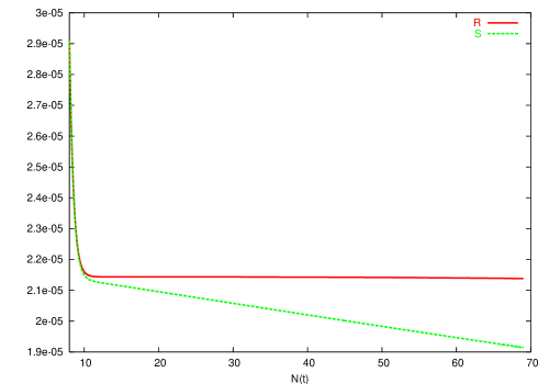
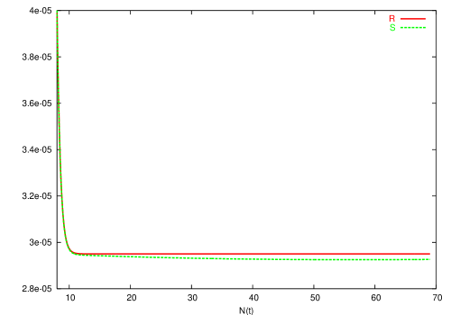
Refer to captionRefer to caption

Figure 2: Evolution of {\mathcal{R}} and 𝒮𝒮{\mathcal{S}} for a wavelength that leaves the horizon, N=8subscript𝑁8N_{*}=8, 60 e–folds before the end of inflation. The left figure shows the case β1=0.05subscript𝛽10.05\beta_{1}=0.05, β2=0.10subscript𝛽20.10\beta_{2}=0.10, m1=m2=1subscript𝑚1subscript𝑚21m_{1}=m_{2}=1, V0=1010subscript𝑉0superscript1010V_{0}=10^{-10} with initial conditions ϕ0=1,χ0=1formulae-sequencesubscriptitalic-ϕ01subscript𝜒01\phi_{0}=1,\chi_{0}=1. On the right hand side we now set m1=0.3subscript𝑚10.3m_{1}=0.3 leaving the other parameters unchanged. The plots show |P|12superscriptsubscript𝑃12|P_{\mathcal{R}}|^{\frac{1}{2}} and |P𝒮|12superscriptsubscript𝑃𝒮12|P_{\mathcal{S}}|^{\frac{1}{2}}.

Let us now observe how the spectral indices behave for all of parameter space. We set β1=0.05,β2=0.10formulae-sequencesubscript𝛽10.05subscript𝛽20.10\beta_{1}=0.05,\beta_{2}=0.10 and vary the powers m1,m2subscript𝑚1subscript𝑚2m_{1},m_{2}. We maintain the initial conditions ϕ0=1,χ0=1formulae-sequencesubscriptitalic-ϕ01subscript𝜒01\phi_{0}=1,\chi_{0}=1. The results are summarized in Figure 3. We find that n𝒞subscript𝑛𝒞n_{\mathcal{C}} always runs significantly so we do not include it here.
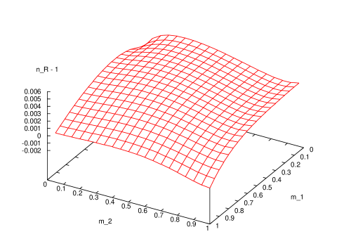
Refer to captionRefer to caption

Refer to captionRefer to caption

Refer to captionRefer to caption

Figure 3: Properties of the spectra for two exponentials. We set β1=0.05,β2=0.10formulae-sequencesubscript𝛽10.05subscript𝛽20.10\beta_{1}=0.05,\beta_{2}=0.10 and vary the powers m1,m2subscript𝑚1subscript𝑚2m_{1},m_{2} and we maintain the initial conditions ϕ0=1,χ0=1formulae-sequencesubscriptitalic-ϕ01subscript𝜒01\phi_{0}=1,\chi_{0}=1. All quantities are defined in the text. We remind the reader that the scale of P𝒮subscript𝑃𝒮P_{\mathcal{S}} is in general arbitrary but here it is equal to Psubscript𝑃P_{\mathcal{R}} at horizon crossing.

We observe in Figure 3 that the spectrum for the tensor modes is flat– to the extent that is indistinguishable from a flat spectrum with present observations– and the amount of tensor production is very small. Again this is below the level of current experiments. In general, the spectral indices are functions of the slow–roll parameters which decrease in time with run–away potentials. Thus the more inflation we allow the smaller the indices will be and the closer to scale invariance we will be. In fact, in all cases we can get arbitrarily close to a Harrison–Zel’dovich spectrum by allowing an arbitrarily large amount of inflation. Furthermore, one may expect the plots to be symmetric but we remind the reader that β1β2subscript𝛽1subscript𝛽2\beta_{1}\neq\beta_{2} so the two fields always have different potentials. Our results do not completely agree with the analytic results given above. The reason is that we have not yet reached the attractor solution for two exponential potentials. However, we have verified that once we are on the attractor, the analytic and numerical results agree sufficiently.

V.2.2 Two Inverse Power Potentials

To gain further insight here, it is helpful to use the field re–definition, eψ=χαsuperscript𝑒𝜓superscript𝜒𝛼e^{-\psi}=\chi^{-\alpha}. Then,

ψ=12α2e2αψ(ψ)2+V0χeψ.subscript𝜓12superscript𝛼2superscript𝑒2𝛼𝜓superscript𝜓2subscript𝑉subscript0𝜒superscript𝑒𝜓\displaystyle{\cal{L}}_{\psi}=\frac{1}{2\alpha^{2}}e^{\frac{2}{\alpha}\psi}(\partial\psi)^{2}+V_{0_{\chi}}e^{-\psi}. (172)

Therefore, this case corresponds to two scalar fields with non–canonical kinetic term and exponential potential. Because the non–canonical kinetic terms are a source of entropy perturbations, we expect that the entropy perturbations to be more strongly sourced when compared with the previous example of two straight exponentials. The data are shown in Figure 4.
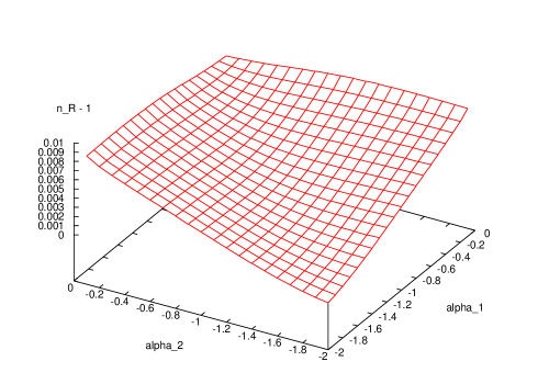
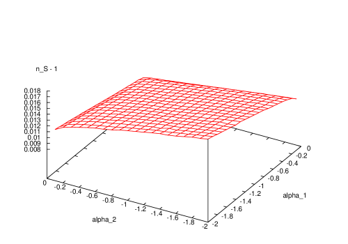
Refer to captionRefer to caption

Refer to captionRefer to caption

Refer to captionRefer to caption

Figure 4: Properties of the spectra for two inverse power potentials. We vary the powers α1,α2subscript𝛼1subscript𝛼2\alpha_{1},\alpha_{2} and we maintain the initial conditions ϕ0=1,χ0=1formulae-sequencesubscriptitalic-ϕ01subscript𝜒01\phi_{0}=1,\chi_{0}=1. All quantities are defined in the text. We remind the reader that the scale of P𝒮subscript𝑃𝒮P_{\mathcal{S}} is in general arbitrary but here it is equal to Psubscript𝑃P_{\mathcal{R}} at horizon crossing.

Compared with the case of two exponential potentials, the contribution of the entropy to the total perturbation is larger, but we see that the entropy modes are always smaller in magnitude than the curvature perturbation. Furthermore, adiabatic and isocurvature perturbations are effectively uncorrelated. The cleft in the plot arises from the background fields having the same evolution as they each have the same α𝛼\alpha. It is the clear that from our definition of P𝒞subscript𝑃𝒞P_{\mathcal{C}} that this quantity should be almost zero in this cleft. Once more the spectral index of the tenors is very small.

V.2.3 Mixed Case

We now consider the case of one field having an inverse power potential and the other an exponential potential. Again, we can transform the inverse power law potential into a exponential potential. It is then clear from the discussion of the last two subsections that the results for the spectra must be similar, as one can observe in Figure 5.
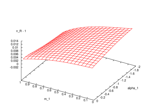
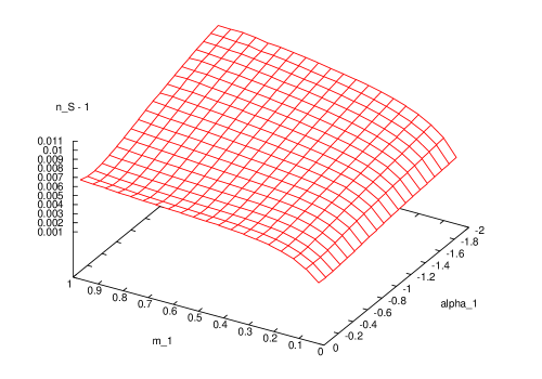
Refer to captionRefer to caption

Refer to captionRefer to caption

Refer to captionRefer to caption

Figure 5: Properties of the spectra for the mixed potential. We set β1=0.05subscript𝛽10.05\beta_{1}=0.05 and vary the powers m1,α2subscript𝑚1subscript𝛼2m_{1},\alpha_{2} . We maintain the initial conditions ϕ0=1,χ0=1formulae-sequencesubscriptitalic-ϕ01subscript𝜒01\phi_{0}=1,\chi_{0}=1. All quantities are defined in the text. We remind the reader that the scale of P𝒮subscript𝑃𝒮P_{\mathcal{S}} is in general arbitrary but here it is equal to Psubscript𝑃P_{\mathcal{R}} at horizon crossing.

V.2.4 Coupled Potential

Once more the features observed here are very similar to the cases studied so far. We set β=0.05𝛽0.05\beta=0.05 and vary the other parameters. The data are shown in Figures 6.
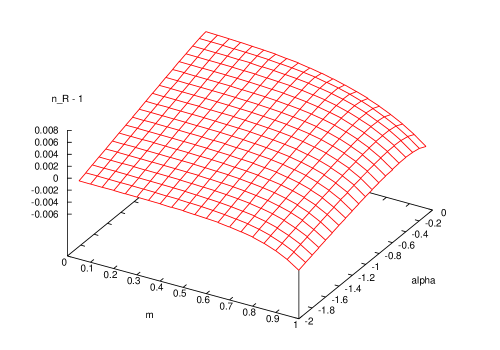
Refer to captionRefer to caption

Refer to captionRefer to caption

Refer to captionRefer to caption

Figure 6: Properties of the spectra for the coupled potential. We set β=0.05𝛽0.05\beta=0.05, vary the powers m,α𝑚𝛼m,\alpha and we maintain the initial conditions ϕ0=1,χ0=1formulae-sequencesubscriptitalic-ϕ01subscript𝜒01\phi_{0}=1,\chi_{0}=1. All quantities are defined in the text. We remind the reader that the scale of P𝒮subscript𝑃𝒮P_{\mathcal{S}} is in general arbitrary but here it is equal to Psubscript𝑃P_{\mathcal{R}} at horizon crossing.

V.2.5 Compatibility with WMAP

In general, all our models generate almost scale–invariant spectra with minimal tensor production. This also allows both red and blue spectra as seen in Figure 7. Furthermore, we are able to get arbitrarily close to scale–invariance by allowing more inflation. In addition, we find that the perturbations produced are essentially uncorrelated.

Let us comment on the compatibility with current experiments. The WMAP results have provided strong constraints on the initial power spectrum and hence on inflationary models wmap . If one examines Figure 7 one sees that it possible to have

0.9n1.3at 2σ.formulae-sequence0.9subscript𝑛1.3at2𝜎\displaystyle 0.9\leq n_{\mathcal{R}}\leq 1.3\ \ \mathrm{at}\ \ 2\sigma. (173)

We include the equivalent plot for our models.

Refer to captionRefer to caption

Figure 7: Allowed region for curvature index from the WMAP data alone. We scale our tensor/scalar ratio to agree with the WMAP team’s plot.One can clearly see the degeneracy in the predictions of r𝒯subscript𝑟𝒯r_{\mathcal{T}} and nsubscript𝑛n_{\mathcal{R}} among the possible models. For example as m0𝑚0m\rightarrow 0 in the coupled case we approach the results of the inverse power potential with the same dominant α𝛼\alpha. This is what we would have expected from the background solutions of sections 3 and 4.

One open issue we have not discussed is the end inflation. This may be caused by another scalar field. This process is, in general, non–adiabatic and would generate further entropy production which would add to that from the two fields. Hence, the spectra deep in the radiation dominated epoch depend on the details of reheating. Without a detailed study of this mechanism it is impossible to draw firm conclusions from the entropic values in all cases.

VI Conclusions

In this paper we have studied in considerable depth inflationary solutions generated by two scalar fields and potentials of the form V=V0ϕαexp(βϕm)𝑉subscript𝑉0superscriptitalic-ϕ𝛼𝛽superscriptitalic-ϕ𝑚V=V_{0}\phi^{-\alpha}\exp(-\beta\phi^{m}). This potential is very general and encompasses potentials motivated by supergravity and string theory and more general theories motivated by higher–dimensional gravity.

We have seen that it is possible to generate a large range of different inflating universes by varying the parameters in the theory. We find that slow–roll is a valid approximation by means of numerical calculations and we are able to verify that the analytic solutions presented in this paper hold. For two uncoupled fields (Section 3), we found that, often, only one of the fields is dominant. However, we also found solutions where both fields are important for the inflationary dynamics. For two coupled fields with the above potential (Section 4), we have found that only one of the fields dominates inflation, whereas the other field is only a background field. This case might be interesting if the background field acted as a curvaton field, for example.

We have used some of the background solutions we found to describe the evolution of the perturbations in two specific cases and, potentially, one would be able to find the transfer functions for all the solutions discussed here. We have demonstrated this with two examples. In general, however, one has to resort to numerical methods in order to evaluate the transfer functions. The solutions presented here thus allow one to make predictions about the relative size of \mathcal{R} and 𝒮𝒮\mathcal{S} for a large class of inflationary scenarios.

We made use of numerical calculations to investigate consequences for cosmological perturbations. We discussed the case where both fields contribute approximately equally to the expansion rate during a period of slow–roll inflation. We found that our models produce scale–invariant spectra with a small scalar–tensor ratio. By varying the parameters of the potential, it is possible to produce both red and blue spectra for the curvature perturbation. This is still consistent with observational constraints. Although the exact details depend on the initial condition of the fields, we don not expect our conclusions will be changed qualitatively. In the case of double inflation, one can generate uncorrelated polarski ,polarski2 as well as correlated perturbations, langlois . In contrast, in multi–field inflationary models with run–away potentials, the perturbations are always uncorrelated.

In order to make predictions for the anisotropies in the cosmic microwave background radiation, one has to follow the perturbations into the radiation dominated era, which involves a detailed calculation of the decay of both fields. Ending inflation in the class of models discussed here will involve presumably a third field, which becomes important just at the end of the inflationary stage.

In future work we will use some of these insights gained in this work in order study inflationary models in models with extra dimensions ashcroft .

Acknowledgements: We are grateful to H. Peiris and the other members of the WMAP team for Figure 7. The authors are supported in part by PPARC.

References

  • (1) A.R. Liddle, D. Lyth, Cosmological Inflation and Large Scale Structure, Cambridge University Press (2000)
  • (2) A. Riotto, hep-ph/0210162
  • (3) A. Linde, Phys.Rev.D 49, 748 (1994)
  • (4) L. Kofman, A. Linde, Nucl. Phys. B282, 555 (1987)
  • (5) D. Polarski, A.A. Starobinsky, Nucl.Phys.B 385, 623 (1992)
  • (6) D. Polarski, A.A. Starobinsky, Phys.Rev.D 50, 6123 (1994)
  • (7) J. Garcia-Bellido, D. Wands, Phys.Rev.D 53, 5437 (1996)
  • (8) C. Gordon, D. Wands, B.A. Bassett, R. Maartens, Phys.Rev.D 63, 023506 (2001)
  • (9) S. Groot Nibbelink, B.J.W. van Tent, Class.Quant.Grav. 19, 613 (2002)
  • (10) S. Tsujikawa, D. Parkinson, B. A. Bassett,Tsujikawa, Phys.Rev.D 67, 083516 (2003)
  • (11) N. Bartolo, S. Matarrese, A. Riotto, Phys.Rev. D64, 123504 (2001)
  • (12) D. Wands, N. Bartolo, S. Matarrese, A. Riotto, Phys.Rev.D 66, 043520 (2002)
  • (13) J.D. Barrow, Phys.Rev.D 48, 1585 (1993)
  • (14) P. Parsons, J.D. Barrow, Phys.Rev.D 51, 6757 (1995)
  • (15) P.G. Ferreira, M. Joyce, Phys.Rev.D 58, 023503 (1998)
  • (16) P. Binetruy, Phys.Rev.D 60, 063502 (1999)
  • (17) Ph. Brax, J. Martin, Phys.Lett.B 468, 40 (1999)
  • (18) T. Damour, F. Piazza, G. Veneziano, Phys.Rev.D. 66, 046007 (2002)
  • (19) P.J.E. Peebles, B. Ratra, Rev.Mod.Phys.75, 559 (2003)
  • (20) Ph. Brax, J. Martin, Phys.Rev.D 61, 103502 (2000)
  • (21) S.C.C. Ng, N.J. Nunes, F. Rosati, Phys.Rev.D 64, 083510 (2001)
  • (22) D.H. Lyth, D. Wands, Phys.Lett.B 524, 5 (2002)
  • (23) A.A. Coley, R.J. van den Hoogen, Phys. Rev.D 62, 023517 (2000)
  • (24) A.A. Starobinsky, S. Tsujikawa, J. Yokoyama, Nucl.Phys.B 610, 383 (2001)
  • (25) D. Wands, K. Malik, D. Lyth, A.R. Liddle, Phys.Rev.D 62, 043527 (2000)
  • (26) H. V. Peiris et al, Astrophys.J.Suppl. 148, 213 (2003)
  • (27) K. Malik, D. Wands, Phys.Rev.D 59, 123501 (1999)
  • (28) F. Di Marco, F. Finelli, R. Brandenberger, Phys.Rev.D 67, 063512 (2003)
  • (29) D. Langlois, Phys. Rev.D 59, 123512 (1999)
  • (30) P.R. Ashcroft, C. van de Bruck, A.-C. Davis, astro-ph/0310643