A New Search Technique for Short Orbital Period Binary Pulsars

Abstract

We describe a new and efficient technique which we call sideband or phase-modulation searching that allows one to detect short period binary pulsars in observations longer than the orbital period. The orbital motion of the pulsar during long observations effectively modulates the phase of the pulsar signal causing sidebands to appear around the pulsar spin frequency and its harmonics in the Fourier transform. For the majority of binary radio pulsars or Low-Mass X-ray Binaries (LMXBs), large numbers of sidebands are present, allowing efficient searches using Fourier transforms of short portions of the original power spectrum. Analysis of the complex amplitudes and phases of the sidebands can provide enough information to solve for the Keplerian orbital parameters. This technique is particularly applicable to radio pulsar searches in globular clusters and searches for coherent X-ray pulsations from LMXBs and is complementary to more standard “acceleration” searches.

1 Introduction

Short orbital-period binary pulsars have proven to be sensitive laboratories that allow tests of a variety of physical processes including theories of gravitation. Unfortunately, except for those systems containing the brightest pulsars, they are notoriously difficult to detect. When the observation time $T_{obs}$ is greater than a small fraction of the orbital period $P_{orb}$, Doppler effects due to the orbital motion of the pulsar cause drastic reductions in the sensitivities of pulsar searches (Johnston & Kulkarni 1991).

Numerous groups (e.g. Middleditch & Kristian 1984; Anderson et al. 1990; Wood et al. 1991) have developed variations of so called “acceleration” searches in order to mitigate the loss in sensitivity caused by orbital motion. These searches can almost completely recover this lost sensitivity when $T_{obs}\lesssim P_{orb}/10$ by taking advantage of the fact that orbital motion causes an approximately linear drift of the pulsar spin frequency $f_{spin}$. Recent acceleration searches of globular clusters have discovered numerous binary systems, some with orbital periods as short as $\sim 90$ min (Camilo et al. 2000; Ransom et al. 2001; D’Amico et al. 2001).

Acceleration searches are effective only for $T_{obs}\lesssim P_{orb}/10$, but search sensitivities improve as $T_{obs}^{1/2}$. In effect, acceleration searches are limited to discovering only the brightest binary pulsars in ultra-compact — systems with orbital periods less than a few hours — orbits. For a 2 ms pulsar in a 1 hour orbit with a low mass white dwarf (WD) companion, the optimal observation time $T_{best}$ for an acceleration search (using eqn. 22 from Johnston & Kulkarni 1991) is only $\sim 300-600$ seconds. If this pulsar were located in a globular cluster, where observations of $5-10$ hours in duration are common, acceleration searches would be a factor of $\sqrt{T_{obs}/T_{best}}\sim 8$ times less sensitive than an optimal (i.e. coherent) search of a full observation.

We have developed an efficient search technique for short orbital period binary pulsars that complements the use of acceleration searches. Since it requires $T_{obs}\gtrsim 1.5P_{orb}$ and its sensitivity improves as the ratio $r_{orb}=T_{obs}/P_{orb}$ increases, it allows the search of very interesting portions of orbital parameter space for the first time. This technique was developed and tested over the past several years as part of a Ph.D. thesis (Ransom 2001). A similar but independent derivation of many of the properties of this technique has been recently published by Jouteux et al. (2002), based on an earlier mention of this work in Ransom (2000). While the basic search techniques presented by these papers are nearly identical, aspects concerning the determination of the orbital elements of a candidate pulsar discovered with this technique are presented in more detail in this work.

2 Phase Modulation due to Orbital Motion

During observations of a binary pulsar where $T_{obs}$ is longer than $P_{orb}$, the orbital motion causes a modulation of the phase of the pulsar signal. Differences in light travel time across the projected orbit advance or delay the pulse phase in a periodic fashion.

2.1 Circular Orbits

If the orbit is circular (where the eccentricity $e$ and the angle of periapsis $\omega$ are both zero), the phase delays are sinusoidal. The fundamental harmonic of the resulting signal as sampled at a telescope can be described by

$$n_{j}=n(u)=a\,\cos\left[2\pi r_{spin}u+\phi_{spin}+\Phi_{orb}\cos(2\pi r_{orb}u+\phi_{orb})\right],$$ (1)

where $a$ and $\phi_{spin}$ are the amplitude and phase of the pulsation, $\Phi_{orb}$ and $\phi_{orb}$ are the amplitude and phase of the modulation due to the orbit, $r$ is a Fourier frequency (i.e. $r=fT_{obs}=T_{obs}/P$), and $u=j/N=(t_{j}-t_{o})/T_{obs}$ is the discrete dimensionless time during the observation of the $j^{th}$ sample of $N$ such that $0\leq u\leq 1$. We can write $\Phi_{orb}$ and $\phi_{orb}$ in terms of the three Keplerian orbital parameters for circular orbits ($P_{orb}$, the semi-major axis $x_{orb}=a_{1}\sin(i)/c$, and the time of periapsis $T_{o}$) as

$$\Phi_{orb}=2\pi x_{orb}f_{spin}\simeq 7.375\,\frac{f_{1}^{1/3}P_{orb}^{2/3}({\rm hr})}{P_{spin}({\rm sec})}$$ (2)

and

$$\phi_{orb}=2\pi\frac{t_{o}-T_{o}}{P_{orb}}+\frac{\pi}{2},$$ (3)

where the units of both are radians, and the pulsar’s mass function $f_{1}$ is defined as

$$f_{1}=\frac{\left[M_{2}\sin(i)\right]^{3}}{\left(M_{1}+M_{2}\right)^{2}},$$ (4)

where $i$ is the orbital inclination and $M_{1}$ and $M_{2}$ are the pulsar and companion masses (in solar masses) respectfully.

The Discrete Fourier Transform (DFT) of the signal in eqn. 1 when $\Phi_{orb}=0$ can be approximated as (see e.g.  Ransom, Eikenberry, & Middleditch 2002)

$$A(r) = \sum_{j=0}^{N-1}n_{j}\,\mathrm{e}^{-2\pi\mathrm{i}jr/N}\simeq N\int_{0}^{1}n(u)\,\mathrm{e}^{-2\pi\mathrm{i}ru}\,\mathrm{d}u$$ (5a)

$$\simeq \frac{aN}{2}\,\mathrm{e}^{\mathrm{i}\phi_{spin}}\int^{1}_{0}\mathrm{e}^{2\pi\mathrm{i}(r_{spin}-r)u}\,\mathrm{d}u$$ (5b)

$$= A_{coherent}\,\mathrm{e}^{\mathrm{i}\pi(r_{spin}-r)}\frac{\sin\left[\pi(r_{spin}-r)\right]}{\pi(r_{spin}-r)},$$ (5c)

where $A_{coherent}=\frac{aN}{2}\,\mathrm{e}^{\mathrm{i}\phi_{spin}}$ represents the coherent Fourier response at the spin frequency $r_{spin}$. Similarly, we can approximate the DFT of our phase modulated signal from eqn. 1 as

$$A(r) = \frac{aN}{2}\int^{1}_{0}\mathrm{e}^{\mathrm{i}\left[2\pi r_{spin}u+\phi_{spin}+\Phi_{orb}\cos(2\pi r_{orb}u+\phi_{orb})\right]}\,\mathrm{e}^{-2\pi\mathrm{i}ru}\,\mathrm{d}u$$ (6a)

$$= A_{coherent}\int^{1}_{0}\mathrm{e}^{\mathrm{i}\Phi_{orb}\cos(2\pi r_{orb}u+\phi_{orb})}\,\mathrm{e}^{2\pi\mathrm{i}(r_{spin}-r)u}\,\mathrm{d}u.$$ (6b)

Using the Jacobi-Anger expansion (e.g. Arfken 1985)

$$\mathrm{e}^{\mathrm{i}z\cos(\theta)}=\sum_{m=-\infty}^{\infty}\mathrm{i}^{m}J_{m}(z)\,\mathrm{e}^{\mathrm{i}m\theta}=\sum_{m=-\infty}^{\infty}J_{m}(z)\,\mathrm{e}^{\mathrm{i}m\left(\theta+\frac{\pi}{2}\right)},$$ (7)

where $J_{m}(z)$ is an integer order Bessel function of the first kind, we can expand the integrand in eqn. 6b to give

$$A(r) = A_{coherent}\sum_{m=-\infty}^{\infty}J_{m}(\Phi_{orb})\int^{1}_{0}\mathrm{e}^{\mathrm{i}m(2\pi r_{orb}u+\phi_{orb}+\frac{\pi}{2})}\,\mathrm{e}^{2\pi\mathrm{i}(r_{spin}-r)u}\,\mathrm{d}u$$ (8a)

$$= A_{coherent}\sum_{m=-\infty}^{\infty}J_{m}(\Phi_{orb})\,\mathrm{e}^{\mathrm{i}m\left(\phi_{orb}+\frac{\pi}{2}\right)}\int^{1}_{0}\mathrm{e}^{2\pi\mathrm{i}\left(r_{spin}+mr_{orb}-r\right)u}\,\mathrm{d}u.$$ (8b)

Since the integrand in eqn. 8b is identical in form to that in eqn. 5b, the Fourier transform of a phase modulated signal is equivalent to the Fourier transform of a series of cosinusoids at frequencies centered on the pulsar spin frequency $r_{spin}$, but separated from $r_{spin}$ by $mr_{orb}$ Fourier bins (i.e. sidebands). The response is therefore

$$A(r)=A_{coherent}\sum_{m=-\infty}^{\infty}J_{m}(\Phi_{orb})\,\mathrm{e}^{\mathrm{i}m\left(\phi_{orb}+\frac{\pi}{2}\right)}\,\mathrm{e}^{\mathrm{i}\pi(r_{spin}+mr_{orb}-r)}\,\frac{\sin\left[\pi(r_{spin}+mr_{orb}-r)\right]}{\pi(r_{spin}+mr_{orb}-r)}.$$ (9)

When $r_{orb}$ is an integer (i.e. the observation covers an integer number of complete orbits), the Fourier response shown in eqn. 9 becomes particularly simple at Fourier frequencies $r_{spin}+sr_{orb}$, where $s$ is an integer describing the sideband in question. In this case, the summation collapses to a single term when $m=s$, giving

$$A\left(r_{spin}+sr_{orb}\right)=A_{coherent}J_{s}(\Phi_{orb})\,\mathrm{e}^{\mathrm{i}s\left(\phi_{orb}+\frac{\pi}{2}\right)}.$$ (10)

In effect, the phase modulated signal produces sidebands composed of a series of sidebands split in frequency from $r_{spin}$ by $sr_{orb}$ Fourier bins, with amplitudes proportional to $J_{s}(\Phi_{orb})$, and phases of $s\left(\phi_{orb}+\frac{\pi}{2}\right)+\phi_{spin}$ radians. Figure 1 shows the Fourier response for a “typical” pulsar-WD system in a circular 50 min orbit during an 8 hour observation.

While the number of sidebands implied by eqn. 9 is infinite (assuming $\Phi_{orb}\neq 0$), properties of the Bessel functions — which define the magnitude of the Fourier amplitudes of the sidebands — give a rather sharp cutoff at $\sim 2\Phi_{orb}$ sidebands (or $\sim\Phi_{orb}$ pairs of sidebands). The maximum value of $J_{s}(\Phi_{orb})$ also occurs near $s=\Phi_{orb}$ at a value of $\sim 0.675\Phi_{orb}^{-1/3}$, which gives the phase modulation response its distinctive “horned” shape when $\Phi_{orb}$ is large (see Fig. 1). The average magnitude of the phase modulation sidebands falls off more quickly as $\sim 0.611\Phi_{orb}^{-1/2}$ (see Fig. 2).

For pulsars with narrow pulse shapes and many Fourier harmonics, phase modulation produces sidebands split by $r_{orb}$ Fourier bins centered around each spin harmonic. For spin harmonic number $h$, the phase modulation amplitude is $\Phi_{orb,h}=2\pi x_{orb}hf_{spin}$. Therefore, for large $\Phi_{orb,h}$, there are $\sim h$ times more sidebands than around the fundamental, but the average amplitudes are smaller by a factor of $\sim h^{-1/2}$.

2.2 Small Amplitude Limit

When $\Phi_{orb}\ll 1$, a phase modulated signal will have only three significant peaks in its Fourier response. These peaks are located at $r_{spin}$ and $r_{spin}\pm r_{orb}$ and have magnitudes proportional to $J_{0}(\Phi_{orb})\sim 1-\Phi_{orb}^{2}/4\sim 1$ and $J_{\pm 1}(\Phi_{orb})\sim\pm\Phi_{orb}/2$ respectively.

Middleditch et al. (1981) performed a detailed analysis of phase modulated optical pulsations in the small amplitude limit from the 7.7 second X-ray pulsar 4U 1626-67 in order to solve for the orbital parameters of the system. The separation of the sidebands provided a measurement of the $\sim 42$ min orbital period and the magnitudes and phases of the three significant Fourier peaks allowed them to solve for $\Phi_{orb}$ (and therefore $x_{orb}$) and $\phi_{orb}$ directly.

Small amplitude phase modulation might also be observed from freely precessing neutron stars (e.g. Nelson, Finn, & Wasserman 1990; Glendenning 1995). For certain geometries, the geometric wobble of the pulsar beam would periodically modulate the pulse arrival times and cause the system to appear as a compact binary. If such rapidly precessing objects exist, they would display a small number ($\sim 1-3$) of pairs of sidebands in a power spectrum of a long observation, since the maximum possible phase modulation amplitude for such a system is $\Phi_{orb}\lesssim\pi/2$ radians (Nelson et al. 1990).

2.3 Elliptical Orbits

Konacki & Maciejewski (1996) derived a Fourier expansion for elliptical orbital motion with the useful property that the magnitudes of higher order harmonics of the orbital expansion (which correspond to independent modulation amplitudes $\Phi_{orb,h^{\prime}}$) decrease monotonically. In the limit of circular orbits the expansion reduces to the single phase modulating sinusoid found in eqn. 1.

Each harmonic of the orbital modulation generates sidebands around the spin harmonic of the form discussed in §2.1. The sidebands created by harmonic $h^{\prime}$ of the orbital expansion are separated from each other by $h^{\prime}r_{orb}$ Fourier bins. Since $\Phi_{orb,h^{\prime}}$ monotonically decreases with increasing orbital harmonic $h^{\prime}$, the number of sidebands generated decreases while their spacing and average amplitudes increase. The most important aspect of this superposition of sidebands is the fact that the Fourier response near a spin harmonic contains sidebands spaced by $r_{orb}$ Fourier bins — from the fundamental of the orbital expansion — just as in the limiting case of circular orbits.

3 Pulsars with Deterministic Periodic Phase Modulation

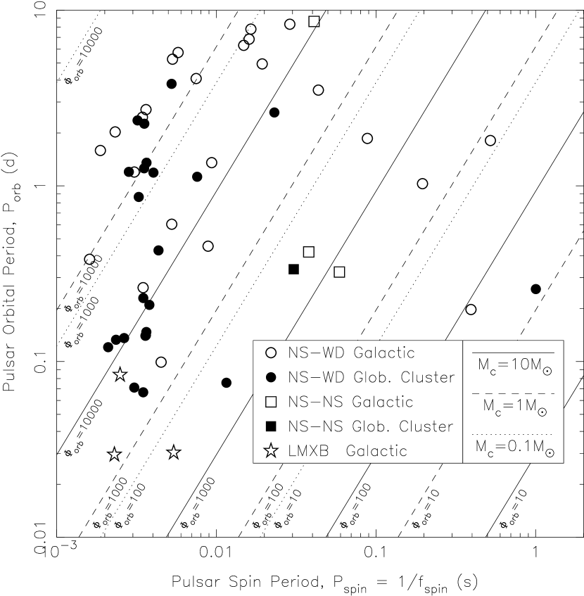
Figure 3: Orbital versus spin periods for 54 currently known binary pulsars with $P_{orb}<10$ d. The symbols denote the type of system (circles for NS-WD systems, squares for NS-NS systems, and stars for the three recently discovered accreting X-ray MSPs) as well as its location in the galaxy or a globular cluster (open or filled respectively). Lines of constant phase modulation amplitude $\Phi_{orb}=2\pi x_{orb}f_{spin}$ are overlaid assuming orbital inclinations of 60°, pulsar masses of 1.4 $\mbox{M}_{\odot}$, and companion masses of 0.1, 1, and 10 $\mbox{M}_{\odot}$ for dotted, dashed, and solid lines respectively.

Figures 3 and 4 show $P_{spin}$, $P_{orb}$, and $\Phi_{orb}$ for 54 binary pulsars from the literature, all with orbital periods less than 10 days. A few conclusions can be reached immediately. First, radio millisecond pulsars (MSPs) are the most common binary pulsar. Second, there is a relatively flat distribution of $P_{orb}$ for radio pulsars which cuts off quite dramatically near $P_{orb}\sim 0.08$ d ($\sim 2$ h) — the two systems with shorter orbital periods are the recently discovered accreting X-ray MSPs XTE J1751-314 (Markwardt et al. 2002) and XTE J0929-314 (Galloway et al. 2002). And third, a large fraction of the systems are located in globular clusters.

The fact that large numbers of relatively compact binary pulsar systems should contain MSPs is not surprising in light of the standard “recycling” model for MSP creation (Verbunt 1993; Phinney & Kulkarni 1994). This model explains not only the preponderance of pulsars with millisecond spin periods, but also the fact that many MSPs have low-mass ($\sim 0.02-0.4\,\mbox{M}_{\odot}$) companion stars in compact circular orbits. These recycled systems make up the vast majority of the pulsars shown in Figure 3 and have typical values of $\Phi_{orb}$ of $10^{2}$ to a few times $10^{3}$ radians.

The cutoff in $P_{orb}$ at approximately two hours is almost certainly due in some part to selection effects. The rapid orbital motion of these systems prevents their detection using conventional search techniques — including acceleration searches — for all but the brightest systems (Johnston & Kulkarni 1991). In fact, the only MSPs discovered with shorter orbital periods ($P_{orb}\sim 40$ min for both XTE J1751-314 and XTE J0929-314) were discovered during transient X-ray outbursts when the pulsed fractions were very high (Markwardt et al. 2002; Galloway et al. 2002). Since selection effects keep us from detecting ultra-compact systems that are not exceptionally bright, it is difficult to determine how much the observed lack of such systems is due to a true lack of compact systems. It is certain that neutron star (NS) systems with much shorter orbital periods do exist, as the new accreting X-ray MSPs and other ultra-compact LMXBs such as 4U 1820$-$303 ($P_{orb}\sim 11$ min), 4U 1850$-$087 ($P_{orb}\sim 21$ min), 4U 1627$-$673 ($P_{orb}\sim 42$ min), and 4U 1916$-$053 ($P_{orb}\sim 50$ min) (Chou et al. 2001; Liu et al. 2001) have shown.

The large fraction of known systems inhabiting globular clusters can be explained by three basic facts. First, due to their known location on the sky, long targeted observations of clusters allow fainter systems to be detected (e.g. Anderson 1992). Second, repeated observations of certain clusters have allowed many very weak pulsars to be detected with the help of amplification from interstellar scintillation (Camilo et al. 2000; Possenti et al. 2001). Finally, large numbers of binary pulsars are expected to have been created in globular clusters due to dynamical interactions (e.g. Kulkarni & Anderson 1996; Davies & Hansen 1998; Rasio et al. 2000).

Recently, Rasio et al. (2000) have conducted extensive population synthesis studies for binary pulsars in dense globular clusters like 47 Tucanae. Their initial results imply that exchange interactions among primordial binaries will produce large numbers of NSs in binary systems. In fact, their results predict that large populations of binary pulsars with low mass companions ($m_{c}\sim 0.05\,\mbox{M}_{\odot}$) should exist in many globular clusters with orbital periods as short as $\sim 15$ min.

The evidence seems to suggest that a large population of ultra-compact binary pulsars should exist — particularly in globular clusters — which have so far eluded detection. With long observations, these pulsars will be detected if search algorithms can identify the distinctive sidebands generated by the systems. The rest of this paper discusses such an algorithm.

4 Sideband Searches

The fact that power from an orbitally modulated sinusoid is split into multiple sidebands allows us to increase the signal-to-noise of the detected response by incoherently summing the sidebands. According to one of the addition theorems of Bessel functions

$$\sum_{m=-\infty}^{\infty}J_{m}(z)^{2}=1,$$ (11)

theoretically all of the signal power can be recovered in this manner for noiseless data. Practically, though, complete recovery of signal power is not possible for data with a finite signal-to-noise ratio — especially if $\Phi_{orb}\gg 1$. Such a summation would require calculation of the $\sim 2\Phi_{orb}$ significant sidebands at the precise Fourier frequencies of their peaks $r_{spin}\pm sr_{orb}$. This computationally daunting task would result in very large numbers of independent search trials when $\Phi_{orb}$, $r_{spin}$, and $r_{orb}$ are unknown.

Even if we could recover all of the power using a sum of the sidebands, the significance of the measurement would be less than the significance of a non-modulated sinusoid with the same Fourier power. This loss in significance is due to the fact that noise is co-added along with signal. The exact loss in significance can easily be calculated since the probability for a sum of $m$ noise powers to exceed some power $P_{sum}$ is the probability for a $\chi^{2}$ distribution of $2m$ degrees of freedom to exceed $2P_{sum}$ (see e.g. Groth 1975, and references therein).

In the case where only a few sidebands are suspected to be present (i.e. $\Phi_{orb}\lesssim 5$), a brute-force search using incoherent sideband summing may be computationally feasible and worthwhile. Unfortunately, except for binary X-ray pulsars with long spin periods and possibly certain freely precessing NSs (see §2.2), the number of astrophysical systems with $\Phi_{orb}\lesssim 5$ is probably small compared to those with $\Phi_{orb}\gg 1$ (see §3).

4.1 Two-Staged Fourier Analysis

For systems with $\Phi_{orb}\gg 1$, the large number of regularly spaced sidebands allows a very efficient detection scheme. Since the sidebands are separated from each other by $r_{orb}$ Fourier bins, they appear as a localized periodicity in the power spectrum of the original time series which can be detected with a second stage of Fourier analysis. By stepping through the full length power spectrum and taking short Fast Fourier Transforms (FFTs) of the powers, we incoherently sum any sidebands present and efficiently detect their periodic nature. As an added benefit, the measured “frequency” of these “sideband pulsations” gives a direct and accurate measurement of the orbital period.

We define the following notation to represent the two distinct stages of the Fourier analysis for detecting a phase modulated signal. As defined in eqn. 1, the initial time series $n_{j}$ contains $N$ points. After Fourier transforming the $n_{j}$ (usually using an FFT of length $N$), the complex responses at Fourier frequencies $r$ are represented by $A(r)$ as defined in eqn. 5a. The powers and phases are then simply $P(r)$ and $\phi(r)$ respectively. The short FFTs of the $P(r)$ used to detect the sideband pulsations (i.e. the secondary power spectrum) are of length $M$ (where $M\ll N$ and should closely match the extent of the sideband structure in the original power spectrum) and generate complex responses $A_{2}(r)$, powers $P_{2}(r)$, and phases $\phi_{2}(r)$.

In order for a pulsed signal to undergo enough modulation to produce periodic sidebands, the observation must contain more than one complete orbit (i.e. $r_{orb}>1$). One might initially think that two complete orbits would be necessary to create a Nyquist sampled series of sidebands in the original power spectrum. However, since the sideband pulsations are not bandwidth limited, periodic signals with “wavelengths” less than two Fourier bins (i.e. $r_{orb}<2$) will still appear in the $P_{2}(r)$. Instead of appearing at Fourier frequency $r=M/r_{orb}$ as for signals with $r_{orb}>2$ (see §4.2.2), the fundamental harmonic of the response will appear aliased around the Nyquist frequency ($r_{Nyq}=M/2$) at $r_{alias}=M-M/r_{orb}$. While $r_{orb}>1$ is required to begin to produce periodic sidebands, simulations have shown that this technique realistically requires $r_{orb}\gtrsim 1.5$ to create detectable sidebands from most binary systems during reasonable observations.

As the number of orbits present in the data ($r_{orb}$) increases, so does the spacing (in Fourier bins) between the sidebands. Since each sideband has a traditional sinc function shape in $A_{2}(r)$ (see §2.1), the full-width at half-maximum (FWHM) of a sideband is approximately one Fourier bin. Therefore, an increase in spacing effectively decreases the duty-cycle of the sideband pulsations (i.e. $\sim 1/r_{orb}$). Signals with small duty-cycles are easier to detect for two reasons. First, significant higher harmonics begin to appear in $P_{2}(r)$ which can be incoherently summed in order to improve the signal-to-noise ratio. A rule-of-thumb for the number of higher harmonics present in $P_{2}(r)$ is approximately one-half the inverse of the duty-cycle ($\sim r_{orb}/2$). Second, as the duty-cycle decreases, the Fourier amplitudes of each harmonic increase in magnitude up to a maximum of twice that of a sinusoid with an identical pulsed fraction (see Ransom et al. 2002, for a more detailed discussion of pulse duty-cycle effects). This effect makes each individual harmonic easier to detect as $r_{orb}$ increases.

4.2 Search Considerations

As the number of orbits present in a time series increases, the signal-to-noise ratio of a detectable pulsar spin harmonic goes approximately as $\sim(r_{orb}-1)^{-\beta}$ where $0.3\lesssim\beta\lesssim 0.4$ (see Figures 6 and 7). In contrast, the signal-to-noise ratio of a pulsar spin harmonic detected coherently goes as $T_{obs}^{-1/2}$. This leads to a rule-of-thumb for those conducting sideband searches: “The longer the observation the better.” When making very long observations it is important to keep the on-source time (i.e. the window function) as continuous and uniform as possible. Significant gaps in the data — especially periodic or recurring gaps of the kind common in X-ray observations — create side-lobes around Fourier peaks of constant-frequency pulsations that a sideband search will detect. It is a good idea before a sideband search to take the power spectrum of the power spectrum of the known window function in order to identify spurious orbital periods that a sideband search might uncover.

Since phase modulation sidebands require coherent pulsations (i.e. $f_{spin}$ is constant in time) in order to form, it may be necessary to correct the time series (or equivalently the Fourier transform) such that the underlying pulsations are coherent. As an example, if the telescope’s motion with respect to the solar system barycenter is not taken into account during long observations, interstellar pulsations — and therefore any phase modulation sidebands as well — will be “smeared” across numerous Fourier bins due to Doppler effects. By stretching or compressing the time series to account for the Earth’s motion before Fourier transforming (or equivalently, by applying the appropriate Fourier domain matched filter after the Fourier transform, see Ransom et al. 2002) the smeared signal can be made coherent for the purposes of the sideband search.

If the time-dependence of $f_{spin}$ is unknown a priori, due to accretion in an LMXB, the spin-down of a young pulsar, or timing (spin) noise, for example, one could in principle attempt a series of trial corrections and a sideband search for each trial. Such a search methodology is similar in computational complexity to traditional “acceleration” searches.

While §4.1 provided basic principles for detecting compact binary pulsars using the two-staged Fourier analysis, in the rest of this section we provide a more detailed discussion of how a search might be conducted. Figure 5 shows two examples of sideband searches. The left column shows data from an 8 h observation of the globular cluster 47 Tucanae taken with the Parkes radio telescope at 20 cm on 2000 November 17. The signal is the fundamental harmonic of the 2.1 ms binary pulsar 47 Tuc J ($f_{spin}=476.05$ Hz, $P_{orb}=2.896$ h, $r_{orb}=2.762$, $\Phi_{orb}=120.87$ radians, and $m_{c}\sim 0.03$ $\mbox{M}_{\odot}$) with a signal-to-noise ratio of $\eta=a/\sigma_{n_{j}}\sim 0.0054$. The right column shows data from a simulated 8 h observation similar to the 47 Tuc observation described above. The signal is the fundamental harmonic of the 2.0 ms binary pulsar used in Figure 1 ($f_{spin}=500$ Hz, $P_{orb}=50$ min, $r_{orb}=8$, $\Phi_{orb}=413.44$ radians, and $m_{c}=0.2$ $\mbox{M}_{\odot}$) with a signal-to-noise ratio one half that of the 47 Tuc J observation ($\eta\sim 0.0027$).

Once a long observation has been obtained and prepared as discussed above, we Fourier transform the data and compute the power spectrum $P(r)$. We then begin a sideband search which is composed of two distinct parts: initial detection of a binary pulsar and the determination of a detected pulsar’s orbital elements.

4.2.1 Initial Detection

To maximize the signal-to-noise of a detection in $P_{2}(r)$, we want to match both the length and location of a short FFT $M$ with the width and location of a pulsar’s sideband response ($\sim 2r_{orb}\Phi_{orb}$) in $P(r)$. Because a pulsar’s orbital parameters are unknown a priori, we must search a range of short FFT lengths $M$ and overlap consecutive FFTs. Therefore, we must choose the number and lengths of the short FFTs, the fraction of each FFT to overlap with the next, and the number of harmonics to sum in each FFT. These choices are influenced by the length of the observation and the nature of the systems that we are attempting to find.

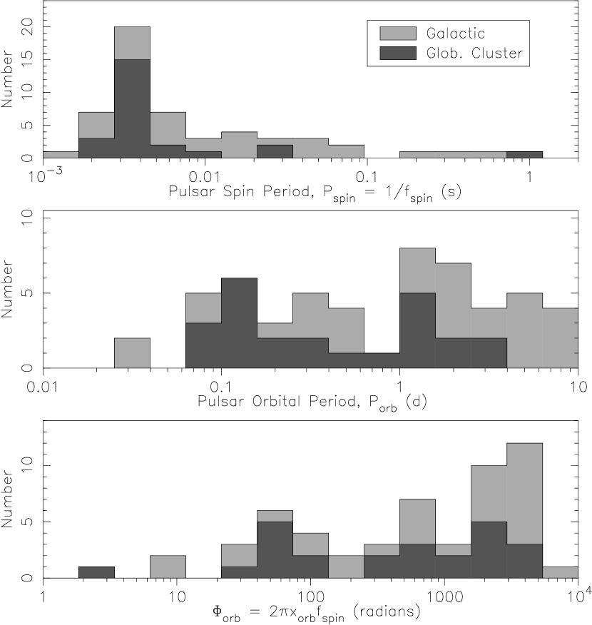
Figure 4: Histograms of spin period, orbital period, and phase modulation amplitude $\Phi_{orb}$ for the 54 binary pulsar systems described in Fig. 3.

All currently known binary pulsars with $P_{orb}<10$ d have modulation amplitudes of $\Phi_{orb}\lesssim 6500$ radians (see Figure 4), with the vast majority in the range $\Phi_{orb}\sim 20-5000$ radians. This range also includes many currently unknown but predicted “holy grail”-type systems such as compact MSP-black hole systems or MSP-WD systems with orbital periods of $\sim 10$ min. This range of $\Phi_{orb}$ values is due to the fact that the short spin periods of MSPs tend to offset the small semi-major axes ($x_{orb}$) of their typical binary systems, while binary systems with wider orbits tend to have longer spin periods. Multiplying this range by twice the minimum $r_{orb}$ of 1.5 gives a rule-of-thumb range of $M\sim 60-15000$ where the high end should be increased based on expected values of $r_{orb}$. For $8-12$ h globular cluster searches a reasonable range of values would be $64\lesssim M\lesssim 65536$ in powers-of-two increments, for a total of 11 different values for $M$.

The choice of the overlap fraction is more subjective. To optimize a detection in $P_{2}(r)$, one should overlap the short FFTs by at least 50% in order to avoid excessive loss of signal-to-noise when a series of sidebands straddles consecutive FFTs. Larger overlap percentages may result in higher signal-to-noise, but at the expense of increased computational costs and numbers of search trials (even though the trials are not completely independent when overlapping).

In Figure 5 plots $a$ and $e$, the grey shaded regions show the sections of the $P(r)$ that were Fourier transformed for the sideband search. The short FFTs of length $M=1024$ and $M=8192$ were centered on the known pulsar spin frequency and resulted in the $P_{2}(r)$ displayed in plots $b$ and $f$ respectively. The short FFT lengths were chosen as the shortest powers-of-two greater than $2r_{orb}\Phi_{orb}$. For 47 Tuc J (plot $a$), the “horned” structure of the phase modulation sidebands described in §2.1 is easily recognizable. This shape is not apparent in plot $e$, and in fact, traditional searches would detect nothing unusual about this section of the power spectrum.

Normalization of the $P_{2}(r)$ results in the usual exponential distribution with mean and standard deviation of one for a transform of pure noise. If one first normalizes the $P(r)$ as shown in plots $a$ and $e$ (see Ransom et al. 2002, for several normalization techniques), the resulting $P_{2}(r)$ can be normalized simply by dividing by $M$.

Plots $b$ and $f$ of Figure 5 show the highly significant detections of the binary pulsars in $P_{2}(r)$. For 47 Tuc J, only one orbital harmonic is visible in $P_{2}(r)$ since $r_{orb}<2$, but the single-trial significance is approximately $\sim 23\,\sigma$. For the simulated 50 min binary pulsar, 3 significant orbital harmonics are detected (predicted harmonic locations are marked with a dotted line in plot $f$). When summed, the detection has a single-trial significance of $\sim 15\,\sigma$.

4.2.2 Orbit Determination

Once a binary pulsar has been detected, examination of the $P(r)$ and $\phi(r)$ allow the estimation of the Keplerian orbital parameters and the pulsar spin period $P_{spin}$. Brute-force matched filtering searches centered on the estimates are then used to refine the parameters and recover the fully coherent response of the pulsar.

The simplest parameter to determine is the orbital period $P_{orb}$. The spacing between sidebands is $r_{orb}=T_{obs}/P_{orb}$ bins, implying that the most significant peak in $P_{2}(r)$ should occur at Fourier frequency $M/r_{orb}$. Conversely, if we measure the Fourier frequency $r_{meas}$ in $P_{2}(r)$ with the most power, we can solve for $r_{orb}$ using $r_{orb}=M/r_{meas}$. By using Fourier interpolation or zero-padding to oversample $A_{2}(r)$ and $P_{2}(r)$, we can determine $r_{meas}$ to an accuracy of

$$\sigma_{r}=\frac{3}{\pi\alpha\sqrt{6P_{2}(r_{meas})}},$$ (12)

where $P_{2}(r_{meas})$ is the normalized power at the peak and $\alpha$ is the signal “purity” — a property that is proportional to the root-mean-squared (RMS) dispersion of the pulsations in time about the centroid — which is equal to one for pulsations present throughout the data (see Middleditch et al. 1993; Ransom et al. 2002). Remembering that $P_{orb}=T_{obs}/r_{orb}$ and solving gives

$$P_{orb}=\frac{T_{obs}r_{meas}}{M}\pm\frac{3T_{obs}}{\pi\alpha M\sqrt{6P_{2}(r_{meas})}}.$$ (13)

For aliased signals, the orbital period is

$$P_{orb,aliased}=\frac{T_{obs}\left(M-r_{meas}\right)}{M}\pm\frac{3T_{obs}}{\pi\alpha M\sqrt{6P_{2}(r_{meas})}}.$$ (14)

For pulsars with $\Phi_{orb}\gg 1$ observed such that $r_{orb}>2$, it is often possible to measure $P_{orb}$ to one part in $10^{4}$, corresponding to a $\sim 1$ s error for many of the pulsars shown in Figure 4.

Once $P_{orb}$ is known it becomes possible to measure the projected semi-major axis $x_{orb}$ by determining the total width of the sidebands in $P(r)$. For bright pulsars like 47 Tuc J, the number of Fourier bins between the “horns” ($\Delta_{r}\sim 2\Phi_{orb}r_{orb}$) as shown in Figure 5$a$ can be measured directly and converted into $x_{orb}$ using

$$x_{orb}\simeq\frac{\Delta_{r}}{4\pi f_{spin}r_{orb}},$$ (15)

where $f_{spin}$ can be estimated as the frequency midway between the phase modulation “horns”.

For weaker pulsars, where the sideband edges are not obvious (as in Figure 5$e$), $\Delta_{r}$ can be estimated using numerous short FFTs. By taking a series of short FFTs of various lengths around the detection region of $P(r)$ and measuring the power, “centroid” and “purity” at the frequency corresponding to $P_{orb}$, one can map the extent of the hidden sidebands and compute an estimate for $x_{orb}$.

For pulsars in circular orbits, which constitute the majority of the systems in Figures 3 and 4, the only remaining orbital parameter is the time of periapsis passage $T_{o}$. Defining the time since periapsis passage as $\Delta_{T_{o}}=t_{o}-T_{o}$ and using eqn. 3 we get

$$\Delta_{T_{o}}=\frac{P_{orb}}{2\pi}\left(\phi_{orb}-\frac{\pi}{2}\right),$$ (16)

where $\phi_{orb}$ can be measured from the phases of the sidebands in $A(r)$ using the following technique.

From eqn. 10 we know that the sidebands have phases of $\phi_{s}=s\left(\phi_{orb}+\frac{\pi}{2}\right)+\phi_{spin}$ radians. Unfortunately, some of the measured phases will differ by $\pi$ radians from those predicted by eqn. 10 since the corresponding sideband amplitudes (the $J_{s}(\Phi_{orb})$) are negative (see footnote 5). If we predict values for $J_{s}(\Phi_{orb})$ using our knowledge of $r_{orb}$, $f_{spin}$, and $x_{orb}$, we can “flip” (i.e.  add or subtract $\pi$ radians to) the measured phases of the sidebands that are predicted to have negative amplitudes. We can then estimate $\phi_{orb}$ simply by subtracting the phases of neighboring sidebands using $\phi_{orb}=\phi_{s+1}-\phi_{s}-\pi/2$.

For weak pulsars each measurement of $\phi_{orb}$ has a large uncertainty. Fortunately, we can make $\sim 2\Phi_{orb}$ measurements of $\phi_{orb}$ by using each pair of sidebands and then determine $\phi_{orb}$ and its uncertainty statistically. Figure 5 plots $c$ and $g$ show histograms of the measurement of $\phi_{orb}$ using this technique.

It is important to mention that for weak pulsars it may be difficult to determine the location of the sidebands in order to measure their phases. The location of the sideband peaks can be calculated by measuring the phase $\phi_{meas}$ of the fundamental harmonic discovered in $A_{2}(r)$. The number of Fourier bins from the first bin used for the short FFT to the peak of the first sideband in $A(r)$ is simply $\phi_{meas}r_{orb}/2\pi$. Subsequent peaks are located at intervals of $r_{orb}$ Fourier bins.

Once estimates have been made for the Keplerian orbital parameters, we compute a set of complex sideband templates (i.e. matched filters for the Fourier domain response of an orbitally modulated sinusoid) over the most likely ranges of the parameter values given the uncertainties in each. These templates are then correlated with a small region of the Fourier amplitudes $A(r)$ around $f_{spin}$. When a template matches the pulsar sidebands buried in $A(r)$, we recover essentially all the power in that pulsar spin harmonic (Ransom et al. 2002). Figure 5 plots $d$ and $h$ show the results of just such a matched filtering operation. The Doppler effects from the orbital motion have been completely removed from the data and the resulting Fourier response is that of an isolated pulsar.

For binary pulsars in eccentric orbits, the techniques discussed here could in principle be applied to each set of sidebands from the orbital Fourier expansion (see §2.3). Such an analysis would be much more complicated than that described here and would require a high signal-to-noise detection.

5 Discussion

We have described a new search technique for binary pulsars that can identify sidebands created by orbital modulation of a pulsar signal when $T_{obs}>P_{orb}$. Sideband or phase-modulation searches allow the detection of short orbital period binary pulsars that would be undetectable using conventional search techniques.

Figures 6 and 7 show how the sensitivity of sideband searches compares to that of acceleration searches for a wide range of observation times $T_{obs}$. Acceleration search sensitivities are near-optimal when $T_{obs}\lesssim 0.1P_{orb}$ (Johnston & Kulkarni 1991), but degrade rapidly at longer integration times when the constant frequency derivative approximation breaks down. Sideband searches, on the other hand, require $T_{obs}\gtrsim 1.5P_{orb}$ in order to approach the sensitivity of optimal duration acceleration searches, but for longer $T_{obs}$ sensitivity improves as $\sim(r_{orb}-1)^{-\beta}$ where $0.3\lesssim\beta\lesssim 0.4$. For targeted searches of duration $\sim$8$-$12 h (e.g. typical globular cluster observations), sideband searches are $\sim$2$-$10 times more sensitive to compact binary pulsars ($P_{orb}\lesssim 4$ h) than optimal duration acceleration searches. In general, one should think of acceleration and sideband searches as complementary to each other — sideband searches allow the detection of ultra-compact binary pulsars, while acceleration searches maximize the detectability of isolated and longer-period binary pulsars.

The fact that sideband searches target a different portion of orbital parameter space than acceleration searches and yet require significantly less computation time, provides good reason to include them in future pulsar searches where $T_{obs}\gtrsim 30$ min. In fact, the Parkes Multibeam Pulsar Survey ($T_{obs}\sim 35$ min, Lyne et al. 2000; Manchester et al. 2001) has included a sideband search in an on-going re-analysis of their survey data at the cost of only a marginal increase in computer time. While the probability of detecting a binary pulsar with $P_{orb}\lesssim 23$ min is almost certainly quite low, the discovery of a single such system would provide a wealth of scientific opportunity.

Figure 1: These two panels show the Fourier response of the fundamental spin harmonic of a phase modulated 2 ms binary pulsar. The properties of the response are typical for circular orbits with $\Phi_{orb}=2\pi x_{orb}f_{spin}\gg 1$. The response was calculated for an 8 hour observation of a NS-WD binary with a 50 min orbital period, projected semi-major axis $x_{orb}=0.132$ lt-s, orbital inclination $i=60$°, and a companion mass of $\sim 0.2\,\mbox{M}_{\odot}$. The panel on the right shows the central portion of the full response on the left. The periodic nature of the sidebands with peak-to-peak spacing (in Fourier bins) of $r_{orb}=T_{obs}/P_{orb}$ is obvious.

Figure 2: Results of the measurement of the maximum and average values of $|J_{s}(\Phi_{orb})|$ where $s$ are all the integers from $0\to\lceil\Phi_{orb}\rceil$. The Bessel functions correspond to the magnitude of the $s^{\rm th}$ sideband pair of the Fourier response of a phase modulated sinusoid as a fraction of the unmodulated or fully coherent amplitude (see §2.1). Approximate asymptotic relations for large values of $\Phi_{orb}$ are given above the measured values.

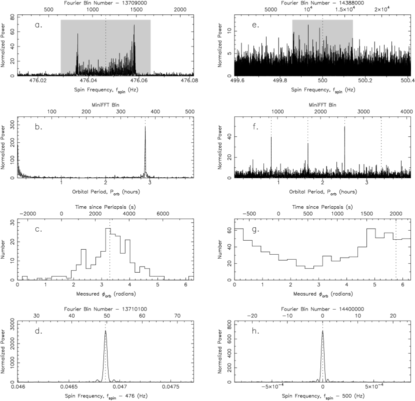
Figure 5: Two examples of key parts of a phase modulation sideband search. The left column shows the analysis of an 8 h observation of the globular cluster 47 Tucanae taken with the Parkes radio telescope of the binary millisecond pulsar 47TucJ. The right column shows analysis of simulated data containing a weaker millisecond pulsar. Plots $a$ and $e$ show portions of the full length power spectra $P(r)$ centered on the fundamental spin harmonics $r_{spin}=f_{spin}T_{obs}$ of the pulsars. The grey regions are the sections of the power spectra $P(r)$ that were Fourier analyzed in order to create the power spectra $P_{2}(r)$ shown in plots $b$ and $f$. Plots $c$ and $g$ show histograms of the orbital phase as measured using the raw Fourier amplitudes in the original FFTs as described in §4.2.2. Once the three Keplerian elements for circular orbits were determined, a Fourier domain orbital template was calculated and correlated with the raw Fourier amplitudes (plots $d$ and $h$). This process recovered all of the power from the pulsar’s fundamental spin harmonic that had initially (plots $a$ and $e$) been spread over many Fourier bins. The dotted lines in each plot show the known values of the independent variable. A more detailed description of each plot is given in §4.2.

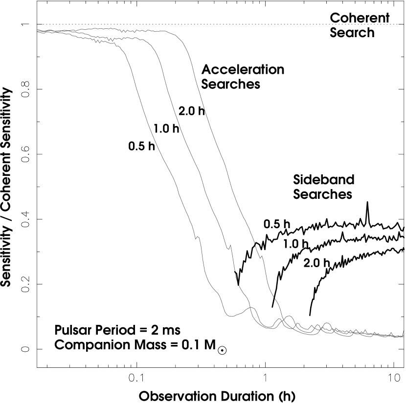
Figure 6: The results of simulations showing the sensitivity of both acceleration and sideband searches for the fundamental harmonic (i.e. a sinusoid) of a 2 ms binary pulsar with a 0.1 $\mbox{M}_{\odot}$ companion and orbital periods of 0.5, 1, and 2 h as a fraction of the optimal (i.e. coherent) sensitivity, which is proportional to $T_{obs}^{-1/2}$. The detection threshold used in the simulations was $8\,\sigma$. Sideband searches are significantly more sensitive to binary pulsars than optimal duration acceleration searches when $T_{obs}\gtrsim 2P_{orb}$.

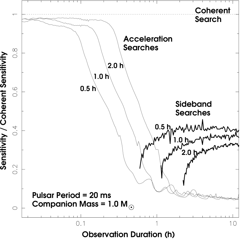
Figure 7: Results from simulations similar to those shown in Figure 6 but for a 20 ms binary pulsar with a $1.0$ $\mbox{M}_{\odot}$ companion.

References

- Anderson (1992) Anderson, S. B. 1992, PhD thesis, California Institute of Technology
- Anderson et al. (1990) Anderson, S. B., Gorham, P. W., Kulkarni, S. R., Prince, T. A., & Wolszczan, A. 1990, Nature, 346, 42
- Arfken (1985) Arfken, G. 1985, Mathematical Methods for Physicists, 3rd edition (San Diego: Academic Press)
- Camilo et al. (2000) Camilo, F., Lorimer, D. R., Freire, P., Lyne, A. G., & Manchester, R. N. 2000, ApJ, 535, 975
- Chou et al. (2001) Chou, Y., Grindlay, J. E., & Bloser, P. F. 2001, ApJ, 549, 1135
- D’Amico et al. (2001) D’Amico, N., Lyne, A. G., Manchester, R. N., Possenti, A., & Camilo, F. 2001, ApJ, 548, L171
- Davies & Hansen (1998) Davies, M. B. & Hansen, B. M. S. 1998, MNRAS, 301, 15
- Galloway et al. (2002) Galloway, D. K., Chakrabarty, D., Morgan, E. H., & Remillard, R. A. 2002, ApJ, 576, L137
- Glendenning (1995) Glendenning, N. K. 1995, ApJ, 440, 881
- Groth (1975) Groth, E. J. 1975, ApJS, 29, 285
- Johnston & Kulkarni (1991) Johnston, H. M. & Kulkarni, S. R. 1991, ApJ, 368, 504
- Jouteux et al. (2002) Jouteux, S., Ramachandran, R., Stappers, B. W., Jonker, P. G., & van der Klis, M. 2002, A&A, 384, 532