The Cosmic Microwave Background & Inflation,
Then & Now

Abstract

The most recent results from the Boomerang, Maxima, DASI, CBI and VSA CMB experiments significantly increase the case for accelerated expansion in the early universe (the inflationary paradigm) and at the current epoch (dark energy dominance). This is especially so when combined with data on high redshift supernovae (SN1) and large scale structure (LSS), encoding information from local cluster abundances, galaxy clustering, and gravitational lensing. There are “7 pillars of Inflation” that can be shown with the CMB probe, and at least 5, and possibly 6, of these have already been demonstrated in the CMB data: (1) the effects of a large scale gravitational potential, demonstrated with COBE/DMR in 1992-96; (2) acoustic peaks/dips in the angular power spectrum of the radiation, which tell about the geometry of the Universe, with the large first peak convincingly shown with Boomerang and Maxima data in 2000, a multiple peak/dip pattern shown in data from Boomerang and DASI (2nd, 3rd peaks, first and 2nd dips in 2001) and from CBI (2nd, 3rd, 4th, 5th peaks, 3rd, 4th dips at 1-sigma in 2002); (3) damping due to shear viscosity and the width of the region over which hydrogen recombination occurred when the universe was 400000 years old (CBI 2002); (4) the primary anisotropies should have a Gaussian distribution (be maximally random) in almost all inflationary models, the best data on this coming from Boomerang; (5) secondary anisotropies associated with nonlinear phenomena subsequent to 400000 years, which must be there and may have been detected by CBI and another experiment, BIMA. Showing the 5 “pillars” involves detailed confrontation of the experimental data with theory; e.g., (5) compares the CBI data with predictions from two of the largest cosmological hydrodynamics simulations ever done. DASI, Boomerang and CBI in 2002, AMiBA in 2003, and many other experiments have the sensitivity to demonstrate the next pillar, (6) polarization, which must be there at the $\sim 7\%$ level. A broad-band DASI detection consistent with inflation models was just reported. A 7th pillar, anisotropies induced by gravity wave quantum noise, could be too small to detect. A minimal inflation parameter set, $\{\omega_{b},\omega_{cdm},\Omega_{tot},\Omega_{Q},w_{Q},n_{s},\tau_{C},\sigma_{8}\}$, is used to illustrate the power of the current data. After marginalizing over the other cosmic and experimental variables, we find the current CMB+LSS+SN1 data give $\Omega_{tot}=1.00^{+.07}_{-.03}$, consistent with (non-baroque) inflation theory. Restricting to $\Omega_{tot}=1$, we find a nearly scale invariant spectrum, $n_{s}=0.97^{+.08}_{-.05}$. The CDM density, $\omega_{cdm}=\Omega_{cdm}{\rm h}^{2}=.12^{+.01}_{-.01}$, and baryon density, $\omega_{b}\equiv\Omega_{b}{\rm h}^{2}=.022^{+.003}_{-.002}$, are in the expected range. (The Big Bang nucleosynthesis estimate is $0.019\pm 0.002$.) Substantial dark (unclustered) energy is inferred, $\Omega_{Q}\approx 0.68\pm 0.05$, and CMB+LSS $\Omega_{Q}$ values are compatible with the independent SN1 estimates. The dark energy equation of state, crudely parameterized by a quintessence-field pressure-to-density ratio $w_{Q}$, is not well determined by CMB+LSS ($w_{Q}<-0.4$ at 95% CL), but when combined with SN1 the resulting $w_{Q}<-0.7$ limit is quite consistent with the $w_{Q}$=$-1$ cosmological constant case.

1 A Synopsis of CMB Experiments

We are in the midst of a remarkable outpouring of results from the CMB that has seen major announcements in each of the last three years, with no sign of abatement in the pace as more experiments are scheduled to release analyses of their results. This paper is an update of capp00 to take into account how the new data have improved the case for primordial acceleration, and for acceleration occurring now. The simplest inflation models are strongly preferred by the data. This does not mean inflation is proved, it just fits the available information better than ever. It also does not mean that competitor theories are ruled out, but they would have to look awfully like inflation for them to work. As a result many competitors have now fallen into extreme disfavour as the data have improved.

The CMB Spectrum: The CMB is a nearly perfect blackbody of $2.725\pm 0.002\,K$ matherTcmb , with a $3.372\pm 0.007\,mK$ dipole associated with the 300 ${\rm~{}km~{}s^{-1}}$ flow of the earth in the CMB, and a rich pattern of higher multipole anisotropies at tens of $\mu$K arising from fluctuations at photon decoupling and later. Spectral distortions from the blackbody have been detected in the COBE FIRAS and DIRBE data. These are associated with starbursting galaxies due to stellar and accretion disk radiation downshifted into the infrared by dust then redshifted into the submillimetre; they have energy about twice all that in optical light, about a tenth of a percent of that in the CMB. The spectrally well-defined Sunyaev-Zeldovich (SZ) distortion associated with Compton-upscattering of CMB photons from hot gas has not been observed in the spectrum. The FIRAS 95% CL upper limit of $6.0\times 10^{-5}$ of the energy in the CMB is compatible with the $\mathrel{\hbox to0.0pt{\lower 3.0pt\hbox{$\mathchar 536\relax$}\hss}\raise 2.0pt\hbox{$\mathchar 316\relax$}}10^{-5}$ expected from clusters, groups and filaments in structure formation models, and places strong constraints on the allowed amount of earlier energy injection, e.g., ruling out mostly hydrodynamic models of LSS. The SZ effect has been well observed at high resolution with very high signal-to-noise along lines-of-sight through dozens of clusters. The SZ effect in random fields may have been observed with the CBI and BIMA, again at high resolution, although multifrequency observations to differentiate the signal from the CMB primary and radio source contributions will be needed to show this.

The Era of Upper Limits: The story of the experimental quest for spatial anisotropies in the CMB temperature is a heroic one. The original 1965 Penzias and Wilson discovery paper quoted angular anisotropies below $10\%$, but by the late sixties $10^{-3}$ limits were reached, by Partridge and Wilkinson and by Conklin and Bracewell. As calculations of baryon-dominated adiabatic and isocurvature models improved in the 70s and early 80s, the theoretical expectation was that the experimentalists just had to get to $10^{-4}$, as they did, e.g., Boynton and Partridge in 73. The only signal found was the dipole, hinted at by Conklin and Bracewell in 73, but found definitively in Berkeley and Princeton balloon experiments in the late 70s, along with upper limits on the quadrupole. Throughout the 1980s, the upper limits kept coming down, punctuated by a few experiments widely used by theorists to constrain models: the small angle 84 Uson and Wilkinson and 87 OVRO limits, the large angle 81 Melchiorri limit, early (87) limits from the large angle Tenerife experiment, the small angle RATAN-600 limits, the $7^{\circ}$-beam Relict-1 satellite limit of 87, and Lubin and Meinhold’s 89 half-degree South Pole limit, marking a first assault on the peak.

Primordial fluctuations from which structure would have grown in the Universe can be one of two modes: adiabatic scalar perturbations associated with gravitational curvature variations or isocurvature scalar perturbations, with no initial curvature variation, but variations in the relative amounts of matter of different types, e.g., in the number of photons per baryon, or per dark matter particle, i.e., in the entropy per particle. Both modes could be present at once, and in addition there may also be tensor perturbations associated with primordial gravitational radiation which can leave an imprint on the CMB. The statistical distribution of the primordial fluctuations determines the statistics of the radiation pattern; e.g., the distribution could be generically non-Gaussian, needing an infinity of N-point correlation functions to characterize it. The special case when only the 3D 2-point correlation function is needed is that of a Gaussian random field; if dependent upon spatial separations only, not absolute positions or orientations, it is homogeneous and isotropic. The radiation pattern is then a 2D Gaussian field fully specified by its correlation function, whose spherical transform is the angular power spectrum, ${\cal C}_{\ell}$, where $\ell$ is the multipole number. If the 3D correlation does not depend upon multiplication by a scale factor, it is scale invariant. This does not translate into scale invariance in the 2D radiation correlation, whose features reflect the physical transport processes of the radiation through photon decoupling.

The upper limit experiments were in fact highly useful in ruling out broad ranges of theoretical possibilities. In particular adiabatic baryon-dominated models were ruled out. In the early 80s, universes dominated by dark matter relics of the hot Big Bang lowered theoretical predictions by about an order of magnitude over those of the baryon-only models. In the 82 to mid-90s period, many groups developed codes to solve the perturbed Boltzmann–Einstein equations when such collisionless relic dark matter was present. Armed with these pre-COBE computations, plus the LSS information of the time, a number of otherwise interesting models fell victim to the data: scale invariant isocurvature cold dark matter models in 86, large regions of parameter space for isocurvature baryon models in 87, inflation models with radically broken scale invariance leading to enhanced power on large scales in 87-89, CDM models with a decaying ($\sim{\rm keV}$) neutrino if its lifetime was too long ($\mathrel{\hbox to0.0pt{\lower 3.0pt\hbox{$\mathchar 536\relax$}\hss}\raise 2.0pt\hbox{$\mathchar 318\relax$}}10{\rm yr}$) in 87 and 91. Also in this period there were some limited constraints on ”standard” CDM models, restricting $\Omega_{tot}$, $\Omega_{B}$, and the amplitude parameter $\sigma_{8}$. ($\sigma_{8}^{2}$ is a bandpower for density fluctuations on a scale associated with rare clusters of galaxies, $8{\,{\rm h}^{-1}~{}\rm Mpc}$, where ${\rm h}=H_{0}/(100{\rm~{}km~{}s^{-1}}{\rm~{}Mpc}^{-1})$.)

DMR and Post-DMR Experiments to April 1999: The familiar motley pattern of anisotropies associated with $2\mathrel{\hbox to0.0pt{\lower 3.0pt\hbox{$-$}\hss}\raise 2.0pt\hbox{$\mathchar 316\relax$}}\ell\mathrel{\hbox to0.0pt{\lower 3.0pt\hbox{$\mathchar 536\relax$}\hss}\raise 2.0pt\hbox{$\mathchar 316\relax$}}20$ multipoles at the $30\mu K$ level revealed by COBE at $7^{\circ}$ resolution was shortly followed by detections, and a few upper limits (UL), at higher $\ell$ in 19 other ground-based (gb) or balloon-borne (bb) experiments — most with many fewer resolution elements than the 600 or so for COBE. Some predated in design and even in data delivery the 1992 COBE announcement. We have the intermediate angle SP91 (gb), the large angle FIRS (bb), both with strong hints of detection before COBE, then, post-COBE, more Tenerife (gb), MAX (bb), MSAM (bb), white-dish (gb, UL), argo (bb), SP94 (gb), SK93-95 (gb), Python (gb), BAM (bb), CAT (gb), OVRO-22 (gb), SuZIE (gb, UL), QMAP (bb), VIPER (gb) and Python V (gb). A list valid to April 1999 with associated bandpowers is given in BJK2000 , and are referred here as 4.99 data. They showed evidence for a first peak BJK2000 , although it was not well localized. A strong first peak, followed by a sequence of smaller peaks diminished by damping in the ${\cal C}_{\ell}$ spectrum was a long-standing prediction of adiabatic models. For restricted parameter sets, good constraints were given on $n_{s}$, and on $\Omega_{tot}$ and $\Omega_{\Lambda}$ when LSS was added bj99 .

TOCO, BOOMERANG & MAXIMA: The picture dramatically improved over the 3 years since April 1999. In summer 99, the ground-based TOCO experiment in Chile toco98 , and in November 99 the North American balloon test flight of Boomerang mauskopf99 , gave results that greatly improved first-peak localization, pointing to $\Omega_{tot}\sim 1$. Then in April 2000 dramatic results from the first CMB long duration balloon (LDB) flight, Boomerang debernardis00 ; lange00 , were announced, followed in May 2000 by results from the night flight of Maxima Maxima00 . Boomerang’s best resolution was $10.7^{\prime}\pm 1.4^{\prime}$, about 40 times better than that of COBE, with tens of thousands of resolution elements. (The corresponding Gaussian beam filtering scale in multipole space is $\ell_{s}\sim 800$.) Maxima had a similar resolution but covered an order of magnitude less sky. In April 2001, the Boomerang analysis was improved and much more of the data were included, delivering information on the spectrum up to $\ell\sim 1000$ Netterfield01 ; deBernardis01 . Maxima also increased its $\ell$ range Maxima01 .

Boomerang carried a 1.2m telescope with 16 bolometers cooled to 300 mK in the focal plane aloft from McMurdo Bay in Antarctica in late December 1998, circled the Pole for 10.6 days and landed just 50 km from the launch site, only slightly damaged. Maps at 90, 150 and 220 GHz showed the same basic spatial features and the intensities were shown to fall precisely on the CMB blackbody curve. The fourth frequency channel at 400 GHz is dust-dominated. Fig. 1 shows a 150 GHz map derived using four of the six bolometers at 150 GHz. There were 10 bolometers at the other frequencies. Although Boomerang altogether probed 1800 square degrees, the April 2000 analysis used only one channel and 440 sq. deg., and the April 2001 analyses used 4 channels and the region in the ellipse covering 800 sq. deg. That is the Boomerang data used in this paper. In Ruhl02 , the coverage is extended to 1200 sq deg, 2.9% of the sky.

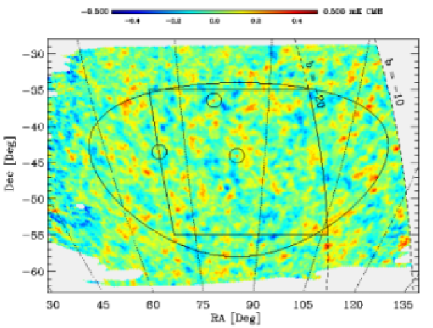
Figure 1: The Boomerang 150 GHz bolometer map is shown in the top figure. Of the entire 1800 square degrees covered, only the interior 800 sq. degs. (within the ellipse) were used in Netterfield01 and this analysis. In the April 2000 analysis only one channel within the rectangle was used. In the Ruhl et al., 2002 analysis, essentially the entire region is covered. The three circles show regions cut out of the analysis because they contain quasars with emission at 150 GHz. The resolution is $10.7^{\prime}\pm 1.4^{\prime}$ fwhm.

Maxima covered a 124 square degree region of sky in the Northern Hemisphere. Though Maxima was not an LDB, it did well because its bolometers were cooled even more than Boomerang’s, to 100 mK, leading to higher sensitivity per unit observing time, it had a star camera so the pointing was well determined, and, further, all frequency channels were used in its analysis.

DASI, CBI & VSA: DASI (the Degree Angular Scale Interferometer), located at the South Pole, has 13 dishes of size 0.2m. Instead of bolometers, it uses HEMTs, operating at 10 frequency channels spanning the band $26-36$GHz. An interferometer baseline directly translates into a Fourier mode on the sky. The dish spacing and operating frequency dictate the $\ell$ range. In DASI’s case, the range covered is $125\mathrel{\hbox to0.0pt{\lower 3.0pt\hbox{$\mathchar 536\relax$}\hss}\raise 2.0pt\hbox{$\mathchar 316\relax$}}\ell\mathrel{\hbox to0.0pt{\lower 3.0pt\hbox{$\mathchar 536\relax$}\hss}\raise 2.0pt\hbox{$\mathchar 316\relax$}}900$. 32 independent maps were constructed, each of size $3.4^{\circ}$, the field-of-view (fov). The total area covered was 288 sq. deg. DASI’s spectacular results were also announced in April 2001, unveiling a spectrum close to that reported by Boomerang at the same time. The two results together reinforced each other and lent considerable confidence to the emerging ${\cal C}_{\ell}$ spectrum in the $\ell<1000$ regime.

CBI (the Cosmic Background Imager), based at 16000 feet on a high plateau in Chile, is the sister experiment to DASI. It has 13 0.9m dishes operating in the same HEMT channels as DASI. The instrument measures 78 baselines simultaneously. The larger dishes by a factor of 4 and longer baselines imply higher resolution by about the same factor: the CBI results reported in May 2002 go to $\ell$ of 3500, a huge increase over Boomerang, Maxima and DASI. Only the analyses of data from the year 2000 observing campaign were reported. During 2000, CBI covered three deep fields of diameter roughly $0.75^{\circ}$ Mason02b , and three mosaic regions, each of size roughly 13 square degrees Pearson02 . In analyzing such high resolution data at 30 GHz, great attention must be paid to the contamination by point sources, but we are confident that this is handled well Mason02b . Data from 2001 roughly doubles the amount, increases the area covered, and its analysis is currently underway.

Fig. 2 shows one of the CBI mosaic regions of the sky and Fig. 3 one of the deep regions.

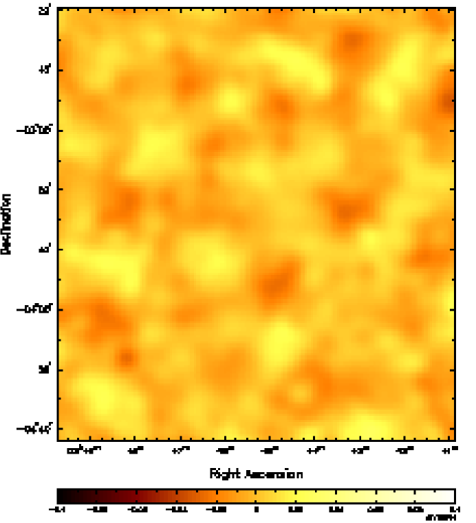
Figure 2: The inner 2.5 degrees of one of the three 13 square degree CBI mosaic fields is shown. The mosaic image is a standard radio astronomy map, with point sources removed. The regions are smaller than Boomerang covered, but the resolution is a factor of at least three better. The mass subtended by the CBI resolution scale ($\sim 4^{\prime}$) easily encompasses the mass that collapses later in the universe to generate clusters of galaxies.

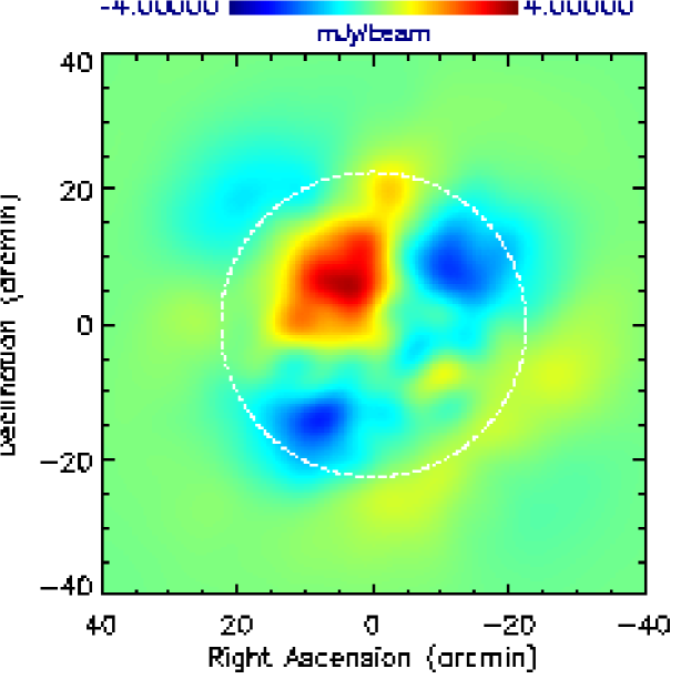
Figure 3: An 0.75 degree field-of-view (within the circle) Wiener-filtered map of one of the three deep CBI fields is shown. Apart from the primary anisotropy signal, the deep images contain power at high $\ell$ that might be from the SZ effect in collapsed clusters at redshift of order 1. We know that the predicted SZ signal is near to that seen, and is very sensitive to $\sigma_{8}$ (${\cal C}_{\ell}^{(SZ)}\propto\sigma_{8}^{7}$). $\sigma_{8}\approx 1$ is needed for the SZ effect as determined by hydro simulations to agree with the data. The primary CMB data prefer values between 0.8 and 0.9, and so although we do expect the SZ signal to be lurking within the CBI signal, it may not be quite as large as the extra power seen in these deep maps.

The VSA (Very Small Array) in Tenerife, also an interferometer, operating at 30 GHz, covered the $\ell$ range of DASI, and confirmed the spectrum emerging from the Boomerang, Maxima and DASI data in that region. The VSA is now observing at longer baselines to increase its $\ell$ range.

The Optimal Spectrum, circa Summer 2002: The power spectrum shown in Fig. 4 combines all of the data in a way that takes all of the uncertainties in each experiment (calibration and beam) into account. The point at small $\ell$ is dominated by DMR, at $900\mathrel{\hbox to0.0pt{\lower 3.0pt\hbox{$\mathchar 536\relax$}\hss}\raise 2.0pt\hbox{$\mathchar 316\relax$}}\ell\mathrel{\hbox to0.0pt{\lower 3.0pt\hbox{$\mathchar 536\relax$}\hss}\raise 2.0pt\hbox{$\mathchar 316\relax$}}2000$ by the CBI mosaic data, with that beyond 2000 by the CBI deep data. In between, Boomerang drives the small error bars, DASI and CBI set the calibration and beam of Boomerang and give spectra totally compatible with Boomerang. Both VSA and Maxima are in agreement with this data as well. Further, although the errors from the experiments before April 2000 are larger, the quite heterogeneous 4.99+TOCO+Boomerang-NA mix of CMB data is very consistent with what the newer experiments show. It is an amazing concordance of data. Accompanying this story is a convergence with decreasing errors over time on the values of the cosmological parameters given in Table 1.

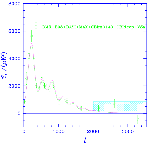
Figure 4: The ${\cal C}_{\ell}$ are defined in terms of CMB temperature anisotropy multipoles by ${\cal C}_{\ell}\equiv\ell(\ell+1){\langle|(\Delta T/T)_{\ell m}|^{2}\rangle}/(2\pi)$. The optimal ${\cal C}_{\ell}$ spectrum corresponds to a maximum-likelihood fit to the power in bands marginalized over beam and calibration uncertainties of the various experiments, This one uses “all-data” (DMR + Boomerang + Maxima + DASI + CBI mosaic + CBI deep + VSA + TOCO + Boomerang-NA + the 4.99 data). A $\Delta\ell=75$ binning was chosen up to $\sim 800$, going over to the CBI deep binning at large $\ell$. The $\ell>2000$ excess found with the deep CBI data is denoted by the light blue hatched region (95% confidence limit). Two best fit models to “all-data” are shown. They are both $\Lambda$CDM models; e.g., the upper curve (magenta) has parameters $\{\Omega_{\rm{tot}}$, $\Omega_{\Lambda}$, $\Omega_{b}h^{2}$, $\Omega_{\rm cdm}h^{2}$, $n_{s}$, $\tau_{C}\}$=$\{1.0,0.7,0.02,0.14,0.975,0\}$.

Primary CMB Processes and Soundwave Maps at Decoupling: Boomerang, Maxima, DASI, CBI and VSA were designed to measure the primary anisotropies of the CMB, those which can be calculated using linear perturbation theory. What we see in Figs. 1, 2 are, basically, images of soundwave patterns that existed about 400,000 years after the Big Bang, when the photons were freed from the plasma. The visually evident structure on degree scales is even more apparent in the power spectra of the maps, which show a dominant (first acoustic) peak, with less prominent subsequent ones detected at varying levels of statistical significance.

The images are actually a projected mixture of dominant and subdominant physical processes through the photon decoupling ”surface”, a fuzzy wall at redshift $z_{dec}\approx 1050$, when the Universe passed from optically thick to thin to Thomson scattering over a comoving distance $\approx 19{\rm~{}Mpc}$. Prior to this, acoustic wave patterns in the tightly-coupled photon-baryon fluid on scales below the comoving ”sound crossing distance” at decoupling, $\mathrel{\hbox to0.0pt{\lower 3.0pt\hbox{$\mathchar 536\relax$}\hss}\raise 2.0pt\hbox{$\mathchar 316\relax$}}150{\rm~{}Mpc}$ (i.e., $\mathrel{\hbox to0.0pt{\lower 3.0pt\hbox{$\mathchar 536\relax$}\hss}\raise 2.0pt\hbox{$\mathchar 316\relax$}}150{\rm~{}kpc}$ physical), were viscously damped, strongly so on scales below the $\approx 10{\rm~{}Mpc}$ damping scale. After, photons freely-streamed along geodesics to us, mapping (through the angular diameter distance relation) the post-decoupling spatial structures in the temperature to the angular patterns we observe now as the primary anisotropies. The maps are images projected through the fuzzy decoupling surface of the acoustic waves (photon bunching), the electron flow (Doppler effect) and the gravitational potential peaks and troughs (”naive” Sachs-Wolfe effect) back then. Free-streaming along our (linearly perturbed) past light cone leaves the pattern largely unaffected, except that temporal evolution in the gravitational potential wells as the photons propagate through them leaves a further $\Delta T$ imprint, called the integrated Sachs-Wolfe effect. Intense theoretical work over three decades has put accurate calculations of this linear cosmological radiative transfer on a firm footing, and there are speedy, publicly available and widely used codes for evaluation of anisotropies in a variety of cosmological scenarios, “CMBfast” and “CAMB” cmbfast . Extensions to more cosmological models have been added by a variety of researchers.

Of course there are a number of nonlinear effects that are also present in the maps. These secondary anisotropies include weak-lensing by intervening mass, Thomson-scattering by the nonlinear flowing gas once it became ”reionized” at $z\sim 10$, the thermal and kinematic SZ effects, and the red-shifted emission from dusty galaxies. They all leave non-Gaussian imprints on the CMB sky.

The Immediate Future: Results are in and the analysis is underway for the bolometer single dish ACBAR experiment based at the South Pole (with about $5^{\prime}$ resolution, allowing coverage to $\ell\sim 2000$). Results from two balloon flights, Archeops and Tophat, are also expected soon. MINT, a Princeton interferometer, also has results soon to be released.

In June 2001, NASA launched the all-sky HEMT-based MAP satellite, with $12^{\prime}$ resolution. We expect spectacularly accurate results covering the $\ell$ range to about 600 to be announced in Jan. 2003, with higher $\ell$ and smaller errors expected as the observing period increases. Eventually four years of data are expected.

Further downstream, in 2007, ESA will launch the bolometer+HEMT-based Planck satellite, with $5^{\prime}$ resolution.

Targeting Polarization of the Primary CMB Signal: The polarization dependence of Compton scattering induces a well defined polarization signal emerging from photon decoupling. Given the total ${\cal C}_{\ell}$ of Fig. 4, we can forecast what the strength of that signal and its cross-correlation with the total anisotropy will be, and which $\ell$ range gives the maximum signal: $\sim 5\mu$K over $\ell\sim 400-1600$ is a target for the “$E$-mode” that scalar fluctuations give.

A great race was on to first detect the $E$-mode. Experiments range from many degrees to subarcminute scales. DASI has analyzed 271 days of polarization data on 2 deep fields ($3.4^{\circ}$ fov) and just announced a $5\sigma$ detection at a level consistent with inflation-based models DASIpol02 . Boomerang will fly again, in December 2002, with polarization-sensitive bolometers of the kind that will also be used on Planck; as well, MAXIMA will fly again as the polarization-targeting MAXIPOL; the detectors on CBI have been reconfigured to target polarization and the CBI is beginning to take data; MAP can also measure polarization with its HEMTs. Other experiments, operating or planned include AMiBA, COMPASS, CUPMAP, PIQUE and its sequel, POLAR, Polarbear, Polatron, QUEST, Sport/BaRSport, BICEP, among others. The amplitude of the DASI E detection is $0.8\pm 0.3$ of the forecasted amplitude from the total anisotropy data; the cross-correlation of the polarization with the total anisotropy has also been detected, with amplitude $0.9\pm 0.4$ of the forecast. These detections used a broad-band shape covering the $\ell$ range $\sim 250-750$ derived from the theoretical forecasts. The forecasts indicate solid detections with enough well-determined bandpowers for use in cosmological parameter studies are soon likely.

We cannot yet forecast the strength of the “$B$-mode” signal induced by gravity waves, since there is as yet no evidence for or against them in the data. However, the amplitude would be very small indeed even at $\ell\sim 100$. Nonetheless there are experiments such as BICEP (Caltech) being planned to go after polarization in these low $\ell$ ranges.

Targeting Secondary Anisotropies: SZ anisotropies have been probed by single dishes, the OVRO and BIMA mm arrays, and the Ryle interferometer. Detections of individual clusters are now routine. The power at $\ell>2000$ seen in the CBI deep data (Fig. 4) Mason02b and in the BIMA data at $\ell\sim 6000$ BIMA02 may be due to the SZ effect in ambient fields, e.g., Bond02 . A number of planned HEMT-based interferometers are being built with this ambient effect as a target: CARMA (OVRO+BIMA together), the SZA (Chicago, to be incorporated in CARMA), AMI (Britain, including the Ryle telescope), and AMiBA (Taiwan). Bolometer-based experiments will also be used to probe the SZ effect, including the CSO (Caltech submm observatory, a 10m dish) with BOLOCAM on Mauna Kea, ACBAR at the South Pole and the LMT (large mm telescope, with a 50 metre dish) in Mexico. As well, APEX, a 12 m German single dish, Kobyama, a 10 m Japanese single dish, and the 100m Green Bank telescope can all be brought to bear down on the SZ sky. Very large bolometer arrays with thousands of elements are planned: the South Pole Telescope (SPT, Chicago) and the Atacama Cosmology Telescope (ACT, Princeton), with resolution below $2^{\prime}$, will be powerful probes of the SZ effect as well as of primary anisotropies.

Anisotropies from dust emission from high redshift galaxies are being targeted by the JCMT with the SCUBA bolometer array, the OVRO mm interferometer, the CSO, the SMA (submm array) on Mauna Kea, the LMT, the ambitious US/ESO ALMA mm array in Chile, the LDB BLAST, and ESA’s Herschel satellite. About $50\%$ of the submm background has so far been identified with sources that SCUBA has found.

The CMB Analysis Pipeline: Analyzing Boomerang and other single-dish experiments involves a pipeline, reviewed in bc01 , that takes the timestream in each of the bolometer channels coming from the balloon plus information on where it is pointing and turns it into spatial maps for each frequency characterized by average temperature fluctuation values in each pixel (Fig. 1) and a pixel-pixel correlation matrix characterizing the noise. From this, various statistical quantities are derived, in particular the temperature power spectrum as a function of multipole, grouped into bands, and band-band error matrices which together determine the full likelihood distribution of the bandpowers BJK98 ; BJK2000 . Fundamental to the first step is the extraction of the sky signal from the noise, using the only information we have, the pointing matrix mapping a bit in time onto a pixel position on the sky. In the April 2001 analysis of Boomerang, and subsequent work, powerful use of Monte Carlo simulations was made to evaluate the power spectrum and other statistical indicators in maps with many more pixels than was possible with conventional matrix methods for estimating power spectra Netterfield01 .

For interferometer experiments, the basic data are visibilities as a function of baseline and frequency, with contributions from random detector noise as well as from the sky signals. As mentioned above, a baseline is a direct probe of a given angular wavenumber vector on the sky, hence suggests we should make “generalized maps” in “momentum space” (i.e., Fourier transform space) rather than in position space, as for Boomerang. A major advance was made in Myers02 to deal with the large volume of interferometer data that we got with CBI, especially for the mosaics with their large number of overlapping fields. We “optimally” compressed the $>{\cal O}(10^{5})$ visibility measurements of each field into a $<{\cal O}(10^{4})$ coarse grained lattice in momentum space, and used the information in that “generalized pixel” basis to estimate the power spectrum and statistical distribution of the signals.

There is generally another step in between the maps and the final power spectra, namely separating the multifrequency spatial maps into the physical components on the sky: the primary CMB, the thermal and kinematic Sunyaev-Zeldovich effects, the dust, synchrotron and bremsstrahlung Galactic signals, the extragalactic radio and submillimetre sources. The strong agreement among the Boomerang maps indicates that to first order we can ignore this step, but it has to be taken into account as the precision increases.

Because of the 1 cm observing wavelength of CBI and its resolution, the contribution from extragalactic radio sources is significant. We project out of the data sets known point sources when estimating the primary anisotropy spectrum by using a number of constraint matrices. The positions are obtained from the (1.4 GHz) NVSS catalog. When projecting out the sources we use large amplitudes which effectively marginalize over all affected modes. This insures robustness with respect to errors in the assumed fluxes of the sources. The residual contribution of sources below our known-source cutoff is treated as a white noise background with an amplitude (and error) estimated as well from the NVSS database Mason02b .

The CMB Statistical Distributions are Nearly Gaussian: The primary CMB fluctuations are quite Gaussian, according to COBE, Maxima, and now Boomerang and CBI analyses. Analysis of data like that in the Fig. 1 map show a one-point distribution of temperature anisotropy values that is well fit by a Gaussian distribution. Higher order (concentration) statistics (3,4-point functions, etc.) tell us of non-Gaussian aspects, necessarily expected from the Galactic foreground and extragalactic source signals, but possible even in the early Universe fluctuations. For example, though non-Gaussianity occurs only in the more baroque inflation models of quantum noise, it is a necessary outcome of defect-driven models of structure formation. (Peaks compatible with Fig. 4 do not appear in non-baroque defect models, which now appear highly unlikely.) There is currently no evidence for a breakdown of the Gaussianity in the 150 GHz maps as long as one does not include regions near the Galactic plane in the analysis. We have also found that the one-point distribution of the CBI data is also compatible with a Gaussian. However, since we know non-Gaussianity is necessarily there at some level, more exploration is needed.

Though great strides have been made in the analysis of the Boomerang-style and CBI-style experiments, there is intense effort worldwide developing fast and accurate algorithms to deal with the looming megapixel datasets of LDBs and the satellites. Dealing more effectively with the various component signals and the statistical distribution of the errors resulting from the component separation is a high priority.

2 Cosmic Parameter Estimation

Parameters of Structure Formation: Following capp00 , we adopt a restricted set of 8 cosmological parameters, augmenting the basic 7 used in lange00 ; jaffe00 ; Netterfield01 ; Sievers02 , $\{\Omega_{\Lambda},\Omega_{k},\omega_{b},\omega_{cdm},n_{s},\tau_{C},\sigma_{8}\}$, by one. The vacuum or dark energy encoded in the cosmological constant $\Omega_{\Lambda}$ is reinterpreted as $\Omega_{Q}$, the energy in a scalar field $Q$ which dominates at late times, which, unlike $\Lambda$, could have complex dynamics associated with it. $Q$ is now often termed a quintessence field. One popular phenomenology is to add one more parameter, $w_{Q}=p_{Q}/\rho_{Q}$, where $p_{Q}$ and $\rho_{Q}$ are the pressure and density of the $Q$-field, related to its kinetic and potential energy by $\rho_{Q}=\dot{Q}^{2}/2+(\nabla Q)^{2}/2+V(Q)$, $p_{Q}=\dot{Q}^{2}/2-(\nabla Q)^{2}/6-V(Q)$. Thus $w_{Q}=-1$ for the cosmological constant. Spatial fluctuations of $Q$ are expected to leave a direct imprint on the CMB for small $\ell$. This will depend in detail upon the specific model for $Q$. We ignore this complication here, but caution that using DMR data which is sensitive to low $\ell$ behaviour in conjunction with the rest will give somewhat misleading results. To be self consistent, a model must be complete: e.g., even the ludicrous models with constant $w_{Q}$ would have necessary fluctuations to take into account. As well, as long as $w_{Q}$ is not exactly $-1$, it will vary with time, but the data will have to improve for there to be sensitivity to this, and for now we can just interpret $w_{Q}$ as an appropriate time-average of the equation of state. The curvature energy $\Omega_{k}\equiv 1-\Omega_{tot}$ also can dominate at late times, as well as affecting the geometry.

We use only 2 parameters to characterize the early universe primordial power spectrum of gravitational potential fluctuations $\Phi$, one giving the overall power spectrum amplitude ${\cal P}_{\Phi}(k_{n})$, and one defining the shape, a spectral tilt $n_{s}(k_{n})\equiv 1+d\ln{\cal P}_{\Phi}/d\ln k$, at some (comoving) normalization wavenumber $k_{n}$. We really need another 2, ${\cal P}_{GW}(k_{n})$ and $n_{t}(k_{n})$, associated with the gravitational wave component. In inflation, the amplitude ratio is related to $n_{t}$ to lowest order, with ${\cal O}(n_{s}-n_{t})$ corrections at higher order, e.g., bh95 . There are also useful limiting cases for the $n_{s}-n_{t}$ relation. However, as one allows the baroqueness of the inflation models to increase, one can entertain essentially any power spectrum (fully $k$-dependent $n_{s}(k)$ and $n_{t}(k)$) if one is artful enough in designing inflaton potential surfaces. Actually $n_{t}(k)$ does not have as much freedom as $n_{s}(k)$ in inflation. For example, it is very difficult to get $n_{t}(k)$ to be positive. As well, one can have more types of modes present, e.g., scalar isocurvature modes (${\cal P}_{is}(k_{n}),n_{is}(k)$) in addition to, or in place of, the scalar curvature modes (${\cal P}_{\Phi}(k_{n}),n_{s}(k)$). However, our philosophy is consider minimal models first, then see how progressive relaxation of the constraints on the inflation models, at the expense of increasing baroqueness, causes the parameter errors to open up. For example, with COBE-DMR and Boomerang, we can probe the GW contribution, but the data are not powerful enough to determine much. Planck can in principle probe the gravity wave contribution reasonably well.

We use another 2 parameters to characterize the transport of the radiation through the era of photon decoupling, which is sensitive to the physical density of the various species of particles present then, $\omega_{j}\equiv\Omega_{j}{\rm h}^{2}$. We really need 4: $\omega_{b}$ for the baryons, $\omega_{cdm}$ for the cold dark matter, $\omega_{hdm}$ for the hot dark matter (massive but light neutrinos), and $\omega_{er}$ for the relativistic particles present at that time (photons, very light neutrinos, and possibly weakly interacting products of late time particle decays). For simplicity, though, we restrict ourselves to the conventional 3 species of relativistic neutrinos plus photons, with $\omega_{er}$ therefore fixed by the CMB temperature and the relationship between the neutrino and photon temperatures determined by the extra photon entropy accompanying $e^{+}e^{-}$ annihilation. Of particular importance for the pattern of the radiation is the (comoving) distance sound can have influenced by recombination (at redshift $z_{dec}=a_{dec}^{-1}-1$),

$$r_{s}=6000/\sqrt{3}{\rm~{}Mpc}\int_{0}^{\sqrt{a_{dec}}}(\omega_{m}+\omega_{er}a^{-1})^{-1/2}(1+\omega_{b}a/(4\omega_{\gamma}/3))^{-1/2}\ d\sqrt{a},$$ (1)

where $\omega_{\gamma}=2.46\times 10^{-5}$ is the photon density, $\omega_{er}=1.68\omega_{\gamma}$ for 3 species of massless neutrinos and $\omega_{m}\equiv\omega_{hdm}+\omega_{cdm}+\omega_{b}$.

The angular diameter distance relation maps spatial structure at photon decoupling perpendicular to the line-of-sight with transverse wavenumber $k_{\perp}$ to angular structure, through $\ell={\cal R}_{dec}k_{\perp}$. In terms of the comoving distance to photon decoupling (recombination), $\chi_{dec}$, and the curvature scale $d_{k}$, ${\cal R}_{dec}$ is given by

$${\cal R}_{dec}=\{d_{k}{\rm sinh}(\chi_{dec}/d_{k}),\chi_{dec},d_{k}{\rm sin}(\chi_{dec}/d_{k})\},\ {\rm where}\ d_{k}=3000|\omega_{k}|^{-1/2}{\rm~{}Mpc},$$

$${\rm and}\ \chi_{dec}=6000{\rm~{}Mpc}\int_{\sqrt{a_{dec}}}^{1}(\omega_{m}+\omega_{Q}a^{-6w_{Q}}+\omega_{k}a)^{-1/2}\ d\sqrt{a}\,.$$ (2)

The 3 cases are for negative, zero and positive mean curvature. Thus the mapping depends upon $\omega_{k}$, $\omega_{Q}$ and $w_{Q}$ as well as on $\omega_{m}$. The location of the acoustic peaks $\ell_{pk,j}$ is proportional to the ratio of ${\cal R}_{dec}$ to $r_{s}$, hence depends upon $\omega_{b}$ through the sound speed as well. Thus $\ell_{pk,j}$ defines a functional relationship among these parameters, a degeneracy degeneracies that would be exact except for the integrated Sachs-Wolfe effect, associated with the change of $\Phi$ with time if $\Omega_{Q}$ or $\Omega_{k}$ is nonzero. (If $\dot{\Phi}$ vanishes, the energy of photons coming into potential wells is the same as that coming out, and there is no net impact of the rippled light cone upon the observed $\Delta T$.)

Our 7th parameter is an astrophysical one, the Compton ”optical depth” $\tau_{C}$ from a reionization redshift $z_{reh}$ to the present. It lowers ${\cal C}_{\ell}$ by $\exp(-2\tau_{C})$ at $\ell$’s in the Boomerang/CBI regime. For typical models of hierarchical structure formation, we expect $\tau_{C}\mathrel{\hbox to0.0pt{\lower 3.0pt\hbox{$\mathchar 536\relax$}\hss}\raise 2.0pt\hbox{$\mathchar 316\relax$}}0.2$. It is partly degenerate with $\sigma_{8}$ and cannot quite be determined at this precision by CMB data now.

The LSS also depends upon our parameter set: an important combination is the wavenumber of the horizon when the energy density in relativistic particles equals the energy density in nonrelativistic particles: $k_{Heq}^{-1}\approx 5\Gamma^{-1}{\,{\rm h}^{-1}~{}\rm Mpc}$, where $\Gamma\approx\Omega_{m}{\rm h}\Omega_{er}^{-1/2}$. Instead of ${\cal P}_{\Phi}(k_{n})$ for the amplitude parameter, we often use ${\cal C}_{10}$ at $\ell=10$ for CMB only, and $\sigma_{8}^{2}$ when LSS is added. When LSS is considered in this paper, it refers to constraints on $\Gamma+(n_{s}-1)/2$ and $\ln\sigma_{8}^{2}$ that are obtained by comparison with the data on galaxy clustering, cluster abundances and from weak lensing  Bond02 ; lange00 ; bj99 . At the current time, the constraints from $\sigma_{8}$ from lensing and cluster abundances are stronger thoes from $\Gamma$, although, with the wealth of data emerging from the Sloan Digital Sky Survey and the 2dF redshift survey, shape should soon deliver more powerful information than overall amplitude. However, in the future, weak lensing will allow amplitude and shape to be simultaneously constrained without the uncertainties associated with the biasing of the galaxy distribution wrt the mass that the redshift surveys must deal with.

When we allow for freedom in $\omega_{er}$, the abundance of primordial helium, tilts of tilts ($dn_{\{s,is,t\}}(k_{n})/d\ln k,...$) for 3 types of perturbations, the parameter count would be 17, and many more if we open up full theoretical freedom in spectral shapes. However, as we shall see, as of now only 4 combinations can be determined with 10% accuracy with the CMB. Thus choosing 8 is adequate for the present; 7 of these are discretely sampleddatabase , with generous boundaries, though for drawing cosmological conclusions we adopt a weak prior probability on the Hubble parameter and age: we restrict ${\rm h}$ to lie in the 0.45 to 0.9 range, and the age to be above 10 Gyr.

Peaks, Dips and $\Omega_{tot}$, $\Omega_{Q}$ and $w_{Q}$: For given $\omega_{m}$ and $\omega_{b}$, we show the lines of constant $\ell_{pk,j}\propto{\cal R}_{dec}/r_{s}$ in the $\Omega_{k}$–$\Omega_{Q}$ plane for $w_{Q}$=$-1$ in Fig. 5, and in the $w_{Q}$–$\Omega_{Q}$ plane for $\Omega_{tot}$=1 in Fig. 7, using the formulas given above and in degeneracies .

Our current best estimate Sievers02 of the peak locations $\ell_{pk,j}$, using all current CMB data and the flat+wk-$h$+LSS prior, are $222\pm 3$, $537\pm 6$, $823\pm 45$, $1138\pm 45$, $1437\pm 59$, obtained by forming $\exp<\ln\ell_{pk,j}>$, where the average and variance of $\ln\ell_{pk,j}$ are determined by integrating over the probability-weighted database described above. The interleaving dips are at $411\pm 5$, $682\pm 48$, $1023\pm 44$, $1319\pm 51$, $1653\pm 48$. With just the data prior to April 2000, the first peak value was $224\pm 25$, showing how it has localized. A quadratic fit sliding over the data can be used to estimate the peak and dip positions in a model-independent way. It gives numbers in good accord with those given here deBernardis01 ; Pearson02 , but of course with larger error bars, in some cases only one-sigma detections for the higher peaks and dips.

The critical spatial scale determining the positions of the peaks is $r_{s}$, found by averaging over the model space probabilities to be $145\pm 2{\rm~{}Mpc}$ comoving, thus about $140{\rm~{}kpc}$ as the physical sound horizon at decoupling. Converting peaks in $k$-space into peaks in $\ell$-space is obscured by projection effects over the finite width of decoupling and the influence of sources other than sound oscillations such as the Doppler term. The conversion into peak locations in ${\cal C}_{\ell}$ gives $\ell_{pk,j}\sim f_{j}j\pi{\cal R}_{dec}/r_{s}$, where the numerically estimated $f_{j}$ factor is $\approx 0.75$ for the first peak, approaching unity for higher ones. Dip locations are determined by replacing $j$ by $j+1/2$. These numbers accord reasonably well with the ensemble-averaged $\ell_{pk/dip,j}$ given above.

The strength of the overall decline due to shear viscosity and the finite width of the region over which hydrogen recombination occurs can also be estimated, $R_{D}=10\pm 3{\rm~{}Mpc}$, i.e., $10{\rm~{}kpc}$ back then, corresponding to an angular damping scale $\ell_{D}=1358\pm 22$.

The constant $\ell_{pk,j}$ lines look rather similar to the contours in Figs. 6, 8, showing that the ${\cal R}_{dec}/r_{s}$ degeneracy plays a large role in determining the contours. The figures also show how adding other cosmological information such as $H_{0}$ estimation can break the degeneracies. The contours hug the $\Omega_{k}=0$ line more closely than the allowed $\ell_{pk,j}$ band does for the maximum probability values of $\omega_{m}$ and $\omega_{b}$, because of the shift in the allowed $\ell_{pk,j}$ band as $\omega_{m}$ and $\omega_{b}$ vary in this plane. The $\omega_{b}$ dependence in $r_{s}$ would lead to a degeneracy with other parameters in terms of peak/dip positions. However, relative peak/dip heights are extremely significant for parameter estimation as well, and this breaks the degeneracy. For example, increasing $\omega_{b}$ beyond the nucleosynthesis (and CMB) estimate leads to a diminished height for the second peak that is not in accord with the data.

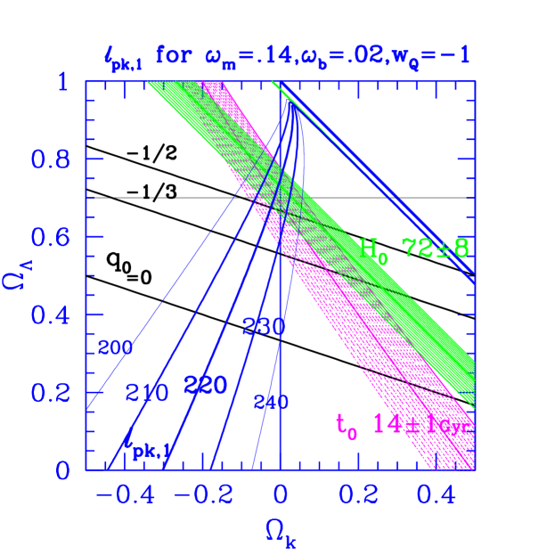
Figure 5: This shows lines of constant $\ell_{pk,1}$ in the $\Omega_{k}$–$\Omega_{Q}$ plane (assuming $w_{Q}$=$-1$, i.e., a cosmological constant) for the $\{\omega_{m},\omega_{b}\}$ shown, near their most probable values. The data give $\ell_{pk,1}=222\pm 3$. The higher peaks and dips have similar curves, scaled about the probable values listed above. Lowering $\omega_{b}$ increases the sound speed, decreasing $\ell_{pk,j}$, and varying $\omega_{m}$ also shifts it. The $0.64<{\rm h}<0.82$ (heavier shading, $H_{0}$) and $13<$ age $<15$ (lighter shading, $t_{0}$) ranges and decelerations $q_{0}=0,-1/3,-1/2$ are also noted. The sweeping back of the $\ell_{pk,j}$ curves into the closed models as $\Omega_{\Lambda}$ is lowered shows that even if $\Omega_{tot}$=1, the phase space results in a 1D projection onto the $\Omega_{tot}$ axis that would be skewed to $\Omega_{tot}>1$. This plot explains much of the structure in the probability contour maps derived from the data, Fig. 6.

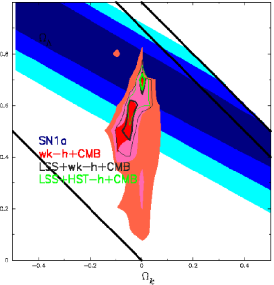
Figure 6: 1,2,3-sigma likelihood contour shadings for “all-data” and the weak-H+age prior probability in the $\Omega_{k}-\Omega_{Q}$ plane. The first interior lines are the 1,2-sigma ones when the LSS constraint is added, the most interior are the contours when the Hubble key project constraint is applied. The supernova contour shadings SN are also plotted. Note that the contours are near the $\Omega_{k}=0$ line, but also follow a weighted average of the $\ell_{pk,1}\sim 220$ lines. This approximate degeneracy implies $\Omega_{Q}$ is poorly constrained for CMB-only, but it is broken when LSS is added, giving a solid SN1-independent $\Omega_{Q}$ ”detection”. When the Hubble key project constraint on $H_{0}$ is added, partial breaking of this degeneracy occurs as well, as is evident from Fig. 5, and from this figure.

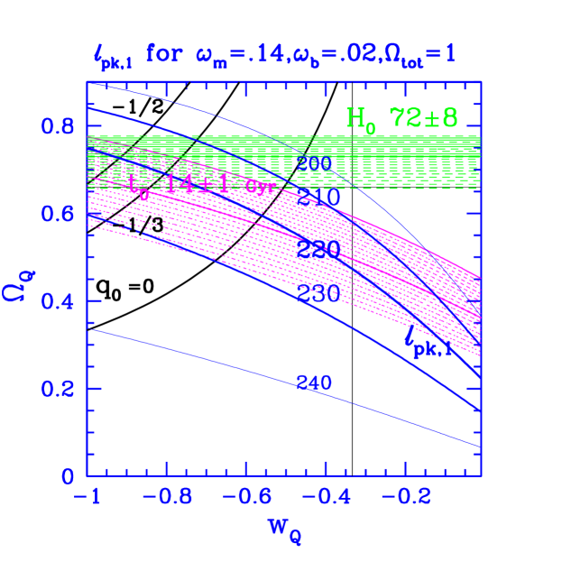
Figure 7: Lines of constant $\ell_{pk,1}$ in the $w_{Q}$–$\Omega_{Q}$ quintessence plane (with $\Omega_{tot}$=1) are shown for the most probable values of $\{\omega_{m},\omega_{b}\}$. Lines of constant deceleration parameter $q_{0}=(\Omega_{m}+(1+3w_{Q})\Omega_{Q})/2$, $H_{0}$ and age $t_{0}$ in the ranges indicated are also shown.

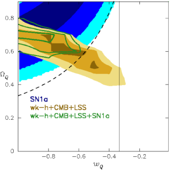
Figure 8: 1,2,3-sigma likelihood contour regions for “all-data” with the weak-H+age prior probability, $\Omega_{tot}$=1, and the LSS prior. 1,2,3-sigma SN1 contour regions perlmutter99 at upper right are rather similar to the constant deceleration lines. The $q_{0}=0$ line is the dashed one. The combined CMB+LSS+SN1 contours are shown as lines. The constraint from CMB on $\Omega_{Q}$ is reasonably good if a strong $H_{0}$ prior (Hubble key project result) is applied, but gets significantly more localized when LSS is added. In neither case is $w_{Q}$ well determined, and $w_{Q}$ localization with CMB+LSS+SN1 is mainly because of SN1. This implies the current limits are not that sensitive to the details of how quintessence impacts low $\ell$ in the DMR regime, which is an uncertainty in the theory.

Marginalized Estimates of our Basic 8 Parameters: Table 1 shows there are strong detections with only the CMB data for $\Omega_{tot}$, $\omega_{b}$ and $n_{s}$ in the minimal inflation-based 8 parameter set. The ranges quoted are Bayesian 50% values and the errors are 1-sigma, obtained after projecting (marginalizing) over all other parameters. With “all-data”, $\omega_{cdm}$ begins to localize, but more so when LSS information is added. Indeed, even with just the COBE-DMR+LSS data, $\omega_{cdm}$ is already localized. That $\Omega_{Q}$ is not well determined is a manifestation of the $\Omega_{k}$–$\Omega_{Q}$ near-degeneracy discussed above, which is broken when LSS is added because the CMB-normalized $\sigma_{8}$ is quite different for open cf. pure $Q$-models. Supernova at high redshift give complementary information to the CMB, but with CMB+LSS (and the inflation-based paradigm) we do not need it: the CMB+SN1 and CMB+LSS numbers are quite compatible. In our space, the Hubble parameter, ${\rm h}=(\sum_{j}(\Omega_{j}{\rm h}^{2}))^{1/2}$, and the age of the Universe, $t_{0}$, are derived functions of the $\Omega_{j}{\rm h}^{2}$: representative values are given in the Table caption. CMB+LSS does not currently give a useful constraint on $w_{Q}$, though $w_{Q}\mathrel{\hbox to0.0pt{\lower 3.0pt\hbox{$\mathchar 536\relax$}\hss}\raise 2.0pt\hbox{$\mathchar 316\relax$}}-0.7$ with SN1. The values do not change very much if rather than the weak prior on ${\rm h}$, we use $0.72\pm 0.08$, the estimate from the Hubble key project Freedman . Indeed just the CMB data plus this restricted range for ${\rm h}$ and the restriction to $\Omega_{tot}=1$ results in a strong detection of $\Omega_{Q}$. Allowing for a neutrino mass mnu changes the value of $\Omega_{Q}$ downward as the mass increases, but not so much as to make it unnecessary.

Table 1: Cosmological parameter values and their 1-sigma errors are shown, determined after marginalizing over the other $6$ cosmological and the various experimental parameters, for “all-data” and the weak prior ($0.45\mathrel{\hbox to0.0pt{\lower 3.0pt\hbox{$-$}\hss}\raise 2.0pt\hbox{$\mathchar 316\relax$}}{\rm h}\mathrel{\hbox to0.0pt{\lower 3.0pt\hbox{$-$}\hss}\raise 2.0pt\hbox{$\mathchar 316\relax$}}0.9$, age $>10$ Gyr). The LSS prior was also designed to be weak. The detections are clearly very stable if extra ”prior” probabilities for LSS and SN1 are included. Similar tables are given in Sievers02 . If $\Omega_{tot}$ is varied, but $w_{Q}=-1$, parameters derived from our basic 8 come out to be: age=$15.2\pm 1.3$ Gyr, ${\rm h}=0.55\pm 0.08$, $\Omega_{m}=0.46\pm.11$, $\Omega_{b}=0.070\pm.02$. Restriction to $\Omega_{tot}=1$ and $w_{Q}=-1$ yields: age=$14.1\pm 0.6$ Gyr, ${\rm h}=0.65\pm.05$, $\Omega_{m}=0.34\pm.05$, $\Omega_{b}=0.05\pm.006$; allowing $w_{Q}$ to vary yields quite similar results.

	cmb	+LSS	+SN1	+SN1+LSS
	$\Omega_{tot}$	variable	$w_{Q}=-1$	CASE
$\Omega_{tot}$	$1.03^{+.04}_{-.05}$	$1.03^{+.03}_{-.04}$	$1.01^{+.07}_{-.03}$	$1.00^{+.07}_{-.03}$
$\Omega_{b}{\rm h}^{2}$	$.022^{+.004}_{-.002}$	$.022^{+.004}_{-.002}$	$.023^{+.005}_{-.003}$	$.023^{+.004}_{-.003}$
$\Omega_{cdm}{\rm h}^{2}$	$.13^{+.03}_{-.03}$	$.12^{+.02}_{-.03}$	$.11^{+.03}_{-.03}$	$.11^{+.03}_{-.03}$
$n_{s}$	$0.94^{+.11}_{-.04}$	$0.93^{+.11}_{-.04}$	$0.97^{+.15}_{-.06}$	$0.99^{+.14}_{-.07}$
$\Omega_{Q}$	$0.53^{+.14}_{-.13}$	$0.57^{+.13}_{-.08}$	$0.70^{+.07}_{-.08}$	$0.70^{+.06}_{-.07}$
	$\Omega_{tot}$	=1	$w_{Q}=-1$	CASE
$\Omega_{b}{\rm h}^{2}$	$.021^{+.003}_{-.002}$	$.022^{+.003}_{-.002}$	$.022^{+.003}_{-.002}$	$.022^{+.003}_{-.002}$
$\Omega_{cdm}{\rm h}^{2}$	$.14^{+.03}_{-.02}$	$.12^{+.01}_{-.01}$	$.12^{+.01}_{-.01}$	$.12^{+.01}_{-.01}$
$n_{s}$	$0.93^{+.05}_{-.03}$	$0.95^{+.09}_{-.04}$	$0.95^{+.09}_{-.04}$	$0.97^{+.08}_{-.05}$
$\Omega_{Q}$	$0.61^{+.09}_{-.38}$	$0.66^{+.05}_{-.06}$	$0.68^{+.03}_{-.05}$	$0.68^{+.03}_{-.05}$
	$\Omega_{tot}$	=1	$w_{Q}$ variable	CASE
$\Omega_{b}{\rm h}^{2}$	$.021^{+.003}_{-.002}$	$.022^{+.003}_{-.002}$	$.022^{+.003}_{-.002}$	$.022^{+.003}_{-.002}$
$\Omega_{cdm}{\rm h}^{2}$	$.14^{+.03}_{-.02}$	$.12^{+.01}_{-.01}$	$.12^{+.01}_{-.01}$	$.12^{+.01}_{-.01}$
$n_{s}$	$0.95^{+.05}_{-.04}$	$0.96^{+.07}_{-.04}$	$0.96^{+.07}_{-.04}$	$0.98^{+.07}_{-.05}$
$\Omega_{Q}$	$0.54^{+.12}_{-.28}$	$0.61^{+.07}_{-.07}$	$0.69^{+.03}_{-.05}$	$0.69^{+.03}_{-.05}$
$w_{Q}$ (95%)	$<-0.43$	$<-0.46$	$<-0.71$	$<-0.71$

The Future, Forecasts for Parameter Eigenmodes: We can also forecast dramatically improved precision with future LDBs, ground-based single dishes and interferometers, MAP and Planck. Because there are correlations among the physical variables we wish to determine, including a number of near-degeneracies beyond that for $\Omega_{k}$–$\Omega_{Q}$ degeneracies , it is useful to disentangle them, by making combinations which diagonalize the error correlation matrix, ”parameter eigenmodes” bh95 ; degeneracies . For this exercise, we will add $\omega_{hdm}$ and $n_{t}$ to our parameter mix, but set $w_{Q}$=$-1$, making 9. (The ratio ${\cal P}_{GW}(k_{n})/{\cal P}_{\Phi}(k_{n})$ is treated as fixed by $n_{t}$, a reasonably accurate inflation theory result.) The forecast for Boomerang based on the 800 sq. deg. patch with four 150 GHz bolometers used is 4 out of 9 linear combinations should be determined to $\pm 0.1$ accuracy. This is indeed what was obtained in the full analysis of CMB only for Boomerang+DMR. The situation improves for the satellite experiments: for MAP, with 2 years of data, we forecast 6/9 combos to $\pm 0.1$ accuracy, 3/9 to $\pm 0.01$ accuracy; for Planck, 7/9 to $\pm 0.1$ accuracy, 5/9 to $\pm 0.01$ accuracy. While we can expect systematic errors to loom as the real arbiter of accuracy, the clear forecast is for a very rosy decade of high precision CMB cosmology that we are now fully into.

References

- (1) Bond, J.R. et al., in “Cosmology & Particle Physics”, Proc. CAPP 2000, ed. J. Garcia-Bellida, R. Durrer, M. Shaposhnikov (Washington: American Inst. of Physics) (2000), astro-ph/0011379
- (2) Mather, J.C. et al., Ap. J. 512, 511 (1999)
- (3) Bond, J.R., Jaffe, A.H. & Knox, L. Ap. J. 533, 19 (2000)
- (4) Bond, J.R., & Jaffe, A., Phil. Trans. R. Soc. London, 357, 57 (1998), astro-ph/9809043
- (5) Miller, A.D. et al., Ap. J. 524, L1 (1999) TOCO
- (6) Mauskopf, P. et al., apjl 536, L59 (2000) BOOM-NA.
- (7) de Bernardis, P. et al., Nature 404, 995 (2000) BOOM00
- (8) Lange, A. et al., Phys. Rev. D 63, 042001 (2001)
- (9) Jaffe, A.H. et al., Phys. Rev. Lett. 86, 3475 (2001)
- (10) Hanany, S. et al., Ap. J. Lett. 545, 5 (2000) Maxima00
- (11) Netterfield, B. et al., Ap. J. 571, 604 (2002) BOOM01
- (12) deBernardis, P. et al., Ap. J. 564, 559 (2002)
- (13) Lee, A.T. et al., Phys. Rev. D 561, L1 (2002) Maxima01
- (14) Ruhl, J. et al., in preparation (2002) BOOM02
- (15) Halverson, N.W. et al., Ap. J. 568, 38 (2002) DASI
- (16) Mason, B. et al., submitted to Ap. J. (2002), astro-ph/0205384 CBIdeep
- (17) Pearson, T.J. et al., submitted to Ap. J. (2002), astro-ph/0205388 CBImosaic
- (18) Seljak, U. & Zaldarriaga, M. Ap. J. 469, 437 (1996) CMBFAST; Lewis, A. Challinor, A., & Lasenby, A. 2000, Ap. J. 538, 473 CAMB, an F90 alternative
- (19) Leitch, E.M. et al., submitted to Ap. J. (2002), astro-ph/0209476; Kovac, J. et al., submitted to Ap. J. (2002), astro-ph/0209478 DASIpol
- (20) Bond, J.R., Jaffe, A.H., & Knox, L., Phys. Rev. D 57, 2117 (1998)
- (21) Myers, S.T. et al., submitted to Ap. J. (2002), astro-ph/0205385
- (22) Sievers, J. et al., submitted to Ap. J. (2002), astro-ph/0205387
- (23) Bond, J.R. et al., submitted to Ap. J. (2002), astro-ph/0205386
- (24) Dawson, K.S., Holzapfel, W.L., Carlstrom, J.E., LaRoque, S.J., Miller, A., Nagai, D. & Joy, M., submitted to Ap. J. (2002), astro-ph/0206012 BIMA
- (25) Bond, J.R. & Crittenden, R.G., in Proc. NATO ASI, Structure Formation in the Universe, eds. R.G. Crittenden & N.G. Turok (Kluwer) (2001), astro-ph/0108204
- (26) Bond, J.R., in Cosmology and Large Scale Structure, Les Houches Session LX, eds. R. Schaeffer J. Silk, M. Spiro & J. Zinn-Justin (Elsevier Science Press, Amsterdam), pp. 469-674 (1996), http://www.cita.utoronto.ca/bond/papers/houches/LesHouches96.ps.gz
- (27) Efstathiou, G. & Bond, J.R., Mon. Not. R. Astron. Soc. 304, 75 (1999). Many other near-degeneracies between cosmological parameters are also discussed here.
- (28) The specific discrete parameter values used for the -database in this analysis were: ( 0,.1,.2,.3,.4,.5,.6,.7,.8,.9,1.0,1.1), ( .9,.7,.5,.3,.2,.15,.1,.05,0,-.05,-.1,-.15,-.2,-.3,-.5) & (0, .025, .05, .075, .1, .15, .2, .3, .5) when –1; ( 0,.1,.2,.3,.4,.5,.6,.7,.8,.9), ( -1,-.9,-.8,-.7,-.6,-.5,-.4,-.3,-.2,-.1,-.01) & (0, .025, .05, .075, .1, .15, .2, .3, .5) when =0. For both cases, ( .03, .06, .12, .17, .22, .27, .33, .40, .55, .8), ( .003125, .00625, .0125, .0175, .020, .025, .030, .035, .04, .05, .075, .10, .15, .2), (1.5, 1.45, 1.4, 1.35, 1.3, 1.25, 1.2, 1.175, 1.15, 1.125, 1.1, 1.075, 1.05, 1.025, 1.0, .975, .95, .925, .9, .875, .85, .825, .8, .775, .75, .725, .7, .65, .6, .55, .5), was continuous, and there were a number of experimental parameters for calibration and beam uncertainties.
- (29) Perlmutter, S. et al., Ap. J. 517, 565 (1999); Riess, A. et al., AJ 116, 1009 (1998)
- (30) Perlmutter, S., Turner, M. & White, M. Phys. Rev. Lett. 83, 670 (1999)
- (31) Freedman, W. et al., Phys. Rep. 568, 13 (2000).
- (32) The simplest interpretation of the superKamiokande data on atmospheric is that , about the energy density of stars in the universe, which implies a cosmologically negligible effect. Degeneracy between e.g., and could lead to the cosmologically very interesting , although the coincidence of closely related energy densities for baryons, CDM, HDM and dark energy required would be amazing.