Parameterization of Dark-Energy Properties: a Principal-Component Approach

Abstract

Considerable work has been devoted to the question of how best to parameterize the properties of dark energy, in particular its equation of state $w$. We argue that, in the absence of a compelling model for dark energy, the parameterizations of functions about which we have no prior knowledge, such as $w(z)$, should be determined by the data rather than by our ingrained beliefs or familiar series expansions. We find the complete basis of orthonormal eigenfunctions in which the principal components (weights of $w(z)$) that are determined most accurately are separated from those determined most poorly. Furthermore, we show that keeping a few of the best-measured modes can be an effective way of obtaining information about $w(z)$.

The discovery of the accelerating universe perlmutter-1999 ; riess has been followed by a lot of work concentrated on how best to parameterize dark energy and measure its properties (huttur ; weller ; maor ; PPF ; SS and references therein). The parameters of choice have been the energy density in this component, $\Omega_{X}$, and its equation-of-state ratio $w(z)$ turner_white . While current data allow interesting constraints only if $w$ is assumed constant, future surveys, such as those envisioned for the Supernova Acceleration Probe (SNAP) SNAP or the Large-aperture Synoptic Survey Telescope (LSST) LSST may allow relaxing that assumption and measuring, for instance, the first derivative of $w$ with redshift, $w^{\prime}\equiv dw/dz|_{z=0}$. Despite these exciting prospects, it has become clear that accurate constraints on a general $w(z)$ will remain elusive even for the most ambitious surveys huttur ; weller ; hence, a simple but general parameterization of $w(z)$ seems necessary.

Yet some issues remain obscure; in particular the question of what is actually being measured by a given survey. In other words, what are the quantitative weights on measurements of $w(z)$? Consider, for example, a fiducial dark-energy model with the equation of state $w(z)=-1+\sin(\pi z)$. Measurements of $w^{\prime}$ would indicate a positive quantity even though the redshift-averaged derivative of $w$ is zero; this is because the largest sensitivity of a measurement is at the low-redshift end where $w^{\prime}(z)>0$. Using somewhat more general arguments, it has been argued huttur ; weller that $w(z)$ is best determined around $z\sim 0.3$, and less accurately determined at much lower and much higher redshift because of the Hubble law and decreasing importance of dark energy respectively. We would like to better understand this and, moreover, find a natural basis of weights that represents the measurement.

We consider the coordinate distance $r(z)$ as the primary observable of any survey (although this could easily be generalized to number-count measurements, for example) and assume a flat universe with energy density in matter $\Omega_{M}=0.3$ and that in the dark component $\Omega_{X}=1-\Omega_{M}$. We divide the redshift range of the survey into $N$ bins centered at redshifts $z_{i}$ with corresponding widths $\Delta z_{i}$ ($i=1,\ldots,N$). We assume dark energy is parameterized in terms of $w(z)$, which we define to be constant in each redshift bin, with a value $w_{i}$ in bin $i$. In the limit $N\rightarrow\infty$, this allows for a completely general $w(z)$. We use $N=50$, which provides sufficient resolution yet doesn’t require large computational time (we have explicitly checked that the results change little for $N\geq 20$). For piecewise-constant $w(z)$, the energy density of the dark component evolves as (for $z$ in bin $j$, $z_{j}-\Delta z_{j}/2<z<z_{j}+\Delta z_{j}/2$)

$$\rho_{X}(z) = \rho_{X}(z=0)\left(\frac{1+z}{1+z_{j}-\Delta z_{j}/2}\right)^{3(1+w_{j})}\times$$ (1)

$$\prod_{i=1}^{j-1}\left(\frac{1+z_{i}+\Delta z_{i}/2}{1+z_{i}-\Delta z_{i}/2}\right)^{3(1+w_{i})}.$$

Then $H^{2}(z)=H_{0}^{2}\,[(1-\Omega_{M})\rho_{X}(z)/\rho_{X}(0)+\Omega_{M}(1+z)^{3}]$ and $H_{0}r(z)=\int H_{0}/H(z^{\prime})dz^{\prime}$. Note that one could use the same methodology to reconstruct other cosmological functions, for example $f(z)\equiv H_{0}/H(z)$.

In this paper, we only consider the function $w(z)$. Although $f(z)$ is easier to measure due to the fact that it is more directly related to the observable luminosity distance, in order to understand the behavior of dark energy, one needs to measure its evolution with time and the scale factor — therefore, measure a derivative of $\rho_{X}(z)$ or $f(z)$. Since $w(z)$ is related algebraically to $df/dz$ reconstr , one effectively needs $w(z)$. Therefore, despite the fact that measurements of $f(z)$ or $\rho_{X}(z)$ will be more accurate than those of $w(z)$, constraints on the latter quantity will be crucial for understanding the nature of dark energy.

We use the Fisher matrix formalism to compute the covariance matrix for the parameters $w_{i}$. We also include the “nuisance parameter” $\mathcal{M}$, which is an overall offset in the magnitude-redshift diagram perlmutter-1999 and $\Omega_{M}$; we then marginalize over these parameters. For the fiducial survey, we assume 3000 type Ia supernovae (SNe) uniformly distributed in redshift between $z=0$ and $z=1.7$. Any actual survey distribution will undoubtedly be somewhat non-uniform in redshift, but we ignore this in order avoid seeing the effects due to the distribution itself.

Figure 1: The principal components of $w(z)$ for $\Omega_{M}$ perfectly known. The four best-determined and two worst-determined eigenvectors are shown and labeled for clarity. We have marginalized over the magnitude offset $\mathcal{M}$.

Principal components of the Fisher matrix.   We start by computing the Fisher matrix $F$ for our parameters $w_{i}$ ($i=1,\ldots,N$), having marginalized over $\mathcal{M}$ and assuming for a moment that $\Omega_{M}$ has been determined independently. We find the familiar result that the accuracy in measurements of $w_{i}$, $\sqrt{(F^{-1})_{ii}}$, rapidly increases with increasing $i$ (that is, redshift). Now, it is a simple matter to find a basis in which the parameters are uncorrelated; this is achieved by simply diagonalizing the inverse covariance matrix (which is in practice computed directly and here approximated with $F$). Therefore

$$F=W^{T}\Lambda W$$ (2)

where the matrix $\Lambda$ is diagonal and rows of the decorrelation matrix $W$ are the eigenvectors $e_{i}(z)$, which define a basis in which our parameters are uncorrelated hamilton . The original function can be expressed as

$$w(z)=\sum_{i=1}^{N}\alpha_{i}\,e_{i}(z)$$ (3)

where $e_{i}$ are the “principal components”. Since $F$ is real and symmetric, $W$ can be chosen to be orthogonal and of unit determinant, so that $\left\{e_{i}(z)\right\}$ form an orthonormal basis. Using the orthonormality condition, the coefficients $\alpha_{i}$ can be computed as

$$\alpha_{i}=\sum_{a=1}^{N}w(z_{a})\,e_{i}(z_{a}).$$ (4)

Diagonal elements of $\Lambda$, $\lambda_{i}$, are the eigenvalues which determine how well the parameters (in the new basis) can be measured; $\sigma(\alpha_{i})=\lambda_{i}^{-1/2}$. We have ordered the $\alpha$’s so that $\sigma(\alpha_{1})\leq\sigma(\alpha_{2})\leq\ldots\leq\sigma(\alpha_{N})$.

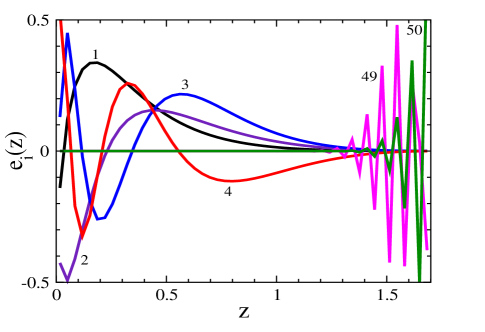
The principal components of $F$ are shown in Fig. 1. For clarity, we only show 4 of the best-determined and 2 of the worst-determined eigenvectors for $w(z)$ for the fiducial model $w(z)=-1$. The best-determined component of $w$ peaks at $z\approx 0.2$, enters with the coefficient $\alpha_{1}=-4.18$, and can be measured to an accuracy of 2.5%. We find that the eigenvectors depend weakly on the fiducial cosmological model, while they depend somewhat more strongly on the set of cosmological parameters; for example, marginalizing further over $\Omega_{M}$ with a prior of 0.03, the best-determined eigenvector of $w$ peaks at $z\approx 0.1$ while the others are mostly unaffected. In addition, allowing that $\Omega_{M}$ is not precisely known increases the uncertainty of how well the first few modes can be measured by 50-100%, while not affecting the higher modes much. Finally, note that, although the best-measured modes peak at relatively low redshifts, one still needs the full redshift range ($z\lesssim 2$) in order to measure those modes accurately.

Note a few nice things about this decomposition (which has recently also been applied to the weak lensing reconstruction of the radial density field hu_keeton ). First of all, the measured eigenvectors are orthonormal and ordered by how accurately they can be measured. The $M^{\rm th}$ best-determined eigenvector has precisely $M-1$ nodes, which makes the interpretation quite natural: the first eigenvector corresponds to the “average of $w(z)$”, the second one to the “first derivative of $w$”, the third one to the “second derivative of $w$”, etc. We argue that, in the absence of a compelling theoretical argument for any particular parameterization of $w(z)$ except perhaps $w(z)\equiv-1$, these modes are the natural basis in which the function $w(z)$ should be considered for any given experiment. Furthermore, the spread in accuracies is larger than before: the best-determined modes are better determined than the best-determined (original) components $w_{i}$, while the worst-determined modes are determined more poorly than the worst-determined $w_{i}$. Of course, the total constraint upon $w(z)$ at any given redshift $z_{a}$

$$\sigma(w(z_{a}))=\left(\sum_{i=1}^{N}\sigma^{2}(\alpha_{i})\,e_{i}^{2}(z_{a})\right)^{1/2}$$ (5)

does not depend on the chosen basis. Consequently, by exploiting only a few of the best-determined modes we might hope to gain in accuracy while not biasing the result too much; we discuss this later on.

A “sweet spot”?   The best-determined eigenvector of $w(z)$ peaks at $z\simeq 0.2$, although other parameter choices (not including the magnitude offset $\mathcal{M}$, for example, or marginalizing over $\Omega_{M}$) can change this to other values, even $z\rightarrow 0$. At first this may seem at odds with the result that $w(z)$ is typically best determined around $z\sim 0.3$ huttur ; weller . However, the question of where the “sweet spot” – the point of minimal uncertainty – of $w(z)$ falls depends on the function which is used to parameterize $w(z)$. For example, using the parameterization $w(z)=w_{0}+w^{\prime}z$ leads to a sweet spot around $z\sim 0.3$. Fitting a low-order polynomial to the distance data may lead to one or two sweet spots in the fitted function huttur ; weller . However, the equation-of-state ratio cannot truly be isolated at a given redshift; moreover, there is no compelling theoretical motivation for any particular parameterization. We therefore argue that the weights we compute are a better representation of the sensitivity of $w(z)$ than the sweet spot in any particular parameterization.

Testing the Constancy of $w(z)$.   The only functional form for $w(z)$ for which, we would argue, there is a strong theoretical bias is a constant $w$, in particular $w(z)=-1$. It is therefore important to test whether the equation of state ratio $w$ is constant or not. Non-constant $w(z)$ would point toward a dynamical mechanism for late-time acceleration of the universe. To test constancy of $w$ one could use actual $r(z)$ data to compare $\chi^{2}$ for models of constant $w(z)$ vs. those of varying $w(z)$. Or one could simply measure $w^{\prime}$ coorayhuterer ; huttur ; weller . Here we seek a more general approach.

Although the $M$th eigenvector $e_{M}(z)$ roughly corresponds to the $(M-1)$th derivative of $w(z)$, it unfortunately cannot be used directly to test the constancy of $w$ simply because the coefficient $\alpha_{M}$ is not zero even for $w(z)={\rm const}$. Now, from Eq. (4) it follows that, for constant $w(z)\equiv w_{c}$

$$\bar{\alpha_{i}}=w_{c}\,\sum_{a=1}^{N}e_{i}(z_{a}).$$ (6)

where $\{\bar{\alpha}_{i}\}$ correspond to the hypothetical $w_{c}$. One can then perform a simple $\chi^{2}$ test to determine whether $w$ is constant:

$$\chi^{2}=\sum_{i=1}^{M}{(\alpha_{i}-\bar{\alpha_{i}})^{2}\over\sigma^{2}(\alpha_{i})},$$ (7)

where we have chosen to keep only the first $M$ eigenmodes, since the best-determined modes will contribute the most to the sum (the test is valid regardless of the value of $M$). Since the best-fitting $w_{c}$ is to be determined by finding the minimum $\chi^{2}$, there are $M-1$ degrees of freedom. For example, for a fiducial model $w(z)=-1.0+0.3\,z$, keeping $M=4$ modes rules out constant $w$ at 98.7% CL. For comparison, the standard $w_{0}$-$w^{\prime}$ test applied to this fiducial model rules out constant $w$ at about $98.5\%$ CL, since $\sigma(w^{\prime})\approx 0.13$. Although the two tests give comparable results, the former describes $w$ with four parameters rather than two and is therefore more general than the $w^{\prime}$ test. In particular, the proposed test has a nice feature that the number of principal components that are used, $M$, can be chosen so as to maximize the strength of the desired constraint.

Function Reconstruction?   From Fig. 1 it is apparent that the well-determined eigenmodes: (1) are non-zero at low end of the redshift range and zero at the high end, and (2) do not oscillate much. The opposite is true for the poorly determined eigenvectors. This tells us that the accuracy in determining $w(z)$ is best if this function is smooth and if we are trying to determine it at low to moderate redshift ($z\lesssim 1$).

We have seen above that the eigenmodes of $w(z)$ are roughly ordered by the absolute size of their coefficients – more noisy modes contribute less to $w(z)$. One can then use the first $M$ eigenvectors (those measured most accurately) in order to approximately reconstruct $w(z)$:

$$w(z)=\sum_{i=1}^{N}\alpha_{i}\,e_{i}(z)\approx\sum_{i=1}^{M}\alpha_{i}\,e_{i}(z)$$ (8)

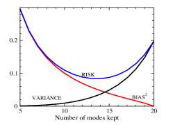
where $M\leq N$. Obviously, in the case of $M=N$ we recover the original error bars, which are typically hopelessly large (at least for $N\gtrsim{\rm few}$, which gives sufficiently high resolution in redshift). When $M<N$, two things happen: $w(z)$ is reconstructed less accurately (so the bias increases), but the error bars are smaller (so the variance decreases). Indeed, getting rid of the noisy eigenmodes corresponds to setting $w(z)$ at high redshift end to zero, which will bias any $w(z)$ that doesn’t actually go to zero at that redshift.

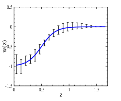
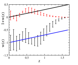
Fig. 2 illustrates these arguments (we choose $N=20$ for definitiveness). To choose the optimal number of eigenmodes to be kept, $M$, the statistically correct thing to do is to minimize risk wasserman , where

$${\rm risk} = {\rm bias}^{2}+{\rm variance}$$ (9)

$$= \sum_{i=1}^{N}\left(w(z_{i})-\bar{w}(z_{i})\right)^{2}+\sum_{i=1}^{N}\sigma^{2}(w(z_{i})),$$ (10)

the sums in Eqs. (3) and (5) run from 1 to $M$, and $\bar{w}$ is the fiducial value of $w$. The top panel of Fig. 2 illustrates the minimization of risk. The bottom left panel of the Figure shows that the fiducial $w(z)=1/2(-1+\tanh(z-0.5))$, which smoothly asymptotes to zero at $z\gtrsim 0.8$, can be reconstructed without much bias; its risk is minimized by keeping $M=4$ terms. The same is not true for $w(z)=-1+0.3\,z$ (bottom right; $M=5$ for minimum bias), which doesn’t go to zero within our redshift range and is therefore reconstructed with a large bias. Furthermore, the reconstructed quantities that are linearly related to $w(z)$, such as $1+w(z)$, will also go to zero at high redshift if $M<N$ (bottom right panel). The resulting bias in $w(z)$ is therefore different for the two cases, and depends on whether $w(z)$ or, say, $1+w(z)$ is reconstructed.

Figure 2: Reconstruction of $w(z)$ by keeping only a fraction of eigenvectors so as to minimize risk. Top panel: illustration of the minimization of risk. Bottom left: optimal reconstruction (68% C.L. error bars shown) of fiducial $w(z)$ (solid line) that goes to zero at high-redshift end. Bottom right: optimal reconstruction of $w(z)$ that does not go to zero at high-redshift end. Also shown on this panel is optimal reconstruction of $1+w(z)$ for the same $w(z)$ model.

This analysis shows that, while reconstructing $w(z)$ at $z\lesssim 1$ is somewhat promising, it does not seem possible to recover $w(z)$ at $z>1$ in a truly model-independent way. We have checked that even adding a large number of SNe at the high-redshift improves the reconstruction only marginally, leaving a significant bias at the high redshift end. The fact that bias (and therefore risk) will be difficult to estimate in practice exacerbates the problem. Note too that the proposed reconstructions of the equation of state ratio reconstr ; huttur ; weller are parametric, since they use a fitting function to fit the distance-redshift data. While planned surveys may provide accurate determinations of the fitting parameters, they cannot test well the validity of the survey parameterization.

Conclusions.   A number of models that roughly explain the observable consequences of dark energy were proposed in recent years, some of them starting from fundamental physics and others being purely phenomenological. However, the origin and nature of dark energy remain unknown, and it is safe to say that none of the models should be taken too seriously at this point. Therefore, it seems wise to approach the question of constraining the properties of dark energy empirically, with as few prior assumptions as possible.

Here we propose that rather than using various parameterizations proposed in the literature to describe dark energy (which typically parameterize the equation of state $w(z)$ using series expansions etc.), one can simply let data decide which weights of these functions are measured best, and which ones are measured most poorly. These weights are the natural basis that parameterizes the measurements of any particular survey.

For definitiveness, we assumed a cosmological distance-redshift survey containing 3000 SNe uniformly distributed in redshift. We computed the weights of $w(z)$ and showed that accurately measured modes (weights) are rather smooth and go to zero at higher redshifts, while the opposite is true for poorly measured modes. The previously-considered “sweet spot” in the sensitivity of $w(z)$ is largely a function of the choice of parameterization, and the shape of the first principal component is a better indicator of the redshift(s) at which $w$ is being measured.

With the proposed parameterization, the test of whether $w(z)$ is constant is straightforward and intuitive. Although the reconstruction of $w(z)$ is straightforward to implement, the reconstructed $w(z)$ is noisy, and it is advantageous to keep only the best-measured modes in order to decrease the statistical reconstruction error. This introduces a systematic bias at $z\gtrsim 1$ for most models, roughly independently of the redshift coverage of SNe. We therefore conclude that while model-independent statements about $w(z)$ at $z\lesssim 1$ may be feasible, those at $z\gtrsim 1$ will be unreliable.

In our opinion, the greatest advantage of this approach is simply having an intuitive and quantitative answer as to what is actually being measured by a given survey. The next logical step is to apply this method to other cosmological tests. We will address this in a future publication.