ALI in Rapidly Expanding Envelopes

Abstract

We discuss the current implementation of the ALI method into our HYDrodynamical RAdiation (Hydra) code for rapidly expanding, low density envelopes commonly found in core collapse and thermonuclear supernovae, novae and WR stars. Due to the low densities, non-thermal excitation by high energy photons (e.g. from radioactive decays) and the time dependence of the problem, significant departures from LTE are common throughout the envelope even at large optical depths.

ALI is instrumental for both the coupling of the statistical equations and the hydrodynamical equations with the radiation transport (RT). We employ several concepts to improve the stability, and convergence rate/ control including the concept of leading elements, the use of net rates, level locking, reconstruction of global photon redistribution functions, equivalent-2-level approach, and predictive corrector methods. For appropriate conditions, the solution of the time-dependent rate equations can be reduced to the time-independent problem plus the (analytic) solution of an ODE For the 3-D problem, we solve the radiation transport via the moment equations. To construct the Eddington tensor elements, we use a Monte Carlo scheme to determine the deviation of the solution for the RT equation from the diffusion approximation (ALI of second kind).

At the example of a subluminous, thermonuclear supernova (SN99by), we show an analysis of the light curves, flux and polarization spectra and discuss the limitations of our approach.

Dept. of Astronomy, University of Texas, Austin, TX 78712, USA

1. Physical and Numerical Environment

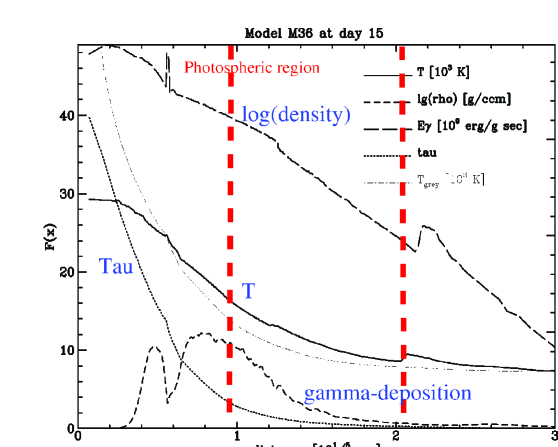
For supernovae, novae and Wolf Rayet stars, detailed hydrodynamical radiation calculations are required to provide a link between the observables such as light curves and spectra, and the underlying physics of the objects. These applications go well beyond classical atmospheres. Density structures require detailed hydrodynamics, the low densities cause strong NLTE effects throughout the envelopes, chemical profiles are depth dependent, the energy source and sink terms due to hydrodynamical effects and radioactive decays may dominate throughout the photon decoupling region, i.e. location of the photosphere and the physical properties are time dependent (see Fig. 1). Typically, velocity fields are of the order of 500 to 30,000 km/sec. Thus, as a major simplification, we can neglect the intrinsic line widths due to pressure broadening, magnetic fields, etc.

Figure 1.: Temperature T, energy deposition due to radioactive decay $E_{\gamma}$, Rosseland optical depth $Tau$ (left scale) and density log($\rho$) (right scale) are given as a function of distance (in $10^{15}cm$) for a typical SNe Ia at 15 days after the explosion. For comparison, we give the temperature $T_{grey}$ for the grey extended atmosphere. The light curves and spectra of Type Ia Supernovae are powered by energy release due to radioactive decay of ${}^{56}Ni\rightarrow^{56}Co\rightarrow^{56}Fe$. The two dotted, vertical lines indicate the region of spectra formation. Most of the energy is deposited within the photosphere and, due to the small optical depth and densities, strong NLTE effects occur up to the very central region (from [Höflich, 1995]).

Figure 2.: Block diagram of our numerical scheme to solve radiation hydrodynamical problems including detailed equation of state, nuclear and atomic networks. For specific problems, a subset of the modules is employed (see text, and Figs. 4 & 5). The code is still under active development. For its current status, see the applications below.

1.1. Numerical Tools and Methods

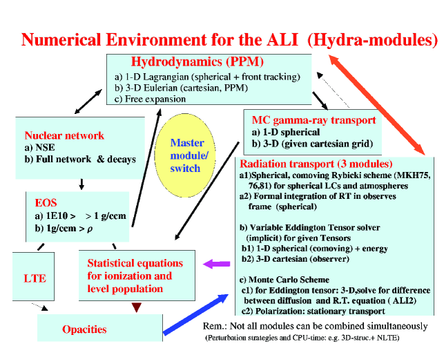
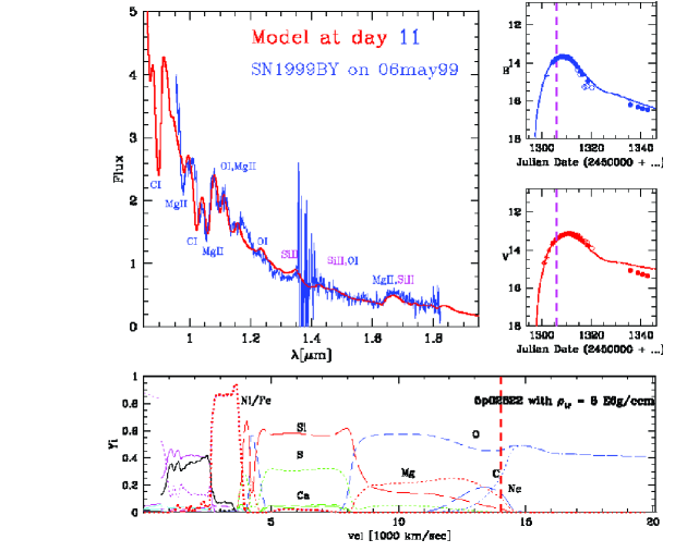
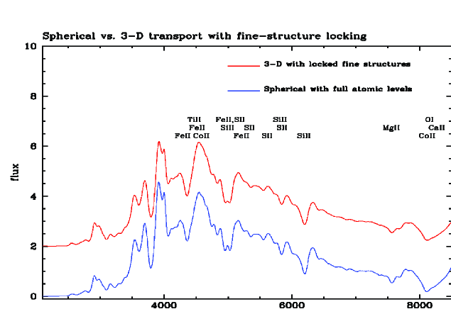
The computational tools summarized below were used to carry out many of the analyzes of SNIa and Core Collapse Supernovae ([Höflich 1988], Höflich, Müller & Khokhlov 1993, [Höflich, 1995], [Howell et al. 2002], …). For the nomenclature we follow Mihalas  & Mihalas (1988) if quantities are not defined explicitly. All components of the codes have been written or adopted in a modular form with well defined interfaces which allows an easy coupling (see Fig. 2 and code verification by exchanging e.g. various radiation transport modules but keeping identical the remaining setup (e.g. Fig. 5). The modules consist of physical units to provide a solution for e.g. the nuclear network, the statistical equations to determine the atomic level population, equation of states, the opacities, the hydro or the radiation transport problem. The individual modules are coupled explicitly. Consistency between the solutions is achieved iteratively by perturbation methods. Currently, not all modules can be combined simultaneously because not all iteration schemes have been implemented and because of requirements on CPU time: a) For full NLTE-spectra with large model atoms and a high frequency resolution we are restricted to the time-independent case based on a given hydrodynamical structure (see Fig. 4) and, for 3-D models, reduced atomic atomic models (level-merging/super-levels) have to be used (Fig. 5. b) Radiation hydrodynamics is restricted to a reduced frequency resolutions with reduced atomic levels (level-merging) and spherical geometry (see Fig. 4. In case of multi-dimensional radiation hydrodynamics, CPU-time requirements restrict applications even further. Currently, we can use of few frequencies to represent the fluxes e.g. in the Lyman and ’Balmer and higher continua’, and 3-level atoms plus spherically symmetric velocity fields for the RT([Höflich, Khokhlov & Wang 2002]), or to the grey case for arbitrary field. Technically, we use the so called ’trivial’ parallelization: Parallelization (via MPI and PVM) is achieved on the module basis, e.g. parallelization of the nuclear network over the grid points, using groups of photons for the Monte-Carlo radiation transport, and sub-domains with ’ghost-cells’ with respect to the spacial and frequency coordinates for the hydro and the comoving frame radiation transport, respectively. In the remainder of this section, we want to describe the various modules.

Hydrodynamics: The structure of the expanding envelopes are obtained by three different modules which by a) assuming free expansion, by solving the hydro equations in b) the Lagrangian frame for spherical geometry including a front tracking scheme to resolve shock fronts (e.g. [Höflich, Wheeler & Thielemann 1998]), or the Eulerian scheme for full 3-D using Cartesian coordinates based on PROMETHEUS ([Fryxell, Arnett & Müller 1991]). The hydro modules use an explicit Piecewise Parabolic Method (PPM) by [Collella & Woodward (1984)] to solve the compressible reactive flow equations. PPM is implemented as a step followed by separate remaps of the thermal and kinetic energy to avoid numerical generation of spurious pressure disturbances during propagation of reaction fronts (flames and detonations).

Nuclear network & high density EOS: Nuclear burning is taken into account using Thielemann’s nuclear reaction-network library ([Thielemann, Nomoto & Hashimoto 1994], and references therein). The main sources for experimental rates are [Caughlan et al.(1985)],[Caughlan & Fowler(1988)] and [Wiescher, Görres & Thielemann (1990)]. Typically, between 20 and 618 isotopes are taken into account. For the equation of state, we use a relativistic Fermi-gas with Coulomb corrections and crystallization, and radiation.

Opacities and low density equation of state: For low densities, we solve the full rate equations (see below) to determine the level population, or assume LTE. Typically, about 500 to 600 discrete NLTE levels are included in full NLTE with about 20,000 to 40,000 line transitions. For the 3-D hydro, the effective number of levels is being reduced by about a factor of 10 by level-merging ([Höflich 1990]), often referred to as the use of super-levels. Complete redistribution over each individual line both in frequency and in angle are assumed. This means that the relative populations within the sublevels or the merged levels are described by a Maxwell-Boltzmann distribution. The data for the atomic line transitions are taken from the new compilation of Kurucz ([Kurucz 1991, Kurucz 1995]) and the opacity project (TOPBASE, e.g. [Cunto & Mendoza 1992]) from which about 500,000 -2,000,000 lines are extracted, depending on the temperature and density range. Photon scattering by free electrons is included in the Klein-Nishina limit. Free-free cross sections are treated in the hydrogen approximation with free-free Gaunt factors according to [Seaton(1960)] and [Gayet(1970)]. Radiative bound-free cross sections are taken from the opacity project (Z$\leq$28).

Gamma-ray transport and energy deposition: The $\gamma$-ray transport is computed in spherical and three-dimensions using a Monte Carlo method (Höflich, Khokhlov & Müller 1992, [Höflich 2002]) including relativistic effects and a consistent treatment of both the continua and line opacities. The interaction processes allowed are: Compton scattering according to the full angle-dependent Klein-Nishina formula, pair-production, and bound-free transitions ([Ambwani & Sutherland 1988], [Brown & Leventhal 1987]).

Radiation transport: Several modules are available. For the spherical geometry and in the stationary case, the radiation transport equation is solved in the comoving frame ([Mihalas, Kunacz & Hummer 1975], [Mihalas, Kunacz & Hummer 1976], [Mihalas, Kunacz & Hummer 1976b], hereafter MKH-methods). For the time dependent cases, we use variable Eddington Tensor solvers (implicit in time) ([Mihalas & Mihalas 1984], [Stone, Mihalas & Norman 1992], [Höflich et al. 1993]). We assume that the Eddington factors are constant during each time step. In the spherical case, we use the MKH methods. To obtain the correct solution for the Eddington tensor elements in 3-D, we use a Monte Carlo method to compute the difference between the solution of the non-equilibrium diffusion and full radiation transport equation. We calculate the difference between the solutions for computational accuracy and efficiency. In particular, the random element in MC avoids spatial fluctuations (and, thus, wiggles) in propagating, plane light fronts though, still, its speed in the free stream limit may differ from the light speed by 5 to 20 %. The same Monte Carlo solver is used which has been applied to compute $\gamma$-ray and polarization spectra for scattering dominated atmospheres (e.g. [Höflich et al. 1992], [Howell et al. 2002]). The Monte Carlo method is appropriate for this problem because of its flexibility with respect to the geometrical and velocity structures.

AutomaticMeshRefinement for radiation transport by a MC torch: Automatic Mesh Refinement is a well established procedure in hydrodynamics and allows to adjust the resolution to the requirements. The same holds true also for radiation transport. In stellar atmospheres, a logarithmic spacing of the optical depth $\tau$ is adopted to guarantee an appropriate resolution. In dynamical problems, extended atmospheres/envelopes with arbitrary morphologies the problem boils down to determine the region of the photosphere, or the ’skin’ of an optically thick object. We start with a grid, equally spaced in mass (in comoving frame) or space (in Eulerian frame), and employ a ’Monte Carlo Torch’ for the grid refinement. As a basic concept, the photosphere is defined as the region from which the photons can escape or, because of the symmetry of the problem, a photon can penetrate to when coming the outside. With the ’torch’, we eluminate the object from the outside and calculate the path of the photons (with various energies) in random directions. If a photon is interacting in a computational cell, we increase its photon counter. Typically, the number of test photons is of the order of the number of cells $n_{R}$ in a grid times the number of representative frequencies $\nu_{rep}$. In our examples (see Figs. 4 & 5), about $10^{6}$ to $10^{7}$ are used both in the spherical ($n_{r}=912$ & $\nu_{rep}=1000$) ) and in the 3-D ($n_{r}\approx 5\times 10^{5}$ & $10\times\nu_{rep}$). Computational cells are divided in half if their photon count exceeds the average by a factor of 5 to 10. By eluminating the object from the edges of the domain, 3-D surfaces will be traced only if they can be seen from the domain boundaries. Concave structures such as the inner edges of Rayleigh Taylor fingers will be missed. Therefore, $\approx 10$ additional photons are emitted from each grid cell. A photon triggers a counter only if it has crossed 2 or more cell boundaries to avoid rezoning of optically thick layers. The requirements of this approach depends on the physical situation. In our examples, we allow for rezoning every 20 to 50 time steps. To test the accuracy, we increase the number of test photons by a factor of 10 about every 10 rezoning steps.

1.2. Accelerated Lambda Iteration & Friends

The radiation field couples the local, statistical equations and the hydro equations, resulting in complex systems of integro-differential equations of rank $DIM=n(x)n(y)n(z)n(\nu)\sum_{el}\sum_{ion(el)}\sum_{level(el,ion)}n(el,ion,level)$ where n(x,y,z) and n$(\nu)$ are the spatial and frequency coordinates, and n(el,ion,level) are the atomic level population of ”level” for element ”el” with the ionization ”ion”. The rank can easily exceed $10^{12...13}$ which prohibits a direct solution. However, the iterative solution provides an effective way to separate global and local quantities.

a) The method of accelerated lambda iteration is used to remove the global dependencies produced by the the radiation field.

b) The statistical equations and the energy terms in the hydro equations are solved by a partial linearization method ([Mihalas & Mihalas 1984]). When evaluating the mean intensity, J_ν, in the rate equations two extreme cases are considered in which the source function of the specific transition does or does not dominate the total source function. This approach further assumes that the variation of the total source function can be represented by the transition under consideration or by the change of the source function during the previous iteration step, respectively. The first case is quite similar to the assumptions of the equivalent two level approximation, but with the difference that the perturbation terms are used instead of the total rates.

c) The concept of “leading” elements is introduced. An appropriate ordering of elements or groups of elements allows a separation of the equations, which are solved by partial linearization. With this technique, the system of equations remains small, independently of the problem. This property is needed to achieve numerical stability and computing efficiency.

d) We use the concept of level-locking ([Höflich 1990]), often called super-levels for numerical efficiency. For stability, we use level locking when the system is far from convergence.

e) The scattering and thermal contributions to the source functions are separated by an equivalent two-level approximation for transitions from the ground levels. In effect, this allows to include the non-local nature of optically thick, scattering dominated transitions already during solution of the full radiation transport problem. In effect, this approach introduces an acceleration term for the convergence of ALI ([Athay 1992], [Avrett & Loeser 1992], [Höflich, 1995]).

f) Based on the explicit forms for the total opacity $\chi(\nu)$ and the source function $S(\nu)$, we reconstruct redistribution functions in $\nu$ for the photon, and limit the relative change between model iterations to $\approx 10\%$.

The accelerated lambda iteration: The intensity I can be obtained by the solution of the radiation transport equation

$${\partial I\over{c\partial t}}+Op~{}I=\chi(S-I)$$ (1)

where $Op=Op(x,y,z,\delta/\delta x,\delta/\delta z,\delta/\delta z,\delta/\delta\nu$, and I is the intensity. On the right hand side, the source function $S$ and and opacity $\chi$ are local quantities.

Formally, the solution of the radiation transport or, better, the first momentum $I$ can be written as $J(x,y,z,\nu)=\Lambda S(x,y,z,t,\delta/\delta x,\delta/\delta y,\delta/\delta z)$, and J can be substituted in the rate and energy equation. The matrix elements $\lambda_{j,i}$ describe the contribution of S at the grid point j on J at the grid point i. In general, $\lambda$ is not constructed explicitly. Instead, it can be approximated by the following expression (e.g. [Cannon 1973], [Scharmer, 1984], [Hillier 1990], [Höflich 1990], [Hubeny & Lanz 1992], [Werner 1991])

$$J_{\nu}^{(m)}=\Lambda_{\nu}^{(m)}S_{\nu}^{(m)}\approx\Lambda_{\nu}^{(m-1)}S_{\nu}^{(m-1)}+\Lambda_{\nu}^{*~{}(m-1)}(S_{\nu}^{(m)}-S_{\nu}^{(m-1)})$$ (2)

and the solution is obtained iteratively where $m$ stands for the iteration step. The first term corresponds to the ’classical’ $\Lambda$ iteration, which works well for low optical depths but the convergence of the $\Lambda$ iteration becomes poor when $\Lambda$ becomes diagonal and if the scattering part is large. The basic idea of the ALI is introduce a second, term which removes the local contribution to the radiation field and drives the convergence. The implementation of the ALI method is reduced to the construction of $\Lambda_{*}$ and the way how the expression for J (eq. 2) is used for the rate and energy equations.

Figure 3.: In expanding envelopes, a photon travels both in the spatial and frequency space from $(r_{o},\nu_{o})$ to $(r_{1},\nu_{1})$ (red arrow). Consequently, any line transition (blue line) $\epsilon[\nu_{o},\nu_{1}]$ will effect the absorption probability of the photon whereas, in the static case, only lines will influence the absorption probability if $|\nu_{line}-\nu_{o}|$ is smaller than the internal line width $\Delta\nu_{line}$. For large velocities, a photon can be absorbed by a given line in small region with almost constant physical properties. This allows for an operator splitting of $Op$ (eq. 1).

Figure 4.: Comparison of a explosion model with the SNe Ia 1999by. We show spectra at day 11 (upper left), the the B and V light curves (right plots), and the chemical structure (lower panel). The explosion and evolution of the spectra are calculates self-consistently with the only free parameters being the initial structure of the exploding White Dwarf, and a parameterized description of the nuclear burning front. The explosion is calculated by a spherical hydro-modules using 912 depth points including a nuclear network with 218 isotopes. After about 10 seconds, only radioactive decays are taken into account but we solve the time-dependent, full NLTE, radiation hydro. The LCs are based on several thousand NLTE-spectra utilizing 912 depth, 2000 $\nu$s and atoms with a total of 50 super-levels. For several moments of time, l, detailed NLTE spectra have been constructed using 90 depth & $\approx 30,000~{}\nu$ points with $\approx 500$ NLTE levels (from [Höflich et al. 2002]).

Figure 5.: Comparison between theoretical spectra for the SNe Ia 1999by at about maximum light assuming spherical symmetry. The spectra are based on our spherical (blue) and full 3-D radiation transport scheme, using 90 depth points, 20,000 frequency points and 520 NLTE-levels and 67/67/67 depth points, 2000 frequency points and 50 NLTE-super-levels, respectively. Differences are up to 20 %. They can be understood due to the lower resolution in the 3-D calculations. As an application, asphericity effects of SN99by (see Fig. 4), see [Howell et al. 2002]).

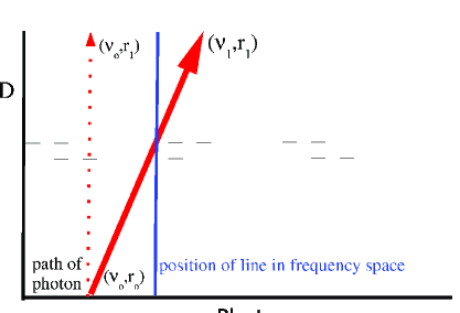
The diagonal operator for rapidly expanding envelopes: In general, the spatial and frequency coordinates are coupled by the radiation transport equation, and the requirements on the corresponding resolutions are linked. In a Rybicki-like scheme for solving the radiation transport equation (e.g. Mihalas et al. 1975), the frequency spatial resolutions must be better the internal lines width, e.g. $\Delta\nu<\nu_{thermal}$, and the velocity difference between two neighboring cells must be $\Delta v<\Delta\nu/\nu*c$ with c being the speed of light. For SN, the velocities are of the order of $10^{4}km/sec$, and the line width are given thermal velocities $v_{therm}\approx 1km/sec$ which requires a $\geq 10,000$ grid points in each direction. However, the extreme ratio between line width and Doppler shift allows for an operator splitting of $Op$ (eq. 1) into a directional and frequency dependent part (see Fig. 3). This allows reduce the solution of the RT problem into the two-stream approximation and to attribute the frequency shift to the opacity which removes the link between the required spatial and $\nu$ resolution.

Expansion opacities: In the presence of large velocity fields, the influence of the lines on the opacities can be well represented in the narrow line limit ([Sobolev 1957], [Castor 1974]) for the given (non-LTE) level populations. We use expressions and presumptions ([Höflich et al. 1993]) very similar to those but but for the comoving frame. The Sobolev opacity of a certain line l between a lower and upper level i and j, respectively, is represented by the expression

$$\chi_{l}={\pi e^{2}\over m_{e}c}{f_{ij}n_{i}\over\nu_{ij}\rho}\Biggl{(}1-{g_{i}n_{j}\over g_{j}n_{i}}\Biggr{)}.$$ (3)

However, the probability to be absorbed by a given line needs to be modified by the probability that a photon did interact before with another line or a continuum. Similar to [Karp et al.(1977)], we obtain the following expression if N scattering lines are ordered with respect to the wavelength

$$\chi_{l}(\nu)=(\sigma_{e}+\chi_{\nu}^{bf}+\chi_{\nu}^{ff})\left[1-\sum^{N_{d}}_{j=J}\left[1-\exp(-\tau_{j})\right](\nu_{j}/\nu)^{s}\exp\left(-\sum_{i=1}^{j-1}\tau_{i}\right)\right]^{-1}$$ (4)

with

$$\tau_{i}=\chi_{i}c\varrho{dr\over dv(r)}~{}~{}and~{}~{}s:=(\sigma_{e}+\chi_{\nu}^{bf}+\chi_{\nu}^{ff})\cdot c\varrho{dr\over d\upsilon}.$$ (5)

Note that the Sobolev optical depth is formulated for a given reference frame. However, we can transform the opacity from frame 0 to the frame of a neighboring grid point by

$$\chi(v/c)=\chi(0)(1.-2{v\over r\chi_{R}(0)})+O(v/c)^{2})\approx\chi(0)$$ (6)

if we assume a linear dependence of $\chi_{\nu}$ in the frequency space and peace-wise linear velocity fields ([Höflich 1990]). Here, $r$ is the local radius of curvature of the velocity field for a direction D. For $\Lambda_{*}$, we can neglect the order O(v/c) in the expression above.

The matrix elements of the $\Lambda_{*}$ operator: We construct $\Lambda_{*}$ in 2-stream approximation, i.e. $Op\rightarrow\delta/\delta D$ and use intensity like variables $u=I^{+}+I^{-}$ for direction D with the grid d. As in static atmospheres ([Olson, Auer & Buchler, 1986]), we obtain

$${\delta I\over\delta d}=\chi(I-S)~{}~{}and~{}with~{}\delta\tau=\chi\delta d\Rightarrow{\delta\over\delta\tau}u=u-S$$ (7)

By using the flux and intensity like variables we get the final equation

$${{u_{d+1}\over\Delta\tau_{d}\cdot\Delta\tau_{d+1/2}}-u_{d}\left({1\over\Delta\tau_{d}\cdot\Delta\tau_{d+1/2}}+{1\over\Delta\tau_{d}\cdot\tau_{d-1/2}}\right)+{u_{d-1}\over\Delta\tau_{d-1/2}\Delta\tau_{d}}}=u_{d}-S_{d}.$$ (8)

with

$$S_{d}=1,u^{*}_{d-1}=u_{d}^{*}\exp\left[-(\tau_{d}-\tau_{d-1})\right],u^{*}_{d+1}=u_{d}^{*}\exp\left[-(\tau_{d+1}-\tau_{d})\right]$$ (9)

$$\chi_{d\pm 1/2}:={1\over 2}\left[\chi_{d\pm 1}+\chi_{d}\right]\Delta\tau_{1+1/2}:=\chi_{d+1/2}\left[z_{d}-z_{d+1}\right],$$ (10)

where $u^{*}_{d}$ is the ”flux” like quantity. After some transformations one gets the algebraic expression

$$\Delta\tau_{d-1/2}:=\chi_{d-1/2}\left[z_{d-1}-z_{d}\right],\Delta\tau_{d+1/2}:={1\over 2}\left[\Delta\tau_{d+1/2}+\Delta\tau_{d-1/2}\right]$$ (11)

$$u^{*}_{d}=\left[1+\left({1-\exp(-\Delta\tau_{d})\over\Delta\tau_{d}\Delta\tau_{d+1/2}}+{1-\exp(-\Delta\tau_{d-1})\over\Delta\tau_{d}\cdot\Delta\tau_{d-1/2}}\right)\right]^{-1}$$ (12)

At the inner boundary of each ray we take for the optically thick and thin cores $u^{*}_{d=d_{max}}=1$ $u^{*}_{d=d_{max}}=(1-e^{-\Delta\tau_{d=d_{max}}})$, respectively. From the the known u${}_{d}^{*}$ we get the diagonal element by

$$\Lambda_{\nu}^{*}=\int\limits^{*}_{0}d\mu d\phi u^{*}_{d}.$$ (13)

One remaining problem related to the property that the locality of the operator depends on the resolution, i.e. the convergence rate becomes grid dependent and, for high resolutions, the system may become unstable. The information on corrections propagates only one grid point per model interaction m. To overcome these problems and if the solution is far from convergence, we refine the the ’grid/average over several zones’ corresponding to the thermalization depth $\tau_{therm}$ of the transition with the highest opacity of a given element. The estimate of $\tau_{therm}$ based on the equivalent-two-level approach. Successively, we increase the effective resolution to the full grid resolution. For our applications, this approach has been found to be more stable rather than using off-diagonal elements ([Werner 1991]) but, in light of discussions at this meeting, the latter approach will be revisited.

The matrix elements of the statistical equations: The matrix elements of the statistical equation A x = b of each species are given by

$$A_{ij}=\cases{-(R_{ij}+C_{ij})&$i<j$\cr-({n_{i}^{*}\over n^{*}_{j}})(R_{ji}+C_{ij})&$j>i$\cr\sum^{i-1}_{l=1}({n_{l}^{*}\over n_{i}^{*}})(R_{il}+C_{il})+\sum^{n}_{l=i+1}(R_{il}+C_{il})&$j=i$\cr}$$ (14)

$R_{ij}$ and $C_{ij}$ are the radiative and collisional rates relating the levels i and j.

The radiative rates between a lower and upper level i and j, respectively, are given by

$$R_{ij}=4\pi\int{\alpha_{ij}(\nu)\over h\nu}J_{\nu}d_{\nu}+R(\gamma-rays)$$ (15)

$$R_{ji}=4\pi\int{\alpha_{ij}(\nu)\over h\nu}\left[{2h\nu^{3}\over c^{2}}+J_{\nu}\right]e^{-{h\nu\over kT}}d\nu.$$ (16)

Here, where the coupling between the radiation field and the statistical equations occurs, in principle, the solution of the statistical equations of the current model iteration (m) has to be known in order to calculate the new value of the radiation field $J_{\nu}^{(m)}$. In order to estimate the updated rates, we distinguish two cases:

Case A: $S_{\nu}/\chi_{\nu}\gg S_{ij}/\chi_{ij}$ and B) $S_{\nu}/\chi_{\nu}\approx S_{ij}/\chi_{ij}$. Case A: Eqs. 15 and 16 can be written as a sum of the ”zero” order

$$R_{ij}=4\pi\int{\alpha_{ij}(\nu)\over h\nu}\Lambda_{\nu}S_{\nu}^{(m-1)}d\nu$$ (17)

$$R_{ji}=4\pi\int{\alpha_{ij}(\nu)\over h\nu}\Biggl{[}{2h\nu^{3}\over c^{2}}+\Lambda_{\nu}S^{(m-1)}_{\nu}\Biggr{]}e^{{-h\nu\over kT}}d~{}\nu d\nu$$ (18)

and by correction terms of ”first” order

$$R_{ij}^{corr}=4\pi\int{\alpha_{ij}(\nu)\over h\nu}\Lambda_{\nu}^{*}(S^{(m)}_{\nu}-S^{(m-1)}_{\nu})d\nu$$ (19)

$$R_{ji}^{corr}=4\pi\int{\alpha_{ij}(\nu)\over h\nu}\Lambda_{\nu}^{*}(S^{(m)}_{\nu}-S^{(m-1)}_{\nu})e^{{-h\nu\over kT}}d~{}\nu$$ (20)

In order to estimate the source functions we use again the concept of the ”leading” elements. If the total emissivity at the considered frequency is dominated by an element which is higher in the hierarchy, the new difference between the old and the new source function is substituted by the difference of the dominating transitions (marked by the index dom), i.e.

$$(S_{\nu}^{(m)}-S_{\nu}^{(m-1)})\approx(S_{dom}^{(m)}-S_{dom}^{(m-1)})\cdot\chi_{dom}/\chi_{\nu}.$$ (21)

Otherwise the monochromatic source function is just an extrapolation in the second order of the iteration steps, i.e.

$$\Delta S_{\nu}^{(m)}\simeq\Delta S_{\nu}^{(m-1)}+{\Delta S^{(m-2)}-\Delta S^{(m-1)}\over 2}+...$$ (22)

with

$$\Delta S_{\nu}^{(m)}:=S_{\nu}^{(m)}-S_{\nu}^{(m-1)}.$$ (23)

Case B: If the transition in consideration dominates the total source function, we use the approach $S_{\nu}\approx S_{ij}(\nu).$ In order to get expressions for the ”first” order corrections to the rates, essentially, using the same assumptions as in the case of the equivalent two level approach. The explicit forms of the source functions allow us to substitute the departure coefficient of the lower level in the rate equations (e.g. Pauldrach 1987). After some simple transformations, one ends up with the expression for the first order correction of the rates

$$R_{ij}^{corr}=0~{}~{}~{}and~{}~{}~{}R_{ji}^{corr}=4\pi\int{\alpha_{ij}(\nu)\over h\nu}\Lambda_{ij}^{*}(\nu){(S_{ij}^{(m-1)}(\nu)-S^{(m)}_{ij}(\nu))\over S_{ij}^{(m)}(\nu)}d\nu$$ (24)

The separation between the cases A and B is needed to overcome numerical instabilities during the model iteration. The rate equations and the hydrodynamics are iteratively coupled via the energy equation (e.g. [Höflich et al. 1993]). For $J$, we use the same expressions and case separation as just outlined.

1.3. The Time-dependent Rate Equations

An approximate solution of the time dependent non-LTE problem is outlined ([Höflich 1991b]). The statistical equations are reduced to a form of time independent equations which can be solved by one of the standard methods for the time independent case, where the time dependent quantities enter the statistical equations just in an additional explicit rate. These are calculated analytically solving a linear inhomogeneous differential equation of first order.

We assume that the time dependence is caused by a limited number of transitions. In our implementation, we assume that the time dependence is caused by the bound-free transitions. This condition is valid as long as forbidden transitions are suppressed because allowed bound-bound transitions are faster than bound-free transitions by orders of magnitude. This limits the applicability e.g., for SNeIa, to times $\leq$ 40 to 60 days after the explosion. Forbidden lines causes the discrepancies in the late LCs in Fig. 4.

In general, the time dependent rate equations are given by the expression

$${\partial n_{i}\over\partial t}+\nabla(n_{i}\underline{v})=\sum_{i\neq j}(n_{j}P_{ji}-n_{i}P_{ij})+n_{k}(R_{ki}+C_{ki})-n_{i}(R_{ik}+C_{ik})$$ (25)

where the rate P_ij is the sum of radiative and collisional processes.

The time independent solution $\tilde{n}_{i}$ of the statistical equations is defined by the equations

$$0=\sum_{i\neq j}(\tilde{n}_{j}P_{ji}-\tilde{n}_{i}P_{ij})+\tilde{n}_{k}(R_{ki}+C_{ki})-\tilde{n}_{i}(R_{ik}+C_{ik})$$ (26)

that can be solved by a standard method.

For most astrophysical applications, the time scales of allowed bound-bound transitions are much shorter than those of the bound-free transitions, and we obtain the relation

$$\Rightarrow{n_{i}\over n_{j}}={\tilde{n}_{i}\over\tilde{n}_{j}}.$$ (27)

Subtracting the time independent rate equations from the time dependent ones both of which are normalized to $n_{i}$ and $\tilde{n}_{i}$, respectively, results in

$${\partial n_{i}\over\partial t}+{\partial\over\partial r}(n_{i}v(r))=n_{k}(R_{ki}+C_{ki})-{\tilde{n_{k}}\over\tilde{n_{i}}}(R_{ki}+C_{ki})~{}n_{i}$$ (28)

i.e. an inhomogeneous linear differential equation of first order

$$\Rightarrow{dn_{i}\over dt}=-C_{1}n_{i}+C_{2}$$ (29)

with

$$C_{1}:={\tilde{n_{k}}\over\tilde{n_{i}}}(R_{ki}+C_{ki})~{}~{}and~{}~{}C_{2}:=n_{k}(R_{ki}+C_{ki}).$$ (30)

This inhomogeneous ODE is solved analytically as an initial boundary problem. If more than two ionization stage are important, we end up with a system of ODEs to be solved numerically. $n_{k}$ and $\tilde{n_{k}}$ are determined iteratively by using charge conservation in a simple fix point iteration, or a Newton-Raphson method.

Acknowledgments.

This research is supported in part by NASA Grant LSTA-98-022.

References

- Ambwani & Sutherland 1988 Ambwani, K., Sutherland, P.G. 1988, ApJ 325, 820
- Athay 1992 Athay R. 1972 Radiation Transport in Spectral Lines, Reidel Publ.C., Dordrecht
- Avrett & Loeser 1992 Avrett G., Loeser R. 1992, 7th Cambridge Workshop on Cool Stars, ASP Conference Series 26, 489
- Brown & Leventhal 1987 Brown, B.L., Leventhal, M. 1987, ApJ 319, 637
- Cannon 1973 Cannon C.J, 1973, JQSRT 13, 627
- Castor 1974 Castor, J.I. 1974, MNRAS 169, 279
- Caughlan et al.(1985) Caughlan G.R , Fowler A.M., Harris M.J., Zimmerman B.A. 1985, At. Data Nucl. Dat a Tables 32, 197
- Caughlan & Fowler(1988) Caughlan G.R , Fowler A.M. 1988, Atomic Data Nucl. Table, 40, 283
- Collella & Woodward (1984) Colella, P., Woodward, P.R. 1984, J.Comp.Phys. 54, 174
- Cunto & Mendoza 1992 Cunto, W., Mendoza, C. 1992 Topbase, IBM Venezuela Scientific Center
- Fryxell, Arnett & Müller 1991 Fryxell B., Arnett D., Müller E. 1991, ApJ 367, 619
- Gayet(1970) Gayet R. 1970, A&A 9, 312
- Hillier 1990 Hillier D.J. 1990, A&A 231, 116
- Höflich 2002 Höflich, 2002, New Astronomy, in press
- Höflich et al. 2002 Höflich, P., Gerardy, C. L., Fesen, R. A., & Sakai, S. 2002, ApJ, 568, 791
- Höflich, Khokhlov & Wang 2002 Höflich, P., Khokhlov A.M., , Wang L. 2002, in: Texas Converence on Relativistic Astrophysics, eds. Wheeler & Martel, AIP Conference Proceedings 586, p. 459
- Höflich, Wheeler & Thielemann 1998 Höflich, P., Wheeler, J. C., and Thielemann, F.K. 1998, ApJ 495, 617
- Höflich, 1995 Höflich, P. 1995, ApJ 443, 89
- Höflich et al. 1993 Höflich, P., Mueller, E., & Khokhlov, A. 1993, A&A, 268, 570
- Höflich et al. 1992 Höflich, P., Khokhlov, A., & Mueller, E. 1992, A&A, 259, 549
- Höflich 1991 Höflich, P. 1991 A&A 246, 481
- Höflich 1991b Höflich, P. E. 1991b, in ESO-Workshop on Supernovae, Elba, September 1990, ed. J. Danziger et al., p. 387
- Höflich 1990 Höflich, P. 1990, A quantitative analysis of type II supernovae atmospheres, thesis submitted in partial fulfillment of the conditions for admission to the degree of Dr.rer.nat.habil., U München, MPA 563
- Höflich 1988 Höflich, P. 1988, PASP 7, 434
- Howell et al. 2002 Howell, D. A., Höflich, P., Wang, L., & Wheeler, J. C. 2001, ApJ, 556, 302
- Hubeny & Lanz 1992 Hubeny I., Lanz T. 1992, A&A 262, 501
- Karp et al.(1977) Karp, A.H., Lasher, G., Chan, K.L., Salpeter E.E. 1977, ApJ 214, 161
- Kurucz 1995 Kurucz R.L. 1995, CD-23, Center for Astrophysics
- Kurucz 1991 Kurucz R.L. 1991, CD-1, Center for Astrophysics
- Lang 1974 Lang, C. 1974 Astrophysical formulae, Springer Press, Berlin/Heidelberg/ New York Wiley, New York, p.162ff
- Mihalas & Mihalas 1984 Mihalas, D. & Mihalas, B. W. 1984, ’Foundation of Radiation Hydrodynamics’, New York, Oxford University Press
- Mihalas, Kunacz & Hummer 1975 Mihalas D., Kunasz R.B., Hummer D.G. 1975
- Mihalas, Kunacz & Hummer 1976 Mihalas D., Kunasz R.B., Hummer D.G. 1976
- Mihalas, Kunacz & Hummer 1976b Mihalas D., Kunasz R.B., Hummer D.G. 1976b
- Olson, Auer & Buchler, 1986 Olson G.L., Auer L.H., Buchler J.R. 1986, JQSRT 35, 431
- Pauldrach 1987 Pauldrach P. 1987, A&A 183, 295
- Scharmer, 1984 Scharmer G.B. 1984, in Methods of Radiative Transfer, ed. Kalkofen, Cambridge University Press, London
- Seaton(1960) Seaton M.J. 1960, Rep. Prog. Phys. 23, 313
- Sobolev 1957 Sobolev V.V. 1957, Sov. Astron.J. 1, 297
- Stone, Mihalas & Norman 1992 Stone, J. M., Mihalas, D., & Norman, M. L. 1992, ApJS, 80, 819
- Swings 1988 Swings J.P (editor), 1988, in: Transactions of the IAU, Vol. XX A, Kluwer, Dordrecht
- Thielemann, Nomoto & Hashimoto 1994 Thielemann F.-K., Nomoto K., Hashimoto M. 1994, in: Supernovae, Les Houcheseds. S. Bludman R., Mochkovitch J., Mochkovitch J., Zinn-Justin, Elsevier, Amsterdam, p 629
- Werner 1991 Werner K. 1991, A&A 251, 147
- Wiescher, Görres & Thielemann (1990) Wiescher M., Görres J., Thielemann, F.K. 1990, ApJ 363, 340