Correcting for lensing bias in the Hubble diagram

Gravitational lensing will cause a dispersion in the Hubble diagram for high redshift sources. This effect will introduce a bias in the cosmological parameter determination using the distance-redshift relation for Type Ia supernovae. In this note we show how one can diagnose and correct for this bias when doing precision cosmology with supernovae.

1 Introduction

During the last decade, gravitational lensing has become one of the most important tools in cosmology. Weak lensing measurements are used to obtain information on the amount and distribution of matter in the universe (see, e.g., van Waerbeke et al., 2001; Hennawi et al., 2001). Strong lensing has long been recognized as a tool to constrain cosmological parameters (see, e.g., Koopmans & Fassnacht, 1999; Browne, 2000, for measurements of the Hubble constant, $H_{0}$). Controversial upper limits on the amount of dark energy have been derived from the statistics of multiply imaged quasars and radio sources (Kochaneck, 1996; Falco et al., 1998). Using a different set of Schechter parameters for E/S0 galaxies Chiba & Yoshii (1999) conclude that the same quasar data set is best fitted with a universe dominated by dark energy, i.e., in agreement with the concordance cosmology, $(\Omega_{\rm M},\Omega_{X})=(0.3,0.7)$ whereas Keeton (2002) argue that when calibrated to counts of distant galaxies, the method loses most of its sensitivity to the amount of dark energy.

Further, in Goobar et al. (2002b) it is shown how one could use multiple images of supernovae (SNe) to simultaneously measure $H_{0}$, the fractional energy density components and the equation of state parameter of a possible dark energy component. The classical SN cosmological test however, is to study the distance-redshift relation using Type Ia SNe as standard candles. The effect of gravitational lensing on these measurements is to cause an additional dispersion in the observed magnitudes and thus be a source of systematic error in the cosmological parameter determination (see e.g. Wambsganss et al., 1997; Mörtsell et al., 2001b). In this note we show how the negligence of this effect may lead to a systematic underestimation of $\Omega_{\rm M}$. We also investigate how this bias can be diagnosed and corrected for by using the correct probability distribution function (pdf) for the dispersion in SN magnitudes.

In Sects. 2 and 3 we discuss the method and the numerical simulations used in the analysis. In Sect. 4, we investigate what kind of bias we expect if not taking lensing effects into consideration, i.e., assuming a Gaussian magnitude distribution. In Sect. 6, the dispersion in magnitudes due to gravitational lensing is parametrized for different matter distributions and redshifts and in Sect. 7 we correct for lensing effects by performing a maximum likelihood (ml) analysis using the correct pdf’s.

2 The distance-redshift cosmological test

The distances and redshifts of Type Ia SNe can be used to fit, e.g., the mass energy density, $\Omega_{\rm M}$, and the dark energy density, $\Omega_{X}$, in a Friedmann-Lemaître universe. The relation between the parameters can be expressed as

$$m(\@vec{\theta},{\cal M},z) = {\cal M}+5\log_{10}\left[d^{\prime}_{L}(\@vec{\theta},z)\right]\,,$$ (1)

$${\cal M} = 25+M+5\log_{10}(c/H_{0})\,,$$ (2)

where $\cal M$ is a nuisance parameter containing the absolute magnitude, $M$, of the SNe and $H_{0}$ is the Hubble constant. Here $\@vec{\theta}$ represents the parameter vector $\@vec{\theta}=(\Omega_{\rm M},\Omega_{X},w)$. Further the luminosity distance $d^{\prime}_{L}$ is given by

$$d^{\prime}_{L} = \left\{\begin{array}[]{ll}(1+z)\frac{1}{\sqrt{-\Omega_{k}}}\sin(\sqrt{-\Omega_{k}}\,I)\,,&\Omega_{k}<0\\ (1+z)\,I\,,&\Omega_{k}=0\\ (1+z)\frac{1}{\sqrt{\Omega_{k}}}\sinh(\sqrt{\Omega_{k}}\,I)\,,&\Omega_{k}>0\\ \end{array}\right.$$ (6)

$$\Omega_{k} = 1-\Omega_{\rm M}-\Omega_{X}\,,$$ (7)

$$I = \int_{0}^{z}\,\frac{dz^{\prime}}{H^{\prime}(z^{\prime})}\,,$$ (8)

$$H^{\prime}(z) = \sqrt{(1+z)^{3}\,\Omega_{\rm M}+\Omega_{X}(1+z)^{3(w+1)}+(1+z)^{2}\,\Omega_{k}}\,.$$

The usual way to proceed is to make a $\chi^{2}$-fit of $(\Omega_{\rm M},\Omega_{X},\cal M)$ using Eq. (1) assuming that the dispersion in magnitudes is Gaussian distributed (as the intrinsic dispersion of Type Ia SNe seems to be). The same procedure can be used to fit, e.g., the equation of state parameter, $w$, of a more general dark energy component (Goliath et al., 2001).

Gravitational lensing will however induce an asymmetry in the magnitude distribution and in order to avoid a bias in the cosmological parameter estimation, we need to perform a ml-analysis with the correct pdf.

3 Simulated data sets

We use the numerical simulation package, SNOC, the SuperNova Observation Calculator (Goobar et al., 2002a), to obtain simulated samples of the intrinsic dispersion and gravitational lensing effects of Type Ia SNe. The intrinsic dispersion and measurement error is represented by a Gaussian distribution with $\sigma_{m}=0.16$ mag. Gravitational lensing effects are calculated by tracing the light between the source and the observer by sending it through a series of spherical cells in which the dark matter distribution can be specified.

We model compact dark matter as point masses and smooth dark matter with the Navarro-Frenk-White [nfw; Navarro et al. (1997)] density profile using halo parameters, mass distributions and number densities as outlined in Bergström et al. (2000). Note that the results obtained in this paper are not sensitive to the exact parameterization of the smooth halo profile. Also, the results are independent of the individual masses of the compact objects as well as their clustering properties on galaxy scales (Holz & Wald, 1998; Bergström et al., 2000). Any eventual small subhalo structure in the dark matter halos does not act as a compact component (Mörtsell et al., 2001a).

Two different types of simulated data sets have been used for the analysis presented in this note. The first one, A, assumes that the number of observed Type Ia SNe is constant per comoving volume, which means that the number of events increases rapidly for higher redshifts. The B distribution instead assumes a constant number of SNe per redshift interval, i.e., a uniform $z$-distribution. Each data set consists of 2000 SNe in the redshift interval $0.01<z<2.0$.

The number 2000 corresponds roughly to one year’s data from the proposed satellite telescope Supernova/Acceleration Probe [snap; Perlmutter et al. (2000)]. The exact redshift distribution of the Type Ia SNe to be followed by snap is the subject of several ongoing science and instrumental optimization studies. The current anticipated distribution is roughly a constant rate per comoving volume for $z<1$ and a uniform distribution at higher redshifts. In that respect is the A distribution to be regarded as a limiting case of maximal lensing effects due to the large number of high redshift SNe.

To each of these data sets, 300 SNe between $0.04<z<0.08$ have been added. These numbers correspond to the predicted results from the Supernova Factory Campaign (Aldering, Supernova Factory Webpage, ) that is scheduled to start in 2003. Since lensing effects get larger at higher redshifts, the magnitudes of theese SNe are unaffected. For example, for a supernova at redshift $z=0.08$ the lensing effects are in general of the order of 0.01 magnitudes for a dark matter model where the fraction of compact objects is assumed to be 20 %.

All simulations have been made assuming a universe with $\Omega_{\rm M}=0.3$, $\Omega_{X}=0.7$, $w=-1$ and $H_{0}=65$ km s${}^{-1}\,$Mpc^-1.

4 The $\chi^{2}$-fit of cosmological parameters

Making a $\chi^{2}$-fit of $(\Omega_{\rm M},\Omega_{X},\cal M)$ using Eq. (1) (assuming $w=-1$) will for the data set B, described in Sect. 3, result in the solid contour presented in Fig. 1(a) if lensing effects are absent.

(a) Fits in the $(\Omega_{\rm M},\Omega_{X})$-plane.

(b) Fits in the $(\Omega_{\rm M},w)$-plane assuming a flat universe.

Figure 1: Confidence contours showing the 1.51 $\sigma$ level, i.e., the  68 % level for two parameters, for three-parameter $\chi^{2}$-fits where the third parameter $\cal M$ is treated as a nuisance parameter. All fits are based on a simulated sample of 2300 SNe according to the data set B, but different gravitational lensing models have been considered. The dashed contours show the fit when a nfw halo model has been applied, and the dotted and dash-dotted contours represent different fractions of compact objects (c.o.) in the dark matter model.

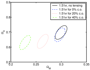
If lensing dispersion is added, the fits of the cosmological parameters will be biased in accordance with the figure. All contours show the $1.51\,\sigma$ level, which corresponds to a $\sim 68\,\%$ confidence region of including the true value of the two parameters.

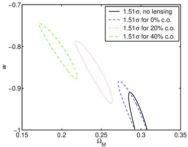
The amount of bias depends on the matter distribution responsible for the lensing effects. The dashed contour shows the result if only a nfw halo model is considered, while the dotted (dash-dotted) contour is based on a simulation where the fraction of compact objects in the dark matter model is 20 % (40 %).

Fig. 1(b) shows similar fits for the $(\Omega_{\rm M},w)$-plane where a flat universe is assumed $(\Omega_{X}=1-\Omega_{\rm M})$. $\cal M$ is still treated as a nuisance parameter, i.e., no prior knowledge is assumed. Also this figure is based on the data set B, but using the A distribution does not significantly alter the qualitative nature of the results. Gravitational lensing starts to become important for $z>1.0$, and in the interval $1.0<z<2.0$, the distributions A and B are quite similiar.

In Fig. 1(b) it is evident how important it is to consider lensing effects since a naive analysis of lensed data may in fact misleadingly exclude a cosmological constant as the explanation for the dark energy.

The size of the bias, i.e., the systematic errors due to lensing in the above figures depends on the asymmetry of the magnitude distribution, which is described in Sect. 5. This in turn depends on the redshift for a given dark matter model. The statistical error – the sizes of the ellipses – on the other hand only depend on the sample size so it is interesting to see where these two errors are comparable.

In Fig. 2 the solid curve is the estimated statistical error of $\Omega_{\rm M}$ plotted as a function of the sample size. It should be noted here that zero events means zero events from the high-$z$ distribution, whereas the 300 events from the Supernova Factory simulations are always present.

Figure 2: The evolution of the systematic error due to gravitational lensing for different dark matter models and the statistical error (the solid curve) as a function of the sample size. Note that zero SNe correspond to zero high-$z$ events, i.e., the fits are only based on the 300 low-$z$ events that are always added. The scatter in the lensing bias curves illustrates the stochastic nature of the effect: a handful of high-magnification supernovae may produce large effects in the fitted cosmological parameters.

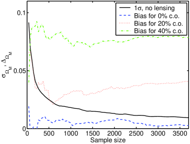
It is interesting to note in this figure that the full data set of 2300 SNe is not necessary to get systematic errors comparable to the statistical error, but gravitational lensing has to be considered also for rather small data samples containing high redshift SNe ($z\raise 1.29167pt\hbox{$>$}\kern-7.5pt{\lower 2.79857pt\hbox{$\sim$}}1$) if the fraction of compact objects is non-negligible.

5 Determining the lensing dispersion

As we have seen, gravitational lensing may induce sizeable systematic effects when trying to determine cosmological parameters using the distance-redshift relation for standard candle sources. A virtue of gravitational lensing is however that the distribution of luminosities can be used to obtain information on the matter distribution in the Universe, e.g., to determine the fraction of compact objects like primordial black holes or MACHOs.

As shown in Mörtsell et al. (2001a), gravitational lensing effects are quite similar for different smooth dark matter halo distributions, but very sensitive to the fraction of the matter density in compact objects, $f_{\rm p}$. Assuming that the major part of the matter density in the universe is in either smooth halos or compact objects, we can thus parametrize lensing effects with $f_{\rm p}$.

Using SNOC, large data sets of synthetic SN observations over a broad redshift range were created with a variable fraction of compact objects ranging from 0 to 40 %, see Fig. 3.

Figure 3: Magnitude dispersion of data set B for 0 % (full line), 20 % (dashed line) and 40 % (dotted line) compact objects using logarithmic scale. The bottom panel includes a Gaussian smearing, $\sigma_{m}=0.16$ mag, due to intrinsic brightness differences between SNe and from measurement error.

Using the Kolmogorov-Smirnov test, it was shown how the matter density in compact objects can be determined using SN data comparable to set A or B to $<5$ % accuracy which we will assume to be the predicted uncertainty in the parameter $f_{\rm p}$, see also Metcalf & Silk (1999) and Seljak & Holz (1999). We now want to parametrize the magnitude distributions obtained from the Monte-Carlo simulations to obtain approximately correct pdf’s to be used in the ml-analysis.

6 Parametrizing the pdf

We parametrize the pdf’s for different fractions of compact objects and redshifts with a Gaussian with a high magnification tail, i.e.,

$$f(m) = a\cdot e^{-\frac{(m-m_{0})^{2}}{2\sigma^{2}}},\quad m>m_{\rm c}$$

$$f(m) = a\cdot e^{-\frac{(m-m_{0})^{2}}{2\sigma^{2}}}+b\cdot|m|\cdot 10^{s\cdot m},\quad m<m_{c}.$$ (9)

This distribution is motivated by the fact that the dominating intrinsic Gaussian dispersion will be shifted toward fainter values since a majority of lines-of-sight contain less matter than in a Friedmann-Lemaître universe. The tail represents the effect of, e.g., galaxies lying close to some lines-of-sight causing high magnifications.

We can set $s=1.5$ and $m_{c}=0$ for all cases and still have a reasonable $\chi^{2}$. Since the fitted probability density functions are normalized to give an integrated probability of unity before performing the maximum likelihood analysis, our parameters are $m_{0},\sigma$ and $b/a$.

As an example, see Fig. 4, where Eq. (6) is fitted to a reference sample corresponding to 40 000 sources at $z=1$ in a universe with a 15 % mass fraction in compact objects. Here, $m_{0}=0.01756,\sigma=0.1653$ and $b/a=0.02530$ with $\chi^{2}/{\rm ndf}=86.44/68$.

Figure 4: Fitting Eq. (6) to the reference sample corresponding to 15 % compact objects. In this fit, $a=3597,m_{0}=0.01756,\sigma=0.1653$ and $b=90.99$.

For redshifts $z<0.5$ (regardless of the value of $f_{\rm p}$) and $0.5<z<1$ with low $f_{\rm p}$, one may ignore the high magnification tail (using a simple Gaussian), and still have acceptable $\chi^{2}$. Note however that the mean is still shifted from the zero value. For higher $z$ and $f_{\rm p}$, we need the full pdf. E.g., for $z=2$ and 20 % compact objects, we get $\chi^{2}/{\rm ndf}\sim 10$ for a Gaussian and $\chi^{2}/{\rm ndf}\sim 1$ including the high magnification tail.

7 Correcting for the bias

There is apparently a great need to be able to handle gravitational lensing effects in the fits of the cosmological parameters. If the magnitude distribution presented in Sect. 6 is used in a ml-analysis the results presented in Fig. 5 are obtained. The contours represent the $\sim 68\,\%$ confidence region for one specific experimental realisation. The solid contours are as previously the

(a) The fits in the $(\Omega_{\rm M},\Omega_{X})$-plane.

(b) The fits in the $(\Omega_{\rm M},w)$-plane, assuming a flat universe.

Figure 5: Both plots show the result of three-parameter fits where $\cal M$ has been fitted as a nuisance parameter. The solid contours are the $\chi^{2}$-fit result when lensing effects are absent and the dashed contours are the $\chi^{2}$-fit for a dark matter model with 20 % compact objects and 80 % parametrized as nfw if lensing effects are neglected in the fit (cf. Fig. 1). The dash-dotted contours show the fit result on the same sample when the parametrized pdf presented in Sect. 6 is used and the correct value of 20 % compact objects are used. The dotted contours show the result when an incorrect value ($\pm 5\,\%$) of the fraction of compact objects is assumed. Note that the confidence regions represent the outcome of one specific experimental realisation.

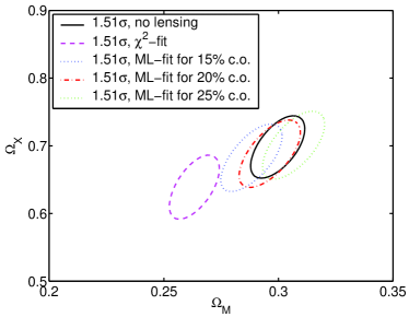
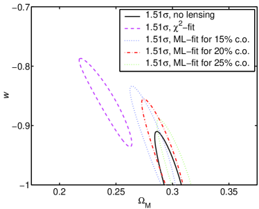
confidence region when no lensing effects have been considered while the dashed curve is the $\chi^{2}$-fit of for a dark matter model of 20 % compact objects (cf. Fig. 1). The dash-dotted curves show the ml-fits using the correct pdf, which is reducing the bias significantly as compared with the simple $\chi^{2}$-fit. The dotted curves show the result of an ml-fit when fractions of 15 % and 25 % compact objects are assumed when the true value is 20 %. These contours represent the expected systematic bias when under- or overestimating the fraction of dark matter in compact objects with 5 %. The results are a big improvement over the $\chi^{2}$-analysis. Thus, it should be possible to reduce the bias due to lensing in a fairly effective way, even with the simple approach used in this note.

8 Summary and discussion

Neglecting gravitational lensing effects may cause systematic errors when determining cosmological parameters using the distance-redshift relation for Type Ia SNe. E.g., if the universe contains a large fraction of compact objects, the matter density $\Omega_{\rm M}$ can be severely underestimated or a cosmological constant may be wrongly excluded if one assumes a Gaussian distribution of magnitudes. Using an approximately correct pdf for the SNe magnitudes, this bias can be reduced significantly.

In this note, we show that lensing effects can be parametrized in a simple way by the fraction of compact objects, $f_{\rm p}$, and the redshift. In general, lensing effects are bigger for larger values of $f_{\rm p}$ and higher redshifts. If $f_{\rm p}$ can be determined with $<5$ % accuracy, the bias in the cosmological parameter determination can be effectively reduced as compared to the case where the magnitudes are assumed to be Gaussian distributed. For future surveys, e.g., by the proposed snap satellite aiming at doing precision cosmology with Type Ia SNe, this reduction is essential to get systematic errors comparable to the statistical errors.

For the simple analysis performed in this note, we have first determined $f_{\rm p}$ to be able to choose the correct pdf for the subsequent parameter determination. Another possibility is to make a simultaneous fit of, e.g., $(f_{\rm p},\Omega_{\rm M},\Omega_{X},\cal M)$ which will be the aim of some forthcoming work.

References

- (1) Aldering, G., Supernova Factory Webpage, http://snfactory.lbl.gov
- Bergström et al. (2000) Bergström, L., Goliath, M., Goobar, A., & Mörtsell, E., 2000, A&A, 358, 13
- Browne (2000) Browne, I. W. A. 2000, in ASP Conf. Ser., Gravitational Lensing: Recent Progress and Future Goals, ed. T. G. Brainerd & C. S. Kochanek (San Francisco: ASP).
- Chiba & Yoshii (1999) Chiba, M., &, Yoshii, Y., 1999, ApJ, 1999, 510, 42
- Falco et al. (1998) Falco, E. E., Kochanek, C. S., & Munoz, J. A., 1998, ApJ, 494, 47
- Goliath & Mörtsell (2000) Goliath, M., & Mörtsell, E., 2000, Physics Letters B, 486, 249
- Goliath et al. (2001) Goliath, M., Amanullah, R., Astier, P., Goobar, A., & Pain, R., 2001, A&A 380, 6
- Goobar et al. (2002a) Goobar, A., Mortsell, E., Amanullah, R., Goliath, M., Bergström, L., & Dahlen, T., 2002, accepted for publication in A&A, astro-ph/0206409
- Goobar et al. (2002b) Goobar, A., Mortsell, E., Amanullah, R., & Nugent, P., 2002, accepted for publication in A&A, astro-ph/0207139
- Hennawi et al. (2001) Hennawi, J. F., Narayanan, V. K., Spergel, D. N., et al., 2001, AAS, 199, 1608
- Holz & Wald (1998) Holz, D. E., & Wald, R. M.,1998, Phys. Rev. D 58, 063501
- Keeton (2002) Keeton, C. R., 2002, accepted for publication in ApJL
- Kochaneck (1996) Kochanek, C. S., 1996, ApJ, 466, 638
- Koopmans & Fassnacht (1999) Koopmans, L. V. E., & Fassnacht, C. D. 1999, ApJ, 527, 513
- Metcalf & Silk (1999) Metcalf, R. B., & Silk, J., 1999, ApJ, 519, L1
- Mörtsell et al. (2001a) Mörtsell, E., Goobar, A., & Bergström, L., 2001, ApJ, 559, 53
- Mörtsell et al. (2001b) Mörtsell, E., Gunnarsson, C., & Goobar, A., 2001, ApJ, 561, 106
- Navarro et al. (1997) Navarro, J. F., Frenk, C. S., & White, S. D. M., 1997, ApJ 490, 493
- Seljak & Holz (1999) Seljak, U., & Holz, D., 1999, A&A, 351, 10
-
Perlmutter et al. (2000)
snap Science Proposal, available at
http://snap.lbl.gov - van Waerbeke et al. (2001) Van Waerbeke, L., Mellier, Y., Radovich, M., et al, 2001, A&A, 374, 757
- Wambsganss et al. (1997) Wambsganss, J., Cen, R., Xu, G., & Ostriker, J. P., 1997, ApJ, 475, L81