Spectroscopic Target Selection for the Sloan Digital Sky Survey:
The Luminous Red Galaxy Sample

Abstract

We describe the target selection and resulting properties of a spectroscopic sample of luminous, red galaxies (LRG) from the imaging data of the Sloan Digital Sky Survey (SDSS). These galaxies are selected on the basis of color and magnitude to yield a sample of luminous, intrinsically red galaxies that extends fainter and further than the main flux-limited portion of the SDSS galaxy spectroscopic sample. The sample is designed to impose a passively-evolving luminosity and rest-frame color cut to a redshift of 0.38. Additional, yet more luminous, red galaxies are included to a redshift of $\sim\!0.5$. Approximately 12 of these galaxies per square degree are targeted for spectroscopy, so the sample will number over 100,000 with the full survey. SDSS commissioning data indicate that the algorithm efficiently selects luminous ($M_{g^{*}}\approx-21.4$), red galaxies, that the spectroscopic success rate is very high, and that the resulting set of galaxies is approximately volume-limited out to $z=0.38$. When the SDSS is complete, the LRG spectroscopic sample will fill over $1h^{-3}{\rm\,Gpc^{3}}$ with an approximately homogeneous population of galaxies and will therefore be well suited to studies of large-scale structure and clusters out to $z=0.5$.

1 Introduction

The Sloan Digital Sky Survey (SDSS; York et al., 2000) combines a 5-band CCD imaging survey of the Northern Galactic Cap with an extensive and diverse multi-fiber spectroscopic follow-up program. The centerpiece of the spectroscopic survey is a sample of 1 million galaxies. This sample consists of two parts. The dominant portion, with about 88% of the fiber allocation, is a flux-limited sample (hereafter called MAIN) that will reach to approximately $r\sim 17.7$ (Strauss et al., 2001). This sample has a median redshift of 0.10 and few galaxies beyond $z=0.25$.

The other 12% of the galaxy spectroscopic sample is devoted to galaxies that are fainter than the MAIN galaxy flux cut but expected, based on the observed colors, to be intrinsically red and at higher redshift. The strong 4000Å break of early-type galaxies allows the SDSS to acquire redshifts for these fainter galaxies in the same amount of observing time despite a lower signal-to-noise ratio. At the outset, the goal of this luminous, red galaxy (LRG) survey was to produce a volume-limited sample of intrinsically luminous ($\gtrsim\!3L^{*}$), intrinsically red galaxies out to $z=0.5$. The term “volume-limited” means that the same population of galaxies would be traced across redshift. In principle, evolution and merging make this a poorly-defined concept. However, luminous, red galaxies (e.g. giant ellipticals) are observed to be evolving slowly (Oke & Sandage, 1968; Schild & Oke, 1971; Gunn & Oke, 1975; Rakos & Schombert, 1995; Kauffmann et al., 1996; Lubin, 1996; Oke et al., 1996; Ellis et al., 1997; Aragón-Salamanca et al., 1998; Collins & Mann, 1998; Stanford et al., 1998; van Dokkum et al., 1998; Burke et al., 2000), so we tune our selection to remove the passive evolution of an old stellar population. Other modes of evolution are left in the sample to be discovered.

A volume-limited sample of luminous, red galaxies is an efficient tool for a number of important science goals. First, because the brightest galaxies in galaxy clusters tend to be very luminous and red (Sandage, 1972; Hoessel et al., 1980; Schneider et al., 1983; Postman & Lauer, 1995), the LRG sample will include many luminous cluster galaxies and therefore will give spectroscopic redshifts for clusters selected from the SDSS imaging survey (e.g., Annis et al., 1999; Nichol et al., 2000; Goto et al., 2001; Kim et al., 2001). Second, the sample will probe over $1h^{-3}{\rm\,Gpc^{3}}$ with sufficient number density to yield an immense volume for the study of large-scale structure. Finally, the sample should permit studies of the evolution of giant elliptical galaxies from $z=0$ to $z=0.5$. The evolution of these systems is an important, if controversial, probe of hierarchical galaxy formation (Kauffmann, 1996; Aragón-Salamanca et al., 1998; Collins & Mann, 1998).

The purpose of this paper is to describe the selection algorithm used to select the LRG sample and to assess how the resulting sample approaches the design goals. We leave most details of the SDSS hardware and data reduction to other technical papers. York et al. (2000) provides an overview of the survey. The imaging data taken with the photometric camera (Gunn et al., 1998) through 5 filters (Fukugita et al., 1996) is reduced with the software pipeline photo (Lupton et al., 2001a, b). The photometric calibration is summarized in Stoughton et al. (2001). The target selection occurs within a software package known as target using the algorithm described in this paper. The targets are then distributed onto an adaptive mesh of plates (Blanton et al., 2001). Spectra are obtained by a pair of fiber-fed double spectrographs (Uomoto et al., 2001; Castander et al., 2001) and reduced by the spectro software pipeline (Frieman et al., 2001; Schlegel et al., 2001a). Further documentation of the survey can be found in the description of the Early Data Release (Stoughton et al., 2001).

The paper is arranged as follows. In §2, we describe the color-space context in which LRG selection occurs and then specify the cuts used to select the sample. The minor differences between the current algorithm and the algorithms used in the commissioning data are listed in Appendix A. We assess the photometric and spectroscopic performance of the sample in §3. In appendix B, we specify the models used to generate $K$ and evolutionary corrections for the data. We give advice and caveats about using the sample in §4 and conclude in §5.

We need to alert the reader to the fact that there are two different usages of the term “LRG sample” in this paper. On the one hand, the question facing LRG target selection is how to choose the spectroscopic targets fainter than the MAIN sample flux limit. Our assessment of sample efficiency, fiber quotas, and spectroscopic performance deals only with these targets. On the other hand, because LRGs are among the most luminous galaxies, it is clear that at $z\lesssim 0.3$ a volume-limited sample of LRGs will include some galaxies that are bright enough to be in the MAIN sample. Hence, assessments of the properties of the sample across redshift must include the LRGs from the MAIN sample. The choice of sample—LRGs with and without MAIN sample contributions—should be clear from context.

We have adopted a cosmology of $\Omega_{m}=0.33$ and $\Lambda=0.67$ for the calculation of distance moduli and comoving volumes. All absolute magnitudes and comoving volumes are quoted assuming $H_{0}=100{\rm\ km\ s^{-1}\ Mpc^{-1}}$.

2 Target Selection

2.1 Photometric Redshifts and LRGs

Galaxies vary significantly in their luminosities and spectral energy distributions (SEDs). Fortunately, their SEDs are sufficiently regular that one can attempt to infer their redshift from their colors (Baum, 1962; Koo, 1985; Loh & Spillar, 1986; Connolly et al., 1995). Were these photometric redshifts completely accurate, one could apply luminosity and intrinsic color cuts, and hence select the LRG sample, with fidelity. However, the fact that the redshifts estimated from photometry have errors complicates the isolation of the luminous, intrinsically red galaxies.

Figure 1: $u-g$ versus $g-r$ color for 6 non-evolving SEDs from Fukugita et al. (1995) and Kennicutt (1992) as a progression of redshifts. Redshift $z=0$ is at the end near the label, each solid dot represents an increment of 0.1 in redshift, and the last dots are $z=0.6$. The loci are reasonably separated in color-color space, indicating the possibility of accurate photometric redshifts.

Figure 2: As Figure 1, but for $g-r$ versus $r-i$. Here, the redshift loci for different SEDs lie on top of one another, indicating a photometric redshift degeneracy.

The errors in the photometric redshifts depend in detail upon the bandpasses and sensitivity of the SDSS. For an early-type galaxy, the 4000Å break provides a sharp feature in the SED from which we can infer the redshift. For $z<0.38$, this feature lies within the SDSS $g$ band. If all galaxies had the same SED, then the $g-r$ color would be an excellent redshift indicator. However, since galaxies actually show a range of 4000Å break strengths, $g-r$ actually measures only a degenerate combination of the position of the break (i.e. the redshift of the galaxy) and the strength of the break. One can break this degeneracy with the $u-g$ color, as shown in Figure 1. With these two colors, one could infer both the redshift and 4000Å break strength of the galaxy, which would allow selection of luminous, red galaxies.

Unfortunately, the galaxies of interest ($r\sim 19$) have $u\sim 22$, which is close to the SDSS detection limit so that the measured $u-g$ color of these objects is quite noisy. One must therefore turn to the $r-i$ color, which is well-measured. In principle, this second color would allow us to measure both redshift and SED type. However, as shown in Figure 2, galaxy SEDs suffer from an accidental degeneracy in the SDSS bands at $z<0.4$, such that early-type SEDs of lower redshift have the same $g-r$ and $r-i$ color as later-type SEDs of a higher redshift. In other words, galaxies of varying redshifts (less than 0.4) and SED form a nearly 1-dimensional locus in $g-r-i$ space; we cannot infer two quantities from the single position along this locus. As we will see, the bivariate luminosity-color distribution of galaxies does allow us to bypass this problem.

At $z>0.38$, the situation improves as the 4000Å break enters the $r$ band. The sensitivity of SDSS in $g$ is sufficient at $r\sim 19.5$ to yield a well-measured $g-r$ color, and one can combine this with $r-i$ to constrain the redshift independently of the SED of the galaxy. This can be seen in Figure 2 from the fact that the curves for the different SEDs do not overlap at $z>0.4$.

Because of this transition at $z\approx 0.4$, we are driven to use different selection cuts at $z\lesssim 0.4$ and $z\gtrsim 0.4$. At $z\lesssim 0.4$, we must extract LRGs out of the galaxy locus by relying on the bivariate galaxy luminosity and rest-frame color distribution to discriminate against bluer or less luminous galaxies. Similar selections have been performed by Warren et al. (1993), Gladders & Yee (2000), and Wilson et al. (2001). At $z\gtrsim 0.4$, it is easy to isolate the LRGs, although we will find that the finite spectroscopic integration time keeps us from fully extending to the desired luminosity cut.

2.2 SDSS Photometry

Consistency tests within the SDSS data indicate that the relative photometry of the survey is very good; however, the bandpasses of the filters are measured to be slightly different than designed (Fukugita et al., 1996; Fan et al., 2001; Stoughton et al., 2001), and the zero-point of the magnitude systems, which were intended to satisfy the ${\rm AB}_{95}$ convention, are still provisional. Hence, instead of referring to the magnitudes as $u$, $g$, $r$, $i$, and $z$, we refer to the current photometric solutions, as codified in the Early Data Release (Stoughton et al., 2001), as $u^{*}$, $g^{*}$, $r^{*}$, $i^{*}$, and $z^{*}$. This is a minor problem as regards the selection of LRGs, since the final calibration will only change the zeropoints of the magnitude system and hence move the selection cuts in easily calculable ways. However, at the time of this writing, the uncertainties over the bandpass shape and zeropoints create difficulties regarding the interpretation of the LRG spectroscopy. Because the sample spans a range of redshift, one must model the time-evolving SED of the galaxies in order to make corrections for the redshifting of the bandpasses and the evolution of the stellar populations. Those models do not produce colors that match our photometry, presumably in part because of some remaining problems in our knowledge of the filter shapes and zeropoints. The models and the corrections we apply are described in Appendix B.

2.3 Selection Cuts

As described above, we use different techniques above and below $z\approx 0.4$. The low-redshift cut, which accounts for 80-85% of the targets, will be called Cut I; the high-redshift cut will be called Cut II. As a matter of context, we note that the MAIN sample flux limit is $r^{*}\sim 17.7$, whereas the commissioning spectroscopic data show that a 45-minute exposure with the SDSS 2.5m telescope can acquire reliable redshifts on objects with strong 4000Å breaks as faint as $r^{*}\sim 19.5$. Hence, the LRG cuts are optimized to work in this range of magnitudes.

For both cuts, we rely on Petrosian (1976) magnitudes in the $r$ band to set our flux and surface brightness cuts. These magnitudes are calculated exactly as for the MAIN galaxy sample (Strauss et al., 2001), avoiding any discontinuity in the transition from the MAIN to LRG samples. The $r^{*}$ surface brightness is calculated using the radius inside which half the Petrosian flux is found, i.e.,

$$\mu_{r^{*},\rm Petro}=r^{*}_{\rm Petro}+2.5\log_{10}(2\pi R_{50}^{2}).$$ (1)

Again, this choice matches that of MAIN galaxy target selection.

For colors, we use the model magnitudes from photo. The best-fit exponential or de Vaucouleurs model, allowing for arbitrary scale length and axial ratio and convolving with the local point spread function, is found for each object in the $r$ band. That model is then used to extract the flux in the other bands. Since all bands are measured with the same effective aperture, the colors are unbiased in the absence of color gradients; the resulting colors have higher signal-to-noise ratio than a simple aperture color. All colors in LRG selection refer to differences of model magnitudes. Further details of model magnitudes can be found in Lupton et al. (2001b). Finally, the separation of stars from galaxies is done by differencing the $r^{*}$ model magnitude from the $r^{*}$ PSF magnitude, as described in Lupton et al. (2001b). This is the same method as for MAIN galaxy target selection, but we will use a different value for the threshold parameter.

All magnitudes and colors have been corrected for Galactic extinction using the Schlegel et al. (1998) map and assuming $R_{V}=3.1$.

Galaxy colors in the $g^{*}-r^{*}$ vs. $r^{*}-i^{*}$ plane display a narrow linear locus due to the degeneracy of early- to mid-type galaxies at $z<0.4$. We therefore adopt a rotated coordinate system in color-space so that we can measure position along and across that locus. The distance perpendicular to the locus is simply

$$c_{\perp}=(r^{*}-i^{*})-(g^{*}-r^{*})/4.0-0.18.$$ (2)

The intercept is chosen from the data so that $c_{\perp}=0$ marks the center of the observed locus.

For galaxies that lie in the locus, we wish to estimate where they fall along the locus. One could use the orthogonal complement of equation (2), but if we assume that galaxies fall along the line $c_{\perp}=0$, we are free to choose the linear combination of colors that minimizes the error in the estimator. In other words, because the error of $g^{*}-r^{*}$ is different from that of $r^{*}-i^{*}$, one may get a more accurate estimate of the position of the galaxy along the locus by weighing one color more than the other. Given the average errors on these three magnitudes for galaxies in the given flux and color range, we adopt

$$c_{\parallel}=C(g^{*}-r^{*})+(1-C)4.0[(r^{*}-i^{*})-0.18].$$ (3)

The definition is chosen so that an object with $c_{\perp}=0$ has $c_{\parallel}=g^{*}-r^{*}$. We use $C=0.7$. In principle, one could have chosen $C$ on an object-by-object basis so as to minimize the error on $c_{\parallel}$ given the quoted errors on the colors. However, this would have reduced the formal errors only slightly at the expense of requiring the formulae to depend sensitively on the quoted errors.

In fact, the error on $c_{\parallel}$ is insensitive to the choice of $C$, but our choice does help in a different fashion. Although the early-type color-color locus makes a sharp turn at $z\approx 0.4$, the galaxies do not move out of the $z<0.4$ locus immediately, simply because of the non-zero thickness of that locus. By choosing $C=0.7$ as opposed to 16/17 (which would have established a strictly orthogonal system), galaxies at $z>0.4$ still have $c_{\parallel}$ grow with redshift. This procedure makes Cut I effective to slightly higher redshifts than one would have guessed a priori.

Objects that are flagged by photo as BRIGHT or SATURated in $g^{*}$, $r^{*}$, or $i^{*}$ are excluded. Objects must be detected as BINNED1, BINNED2, or BINNED4 in both $r^{*}$ and $i^{*}$, but not necessarily in $g^{*}$. These flags are explained in Stoughton et al. (2001). The BINNED flags indicate that the object is detected in the particular band, where detected means that one or more (original or $2\times 2$ or $4\times 4$ re-binned) pixels is more than 5-$\sigma$ above the sky level. Since the faintest LRG candidates are quite faint in $g^{*}$, we do not wish to require such a detection in that band; however, 99% of the targets are in fact so detected in $g^{*}$. As with all SDSS target selection, objects are considered after deblending, with each fragment judged separately.

LRG target selection in the commissioning data (Stoughton et al., 2001) used slightly different cuts than those described below. The differences are listed in Appendix A.

2.3.1 Cut I ($z\lesssim 0.4$)

Figure 3: Petrosian $r^{*}$ apparent magnitude versus observed color $c_{\parallel}$ for a set of galaxies from SDSS. The solid lines show the selection region for Cut I LRGs. The dashed lines show three loci predicted by a stellar population synthesis model for galaxies as a function of redshift. The top line is for a passively-evolving old population (appendix B); the lower two lines mix in progressively more late-time star formation. Of course, changing the absolute magnitude of a galaxy will shift the lines horizontally; the displayed lines have $z=0$ $r^{*}$ absolute magnitudes of $-22.2$, $-21.7$, and $-21.7$, top to bottom. We use the fact that the old population has a nearly linear magnitude-color relation in our selection cut. The data are taken from SDSS imaging runs 752 and 756 with $185^{\circ}<\alpha<235^{\circ}$ and $|\delta|<1.25^{\circ}$, excluding a few fields from run 752 with $r^{*}$ seeing FWHM worse than $2^{\prime\prime}$ (Stoughton et al., 2001).

Figure 4: The $g^{*}-r^{*}$ versus $r^{*}-i^{*}$ color-color diagram for galaxies with $18.5<r^{*}<19.5$ from SDSS. The red solid lines show the selection region for Cut I LRGs. The three lines overlaid with an arrow indicates that the location of the line cutting across the galaxy locus is a function of $r^{*}$ apparent magnitude; fainter galaxies must be redder to pass the cut. The displayed lines correspond to $r^{*}=17.5$, 18.0, and 18.5, left to right. The blue short-dashed lines show the (magnitude-independent) selection region for Cut II LRGs. The long-dashed line shows the locus of a passively-evolving old population as a function of redshift (appendix B); the bend in the locus occurs at $z\approx 0.40$. The galaxy sample is the same as in Figure 3.

Figure 5: Petrosian $r^{*}$ apparent magnitude versus Petrosian $r^{*}$ half-light surface brightness $\mu_{r^{*},\rm Petro}$ for 1700 galaxies that would otherwise pass either of the LRG cuts. Only the flux cut (eq. [5]) and surface brightness cuts (eqs. [7] and [12]) have been omitted. One sees that the surface brightness cut, indicated by the dashed line, eliminates only a small fraction of potential targets. A number of junk objects, e.g. scattered light, occur at $\mu_{r^{*},\rm Petro}>26$. The data from which these objects were selected is as in Figure 3.

Figure 6: Petrosian $r^{*}$ apparent magnitude versus $r^{*}_{\rm psf}-r^{*}_{\rm model}$, the quantity used for star-galaxy separation. (top panel) All objects that pass Cut I excluding the star-galaxy separation cut. Fainter magnitudes have fewer stars because the color cuts have moved away from the stellar locus. (bottom panel) Same, but for Cut II. One sees that the ratio of stars to galaxies is less favorable for Cut II, hence the more restrictive threshold of 0.5 rather than 0.3. Of the few stars discovered spectroscopically in the sample above the threshold, many fall well above the cut. Undeblended close pairs of stars as well as faint stars with superposed diffraction spikes from bright companions can boost $r^{*}_{\rm model}$ significantly brightward of $r^{*}_{\rm psf}$. The region of the data is as in Figure 3.

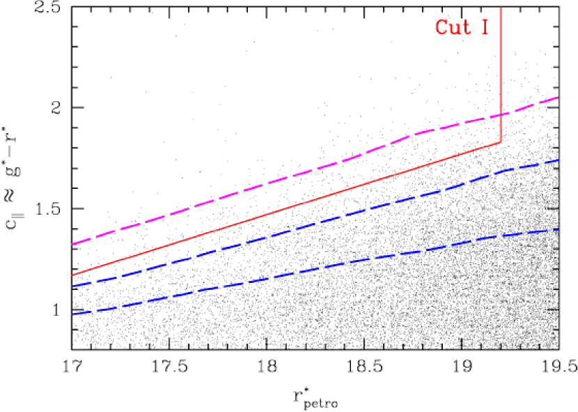
Cut I uses $c_{\parallel}$ as a redshift indicator and uses a sliding flux cut so as to approach a constant passively-evolving luminosity cut. We consider the locus of $r^{*}$ vs. $c_{\parallel}$ for an old single-age stellar population. For all models considered, this locus is nearly linear across the redshift range of interest, as shown in Figure 3. Therefore, we select objects that satisfy

$$r^{*}_{\rm Petro} < 13.1+c_{\parallel}/0.3,$$ (4)

$$r^{*}_{\rm Petro} < 19.2,$$ (5)

$$|c_{\perp}| < 0.2,$$ (6)

$$\mu_{r^{*},\rm Petro} < 24.2{\rm\ mag\ arcsec^{-2}},$$ (7)

$$r^{*}_{\rm psf}-r^{*}_{\rm model} > 0.3.$$ (8)

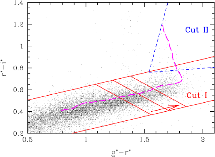
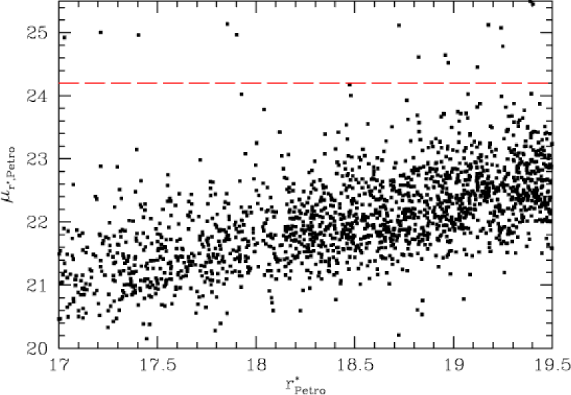
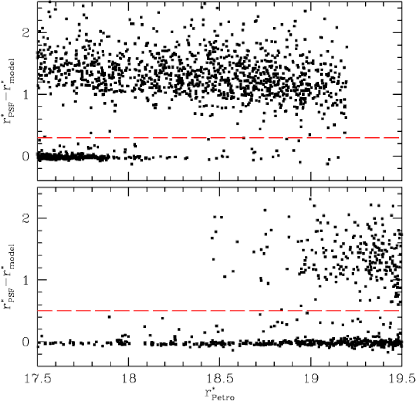
Equation (4) is the most important, because it is primarily responsible for setting the luminosity threshold as a function of redshift. Equation (5) imposes a flux cut chosen in large part to ensure good spectroscopic performance. The $c_{\perp}$ cut restricts attention to the $z<0.4$ galaxy locus (see Figure 4). The $\mu_{r^{*},\rm Petro}$ cut removes very low surface brightness objects that are often reduction errors of various sorts, e.g. deblended diffraction spikes or scattered light (Strauss et al., 2001). This cut is important because such objects can have strange colors. As shown in Figure 5, the surface brightness threshold is safely fainter than most LRG candidates. The $r^{*}_{\rm psf}-r^{*}_{\rm model}$ cut is our star-galaxy separator. Again, as shown in Figure 6a, most Cut I LRGs are safely away from this cut.

As additional quality assurance cuts, we exclude objects that have $g^{*}-r^{*}>2.5$, $r^{*}-i^{*}>1.5$, or estimated errors on the model magnitudes exceeding 0.2, 0.1, or 0.1 mag in $g^{*}$, $r^{*}$, and $i^{*}$, respectively. Very few objects fail any of these cuts without also failing the $\mu_{r^{*},\rm Petro}$ cut.

The number of objects selected is extremely sensitive to the color-magnitude cut in equation (4). A shift of 0.01 in $c_{\parallel}$ or 0.03 in $r^{*}_{\rm Petro}$ makes a 10% change to the number of galaxies selected. We will discuss this further in § 4.2.

As we discussed above, $c_{\parallel}$ alone is not sufficient to predict the redshift of a galaxy. Intrinsically bluer galaxies at higher redshifts or intrinsically redder galaxies at lower redshifts can produce the same colors (Fig. 2). However, Cut I turns out to be extremely effective at selecting LRGs. The reason is the shape of the bivariate luminosity-color function, not the success of photometric redshifts. Intrinsically redder galaxies at lower redshift—and hence lower luminosity at a given flux—would satisfy the cut, but there are few luminous galaxies redder than the old stellar populations of giant elliptical and cD galaxies. Conversely, intrinsically bluer galaxies at higher redshift and higher luminosity would pass the cut, but such super-luminous galaxies are extremely rare. Hence, as will be shown later, most of the galaxies that pass the cut turn out to have redshifts that place their intrinsic colors and luminosities in the ranges appropriate for old stellar systems well above $L^{*}$.

Objects that satisfy both the LRG cut and the MAIN cut are flagged as both by the target pipeline. However, the linear color-magnitude cut (eq. [4]) is not a good approximation to the locus of an early-type galaxy at lower redshifts. At $z<0.15$, Cut I is too permissive, allowing lower luminosity sources to enter the LRG sample. Hence, to extract LRGs from the MAIN sample at $z<0.15$, one must make additional post-spectroscopic cuts. These are described in § 4.1.

2.3.2 Cut II ($z\gtrsim 0.4$)

Cut II is used to select LRGs at $z>0.4$ by identifying galaxies that have left the low-redshift locus in the $g^{*}-r^{*}$ vs. $r^{*}-i^{*}$ plane. At these redshifts, we can distinguish 4000Å break strength from redshift, so we can isolate intrinsically red galaxies. The difficulty is avoiding interlopers, either from $z\lesssim 0.4$ galaxies that scatter up in color from the low-redshift locus or from late-type stars, which are far more numerous.

We adopt $r^{*}_{\rm Petro}=19.5$ as our flux limit because fainter objects would not reliably yield sufficient signal-to-noise ratio in the spectra. Unfortunately, the luminosity threshold in Cut I would predict $r^{*}_{\rm Petro}>19.5$ at the redshifts of interest in Cut II. Therefore, Cut II is simply a flux-limited sample with no attempt to produce a fixed luminosity cut across the (narrow) range of redshift probed.

The selection imposed is

$$r^{*}_{\rm Petro} < 19.5,$$ (9)

$$c_{\perp} > 0.45-(g^{*}-r^{*})/6,$$ (10)

$$g^{*}-r^{*} > 1.30+0.25(r^{*}-i^{*}).$$ (11)

$$\mu_{r^{*},\rm Petro} < 24.2,$$ (12)

$$r^{*}_{\rm psf}-r^{*}_{\rm model} > 0.5,$$ (13)

Equation (10) separates the high-redshift region from the low-redshift galaxy locus. It is tilted in $c_{\perp}$ to guard against the larger areal number density of prospective interlopers at lower $g^{*}-r^{*}$. Equation (11) isolates intrinsically red galaxies and separates the selected region from the bulk of the late-type stellar locus. These cuts are displayed in Figure 4. Equation (12) places the same surface brightness cut as in cut I. As before, this is primarily a quality assurance cut. Finally, equation (13) implements the star-galaxy separation; because of the larger ratio of stellar objects to galaxies in the color-magnitude region, we adopt a stronger cut than in Cut I (see Figure 6b). We again exclude objects with $g^{*}-r^{*}>2.5$, $r^{*}-i^{*}>1.5$, or errors on the model magnitudes exceeding 0.2, 0.1, or 0.1 mag in $g^{*}$, $r^{*}$, and $i^{*}$, respectively. Note that the $r^{*}-i^{*}$ cut here does exclude a few very late-type stars, whereas early-type galaxies are not predicted to get this red, even for $z>0.6$.

The threshold of $c_{\perp}$ needed to keep away from the low-redshift locus restricts Cut II to $z\gtrsim 0.43$. Fortunately, Cut I includes plenty of galaxies in the range $0.38<z<0.44$ because of the definition of $c_{\parallel}$.

3 Performance in Commissioning Data

Many thousand spectra of LRGs have been acquired by the SDSS thus far. The SDSS uses a pair of fiber-fed double spectrographs to cover the wavelength range from 3800Å to 9200Å with a resolution of $\sim\!1800$ ($\sim\!150\rm\ km\ s^{-1}$ FWHM). The diameter of the fibers are $3^{\prime\prime}$. These spectra allow a detailed study of the properties of the objects selected by the LRG cut.

Figure 7: Spectra of 5 LRG, with the wavelengths shifted to the rest-frame. The top four spectra are taken from plate 383 observed on MJD 51818. This plate exceeded the survey minimum signal-to-noise ratio by about 20%, which is fairly typical. The top 3 spectra (fibers 247, 19, and 193) show a progression of redshift, while the 4th (fiber 199) is an unusual spectrum showing [O II] $\lambda 3727$ emission. The last spectrum is fiber 416 from plate 394 observed on MJD 51913. We obtained much more signal on this plate, about 2.5 times the survey minimum signal-to-noise ratio. This spectrum shows strong Balmer absorption characteristic of E+A galaxy spectra. The spectra have been slightly smoothed for presentation.

A sample of LRG spectra are displayed in Figure 7. The signal-to-noise ratio in the first four spectra are typical of the survey; the bottom spectrum is well above the usual survey quality. The first three spectra illustrate a progression of redshift, the fourth spectrum shows a mild emission line, and the last spectrum shows extra Balmer absorption characteristic of E+A galaxy spectra (Dressler & Gunn, 1983). The latter two phenomena occur only rarely in the sample.

For a careful determination of the redshift distribution and failure modes, we focus on a sample of 21 plates. These were picked to be in chunks 8, 9, 10, and 11 so that the final selection could be implemented exactly (see Appendix A for an explanation of how targets were selected in the commissioning data as well as a definition of the term “chunk”). 14 of these plates have duplicate observations of survey quality. Since the highest signal-to-noise ratio example of each plate was picked, the primary set of 21 tends to have signal-to-noise ratios significantly above the survey minimum. These plates have 972 objects selected by Cut I and 165 selected by Cut II (all fainter than the MAIN survey). We inspected all of these spectra by eye to validate the redshift assigned by the spectro pipeline. A few mistakes were fixed, and a few unknown cases were determined by eye. The result is a very complete and accurate redshift catalog.

For the measurement of quantities where large-scale structure is the dominant uncertainty, we use a larger sample of plates. This includes 8267 Cut I and 1284 Cut II LRG targets on 173 plates from Chunks 4-13. In cases where an object was observed multiple times, either because the plate was observed twice or because of quality-assurance fiber allocation, the highest signal-to-noise ratio spectrum was used (as measured by the median signal-to-noise ratio of the plate). Some figures use a randomly selected subsample of these plates, simply to reduce the density of points.

3.1 Redshifts and derived quantities

We begin by describing the results of the spectroscopy, focusing on the set of 21 verified plates. Of the 972 Cut I LRG targets on these plates, 7 were stars. The remainder had redshifts between 0.10 and 0.53, of which only 4 were at $z<0.2$. None of the spectra failed to yield a redshift when examined by eye, although data problems (e.g. large patches of missing data because of bad CCD columns) made a few cases difficult. Nearly all were early-type galaxy spectra, but some have emission lines in addition.

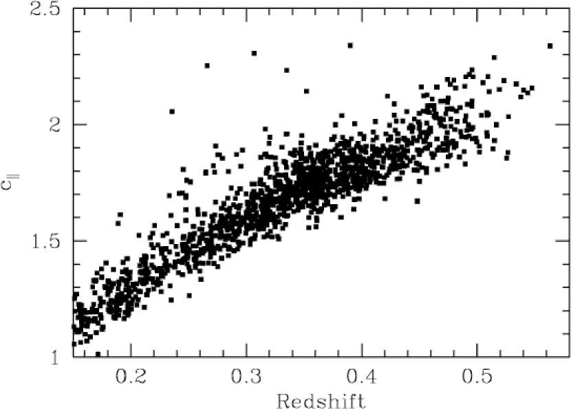
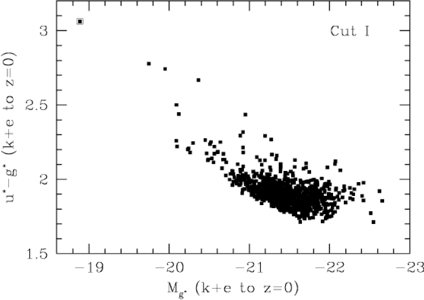
Figure 8 plots redshift versus $c_{\parallel}$ color. Clearly, most galaxies fall along a tight correlation. Excluding 4% of the points as outliers, the rms scatter in $c_{\parallel}$ from a linear fit is $\sim\!0.065$ mag at $z<0.35$ and $\sim\!0.08$ mag at $z>0.35$. The scatter in redshift is 0.02 at $z<0.35$ and 0.03 at $z>0.35$. A few percent of objects have redshifts that are low for an old stellar population of their color; turning this around, one would say that their rest-frame colors are redder than an old population given their redshift. The most extreme example of this is an edge-on disk galaxy at $z=0.108$, in which dust extinction is presumably strongly reddening the colors. Close binary pairs of galaxies are another form of outlier; the deblending algorithm (Lupton et al., 2001b) can occasionally deblend the different bands inconsistently (this behavior will be improved with future versions of the algorithm). If one is interested in a strict sample of luminous galaxies with old stellar populations, one should reject objects with rest-frame colors that are too red. Even if the color became too red because of an error in the photometry, the red claimed color means that the apparent magnitude cut is too permissive. The result is that nearly all these objects are far less luminous than one intended, as shown in the absolute magnitude versus rest-frame color plot in Figure 9. As described in Appendix B, we use the measured redshift and the observed $r^{*}_{\rm Petro}$ magnitude and $g^{*}-i^{*}$ color to construct the rest-frame, passively-evolved $g^{*}_{\rm Petro}$ absolute magnitude and $u^{*}-g^{*}$ color. In this sample, only 7 objects (including the edge-on disk mentioned above) have rest-frame $u^{*}-g^{*}>2.35$ and 41 more have $2.1<u^{*}-g^{*}<2.35$, as compared to a typical $u^{*}-g^{*}$ of around 1.9. No object is significantly too blue for its redshift. Conservatively, then, one would call the sample 95% efficient at selecting luminous, red galaxies.

Figure 8: Redshift versus $c_{\parallel}$ color for LRGs, including objects from the MAIN sample that pass an LRG cut (always Cut I) and have $z>0.15$.

Figure 9: Absolute magnitude versus rest-frame color for 965 Cut I LRGs from our sample of 21 verified plates. Both quantities have been $K$-corrected and passively-evolved to $z=0$ using the prescription in Appendix B. The sharp diagonal boundary in rest-frame $u^{*}-g^{*}$ versus $M_{g^{*}}$ is the result of the color-magnitude selection in equation (4). The edge-on disk galaxy at $z=0.108$ is marked (dot in open square) as an extreme example of how an object much redder than an old stellar population can enter the sample.

Figure 10: Absolute magnitude versus rest-frame color for 150 Cut II LRGs from our sample of 21 verified plates. Both quantities have been $K$-corrected and passively-evolved to $z=0$. Galaxies at $z<0.4$ have been marked as dots in open squares; the object at $z=0.08$ falls off the plot faintward and blueward. Note that the bounding region of the cut is not sloped as for Cut I (see Fig. 9).

Figure 11: Comparison of the absolute magnitude and rest-frame color distribution of MAIN galaxies (dots) and LRGs (crosses) from our sample of 21 verified plates. The quantities on both axes have been $K$-corrected and passively-evolved to $z=0$. Only MAIN galaxies with redshifts between 0.05 and 0.15 and LRGs at $z>0.2$ (including those from the MAIN sample) are shown. The dashed line shows the rough position of $M^{*}$ from the luminosity function of MAIN galaxies (Blanton et al., 2001). Additionally, the MAIN sample is approximately volume-limited to the right of the dashed line. One sees that the LRGs populate the luminous end of the red sequence. The offset in the color of the red sequence between the MAIN and LRG samples is presumably due to errors in the photometric zeropoints and/or errors in the broadband shapes of the stellar population synthesis models used to correct colors to zero redshift.

Of the 165 Cut II LRGs, 11 were stars. Four others had spectra with too little signal to find a secure redshift; it turns out that one of these was a deblended diffraction spike from a bright star. Of the objects with confirmed $z>0$ redshifts, one is a $z=0.08$ galaxy with a late-type star superposed and three others have $z<0.38$ and fall outside of the $M_{r^{*}}$ vs. $g^{*}-r^{*}$ region populated by Cut I galaxies. The remaining 146 have redshifts between 0.38 and 0.57; all but five have $z>0.42$. Combining the 11 stars with the four lower-redshift galaxies implies a success rate of finding luminous, red galaxies of about 90%.

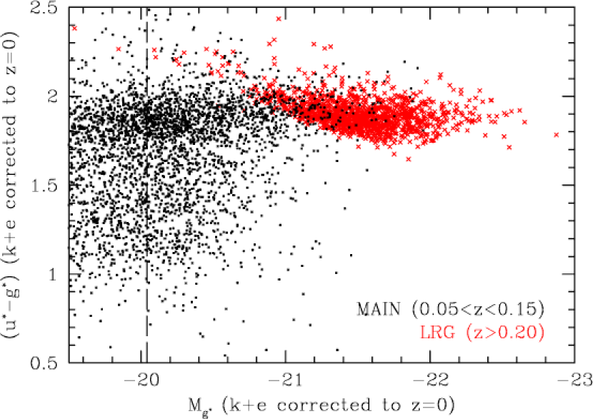
Figure 10 shows the distribution of absolute magnitudes and rest-frame colors for Cut II galaxies. Comparing this to the results for Cut I in Figure 9 reveals significant differences between the two samples. Cut II achieves a threshold in luminosity that is approximately independent of rest-frame color, whereas Cut I has a strong correlation between the two. In both cases, however, the selected galaxies do occupy the luminous, red tail of the galaxy distribution. This is shown in Figure 11, which overplots the LRG sample against a volume-limited sample of MAIN galaxies.

3.2 Photometric Properties

Figure 12: The comoving number density of LRGs as a function of redshift. The shaded regions from left to right indicate LRGs from the MAIN sample, Cut I (fainter than the MAIN flux limit), and Cut II contributions. The numbers indicate the number of galaxies in each bin.

Figure 13: Redshift versus $z=0$ absolute $g^{*}$ magnitude for 4500 LRGs. The abscissa has been remapped to show the enclosed comoving volume for a survey of $\pi$ steradians as a function of redshift. Dashed lines show increments of redshift. The ordinate has been passively-evolved and $K$-corrected to $z=0$. This means that a sample of constant comoving volume will have an even density of objects. LRGs from MAIN, Cut I, and Cut II are shown in black dots, red crosses, and blue squares, respectively. The apparent magnitude cuts are clearly visible as the diagonal transitions.

Figure 14: As Figure 13, but the ordinate has been replaced by a combination of absolute magnitude and rest-frame color (both $K+e$ corrected to $z=0$) that lies parallel to the LRG boundary line in Figure 9. This shows that the boundary of the selection is rather sharp and moves only slightly with redshift for $z<0.4$.

Figure 15: The effective radius of the best-fit de Vaucouleurs model in the $r$ band versus redshift for LRGs. While the model fit is done including the convolution of the point spread function, we only include objects with $r$ band seeing better than 1^′′.4 just to minimize any seeing effect. The dashed line shows the length corresponding to 1^′′. The median radius increases slightly with redshift; one possible cause of this might be the increasing luminosity threshold at $z>0.4$.

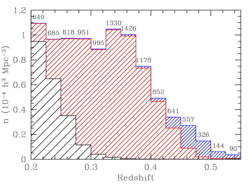
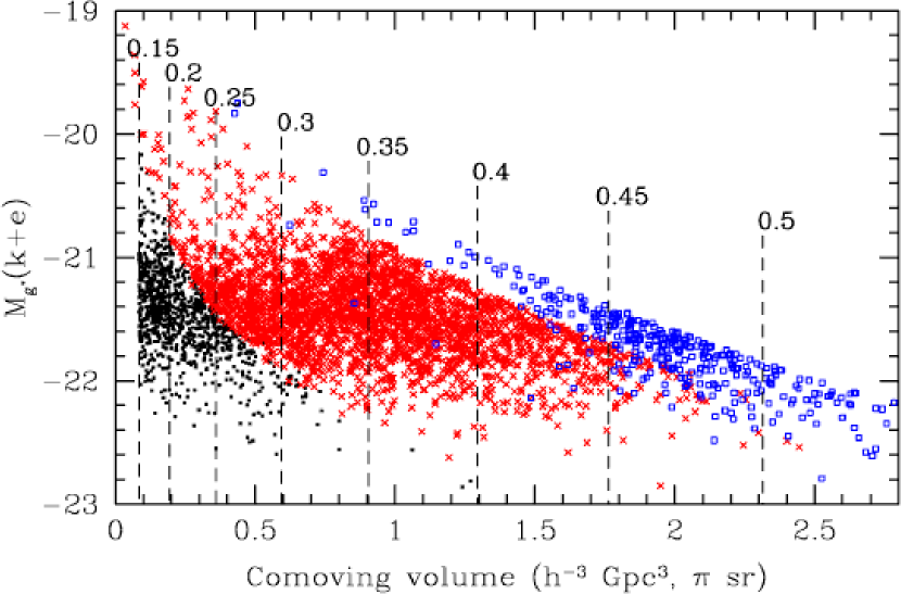
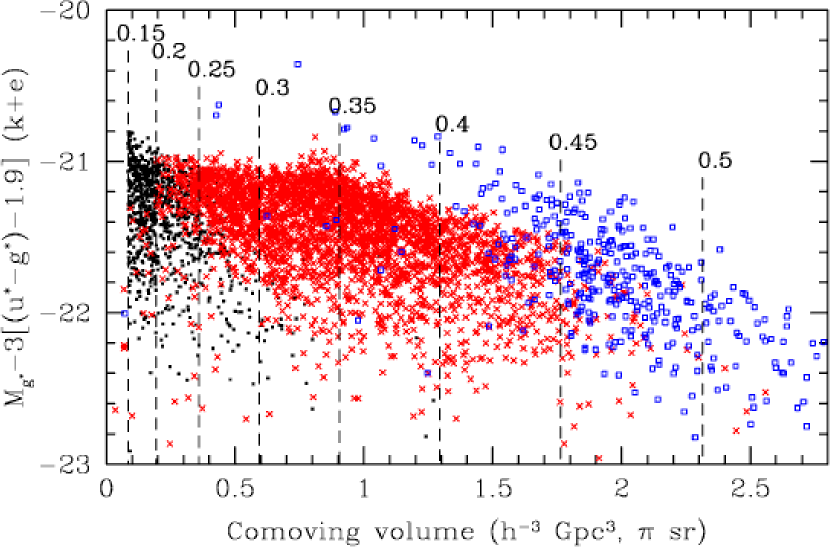
A design goal of the sample is to produce a nearly volume-limited set of luminous, red galaxies. This concept cannot be precisely realized in the context of a merging galaxy population, but we can offer a few results that are suggestive of a volume-limited sample. In particular, we study the comoving density and passively-evolved luminosity thresholds as functions of redshift and show that these are nearly constant for $z<0.4$.

Figure 12 shows the comoving number density of LRGs from 173 plates. The sample has a nearly constant density to $z\approx 0.4$, with dropping density beyond.

Figure 13 shows the distribution of redshift and absolute magnitude. The latter has been corrected for passive evolution of an old stellar population. The redshift axis has been warped so as to show the enclosed comoving volume; this means that a sample of constant comoving density would have a constant density of points. The lines of constant apparent magnitude are clearly seen as the transition between different types of points. The sample appears to have a fairly constant luminosity threshold to $z\approx 0.35$, at which point the flux limits of the cuts impose a floor. However, the blurred appearance of the luminosity cut is not caused by measurement errors but rather by the variation of the cut with rest-frame color, as shown in Figure 9.

We can correct for this correlation of luminosity and color by measuring the offset of the galaxies from the diagonal boundary in Figure 11. This is shown in Figure 14. Here we see that the boundary is fairly sharp. The boundary appears to be fairly constant for $0.2<z<0.4$. At larger redshifts, Cut I has a clear downturn, while Cut II seems to be lower in comoving density. The upturn near $z\approx 0.15$ is real and will be discussed in § 4.1.

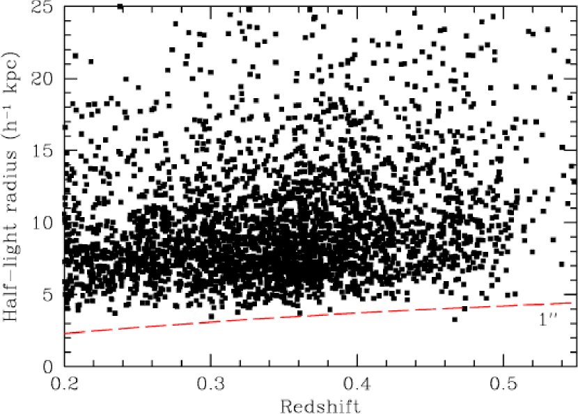
In addition to approximately constant luminosities, the LRGs also show constant physical size out to $z\approx 0.4$, as shown in Figure 15. The increase in size at $z>0.4$ is expected because those galaxies are more luminous on average. We have used the effective radius of the best-fit seeing-convolved de Vaucouleurs model to define the size.

In summary, the LRG sample appears to have approximately constant passively-evolved selection, physical size, and comoving number density out to $z\approx 0.4$. From this, we would say that the sample is approximately volume-limited, but we caution that small changes in the $K+e$ corrections or assumed cosmology might hide modest differences in the selected galaxies between low and high redshift. Evolution in color is particularly difficult to constrain within the uncertainties of the modeling. However, we do find that primary effects of changing the value of $\Omega_{m}$ is to shift all of the number densities and $z=0$ absolute magnitudes uniformly without introducing a large offset between redshifts of 0.2 and 0.4.

3.3 Spectral Quality and Repeatability

Figure 16: Redshift versus 3^′′ aperture (“fiber”) $r^{*}$ magnitude for LRGs on the 21 verified plates. The 4 objects for which no redshift was attained are shown as crosses on the right of the plot.

One can use the duplicate observations of the eye-inspected plates to quantify the spectral repeatability. Here we consider only duplicate observations with signal-to-noise ratio exceeding survey minima and only include objects that were spectroscopically confirmed as extragalactic. This gave 588 Cut I and 82 Cut II objects with duplicate observations. The average signal-to-noise ratio of these duplicates exceeds the minimum allowed (by definition) by 30%, which is typical of observations in good conditions.

Of the 588 Cut I duplicates, only five differed catastrophically ($>1000$ $\rm\ km\ s^{-1}$) in redshift according to automated software (Schlegel et al., 2001b). Three of these five could have their redshifts identified by eye; the other two suffered from large stretches of missing spectrum (this is usually due to bad CCD columns). Hence, to the eye, one has only two failures, both because of missing data. The rms velocity difference of the 583 cases that agreed was 73 $\rm\ km\ s^{-1}$although this drops to 61 $\rm\ km\ s^{-1}$ if one excludes nine outliers with velocity differences between 250 $\rm\ km\ s^{-1}$ and 500 $\rm\ km\ s^{-1}$. Note that the uncertainty in a single measurement would be $\sqrt{2}$ lower than this if the two measurements had equal errors; the correction here would be somewhat less because we are interested in the error of the lower quality measurement. One would reasonably say that the redshift error is around 50 $\rm\ km\ s^{-1}$ rms. Note that survey performance on the MAIN galaxy sample is considerably better than this because the targets are brighter (Strauss et al., 2001).

Of the 82 Cut II duplicates, one again finds five catastrophic errors ($>1000$ $\rm\ km\ s^{-1}$) from the automated software. Three were recovered by eye; two were too low in signal-to-noise ratio to securely state the redshift. The rms velocity difference of the remaining 77 was 150 $\rm\ km\ s^{-1}$, but this drops to 113 $\rm\ km\ s^{-1}$ if three outliers of more than 350 $\rm\ km\ s^{-1}$ are dropped. Obviously, errors of several hundred $\rm\ km\ s^{-1}$ are severe and indicate that the precise redshift is being based on a small number of noisy absorption lines while the crude redshift is constrained by the 4000Å break. Again, the above rms differences should be divided by a factor just shy of $\sqrt{2}$, so one could claim rms errors in Cut II of about 100 $\rm\ km\ s^{-1}$.

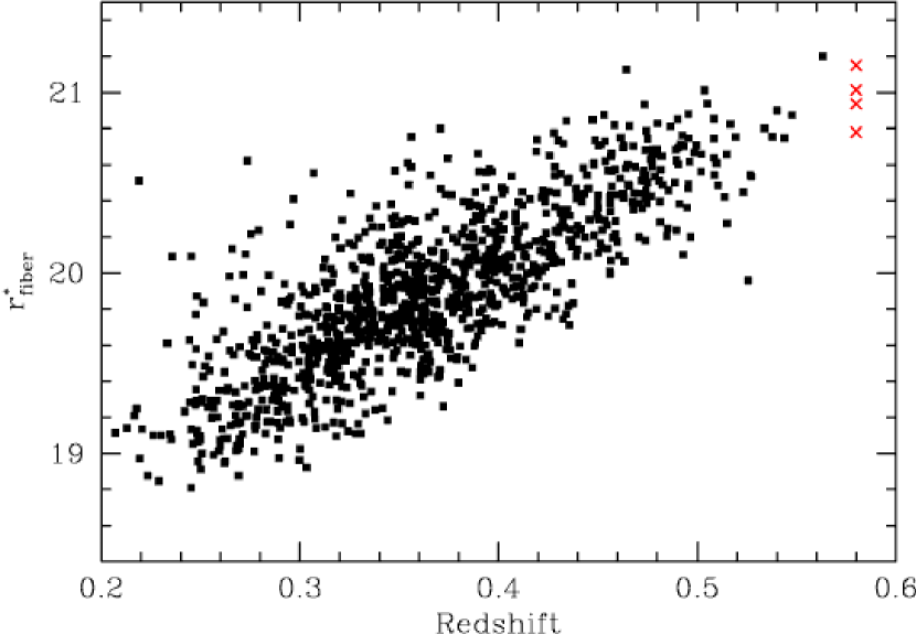
The LRGs are among the faintest objects targeted by the SDSS, and we expect that the faintest of the LRGs will have incompleteness due to inadequate signal-to-noise ratio in the spectra. Figure 16 shows the distribution of redshift versus 3^′′ diameter aperture magnitudes (3^′′ is the input diameter of the spectroscopic fiber). The four objects for which we fail to get a redshift fall at the faint end of the magnitude distribution.

4 Using the LRG Sample

The SDSS target pipeline sets two flags for the LRG sample. The GALAXY_RED flag is set if the object passes either Cut I or Cut II. The GALAXY_RED_II flag is set if the object passes Cut II but not Cut I. If an object is brighter than the MAIN sample flux cut, then neither flag is set if the object failed to enter the MAIN sample (for example, because of the MAIN sample surface brightness cut). In other words, LRG target selection never overrules MAIN target selection on brighter objects.

As will be described below, the LRG cuts do not preserve the luminosity threshold at $z<0.2$. Therefore, the simplest prescription for using the LRG sample is to select objects with the GALAXY_RED flag and redshifts $z>0.2$.

4.1 Extracting low-redshift LRGs from the MAIN sample

The LRG flags are set when a MAIN galaxy passes either of the LRG cuts. This may lead to the impression that such galaxies are physically similar to the LRGs at higher redshift. However, this is incorrect because the LRG selection cuts were not designed to track the color-magnitude locus of luminous, red galaxies to lower redshifts. Indeed, such a prescription would be essentially impossible as $z\rightarrow 0$ because the observed color would not change while the distance modulus would diverge and hence the absolute magnitude would become unbounded. The sense of the breakdown of the LRG cuts is that they become too permissive; the linear color-magnitude cut (eq. [4]) allows underluminous galaxies to enter the sample.

It is of course necessary to include the LRGs from MAIN at $z\lesssim 0.3$ because the more luminous LRGs are above the MAIN flux cut, as shown in Figures 12 and 13. In detail, the imposed color-magnitude cut generates a constant passively-evolving luminosity selection down to $z=0.2$. LRG-selected galaxies with $0.15<z<0.2$ could be used, but the luminosity cut will be fainter by about 0.1 magnitudes. By $z=0.1$, the cut has moved by 0.5 magnitudes. We strongly advise the reader that the LRG target flags cannot be used to select a volume-limited sample at $z<0.15$.

At redshifts below 0.2, all the galaxies that satisfy the LRG luminosity threshold are brighter than the MAIN flux cut and therefore are targeted for spectroscopy regardless of their color. One is therefore free to select a sample of galaxies based on the spectroscopic redshift and an appropriate range of (spectroscopically informed) absolute magnitude and rest-frame color. Of course, both color and magnitudes must be adjusted for evolution if one wants to select the same population across redshift. We do not have a clean prescription for this at this time; as one can see by the offset between the low and high redshift loci in Figure 11, our $K+e$ corrections do not match up in rest-frame color, for a variety of reasons explained in Appendix B. We hope to improve this modeling in future work.

4.2 Caveats and Selection

Figure 17: Redshift distribution of the spectroscopic LRGs that are excluded when the zero-point of the magnitude system is perturbed in the following ways. (a) $r^{*}$ magnitudes fainter by 0.02 mag. (b) $r^{*}$ magnitudes brighter by 0.02 mag. (c) $g^{*}$ magnitudes brighter by 0.02 mag. (d) $i^{*}$ magnitudes fainter by 0.02 mag. The $r^{*}$ changes affect $r^{*}_{\rm Petro}$ magnitudes, $\mu_{r^{*},\rm Petro}$ surface brightness, and model colors; the $g^{*}$ and $i^{*}$ changes only enter through the colors. One may compare these number densities to those in Figure 12, though note the numerical change in the vertical axis. Making $g^{*}$ fainter or $i^{*}$ brighter excludes no galaxies. The effect on the different cuts are shown with different shading, with MAIN, Cut I, and Cut II shown left-to-right.

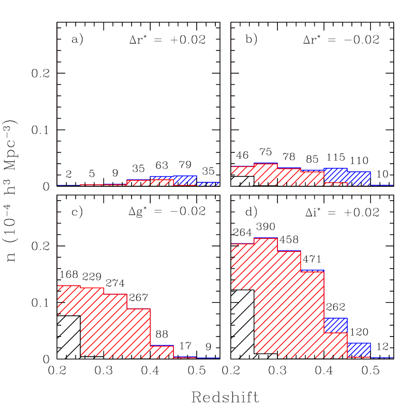
The LRG sample selection is extremely sensitive to the calibration of the $g^{*}$, $r^{*}$, and $i^{*}$ photometry. Figure 17 shows the redshift distribution of galaxies that would be excluded were the photometric zeropoints perturbed by 0.02 mag. Making $i^{*}$ fainter by 0.02 mag excludes 20% of the galaxies, while making $g^{*}$ brighter by 0.02 mag excludes 10%. Changes in $r^{*}$ exclude fewer galaxies. This sensitivity is not surprising, as one is sampling a very steep portion of the luminosity function.

Moreover, as apparent in Figure 17, changes in the photometric zeropoints interact with the selection cuts to skew the redshift distribution of the sample. Cut I is primarily affected by the shifting of $c_{\parallel}$ and $r^{*}_{\rm Petro}$ in equation (4). The effect is such that 0.01 mag in $c_{\parallel}$ or 0.03 mag in $r^{*}_{\rm Petro}$ adjusts the number density by 10%. However, to first approximation, this affects all redshifts equally as one changes the luminosity threshold.

Cut II, on the other hand, is fairly insensitive to changes in $g^{*}$ and hence to $g^{*}-r^{*}$. It is quite sensitive to $r^{*}$ and $i^{*}$ changes. The sensitive boundary here is equation (10), which separates the $z>0.4$ region from the low-redshift locus. Many Cut II galaxies are near this boundary and near the flux limit. A blue-ward shift in $r^{*}-i^{*}$ can leave galaxies outside the boundary, and if they have $19.2<r^{*}_{\rm Petro}<19.5$ then they are too faint for Cut I. On the other hand, simply moving the $r^{*}$ zeropoint fainter causes a noticeable number of Cut II objects to miss the $r^{*}_{\rm Petro}<19.5$ flux cut (Fig. 17a).

The combination of the sensitivity to certain offsets in color and the measurement errors on these colors will introduce a Malmquist-like systematic bias in the measured colors relative to the true colors. For example, the median quoted error on $c_{\parallel}$ is 0.023 mag at $r^{*}=18$ and 0.053 mag at $r^{*}=19$. A simple calculation shows that if a population of sources has a true distribution of a property $x$ proportional to $e^{-\alpha x}$ and that $x$ is measured with a Gaussian error $\sigma$, then the apparent number of sources with $x>0$ is inflated by a value $\exp(\alpha^{2}\sigma^{2}/2)$ and the distribution of true $x$ for a given observed $x$ is shifted by $-\alpha\sigma^{2}$. If $x$ is our color $c_{\parallel}$ for Cut I, then $\alpha$ is about 10 mag^-1, which means that measurement errors at $r^{*}=19$, where $\sigma\approx 0.05$, have inflated the number of targets by 13% and biased the mean color by 0.025 mag. The effects are considerably smaller at $r^{*}=18$. We have neglected these biases because they are smaller than our uncertainties in the $K+e$ corrections, but eventually a detailed analysis of the evolution of colors and number densities of LRGs will need to account for these measurement biases.

It is interesting to note that errors in the amplitude of the correction for interstellar extinction have relatively little effect on Cut I. Galaxies become both redder and fainter, and the two effects partially cancel. Of course, errors in the slope of the extinction curve would alter this balance.

5 Conclusions

The luminous red galaxy subsample of the SDSS galaxy spectroscopic survey will provide a sample of over 100,000 intrinsically luminous early-type galaxies to $z\approx 0.5$. The selection is designed to impose a passively-evolving luminosity cut so as to approach a volume-limited sample. We have demonstrated that this holds to $z=0.38$; the sample becomes flux-limited at higher redshifts because of the signal-to-noise ratio limits of the spectroscopic data. The efficiency of the selection at finding luminous early-type galaxies is very high, about 95% in Cut I and 90% in Cut II. The success rate for the spectra to yield a redshift is also very high but may drop for the faintest, highest redshift galaxies.

The primary science drivers of the LRG sample are to trace clusters of galaxies out to $z=0.5$ and to provide an enormous volume for the study of large-scale structure. It should also provide a large sample for the study of the evolution of giant ellipticals, provided that one can account for the effects of the color selection. As of June 2001, there are 15,000 unique LRGs at $z>0.2$ with survey quality data in hand, along with over 3000 duplicate observations. Thus, the SDSS LRG sample currently maps a comoving volume of about $1.5\times 10^{8}h^{-3}{\rm\,Mpc^{3}}$ with a relatively uniform set of luminous, early-type galaxies. The full sample will cover over $1h^{-3}{\rm\,Gpc^{3}}$. It is clear from the data in hand that the sample will realize its goal of providing a powerful extension of the SDSS spectroscopic survey for the study of structure and galaxy evolution at intermediate redshifts.

The Sloan Digital Sky Survey (SDSS) is a joint project of The University of Chicago, Fermilab, the Institute for Advanced Study, the Japan Participation Group, The Johns Hopkins University, the Max-Planck-Institute for Astronomy (MPIA), the Max-Planck-Institute for Astrophysics (MPA), New Mexico State University, Princeton University, the United States Naval Observatory, and the University of Washington. Apache Point Observatory, site of the SDSS telescopes, is operated by the Astrophysical Research Consortium (ARC).

Funding for the project has been provided by the Alfred P. Sloan Foundation, the SDSS member institutions, the National Aeronautics and Space Administration, the National Science Foundation, the U.S. Department of Energy, the Japanese Monbukagakusho, and the Max Planck Society. The SDSS Web site is http://www.sdss.org/.

We thank Michael Blanton, Doug Finkbeiner, and Ann Zabludoff for useful conversations, Rob Kennicutt and Rolf Jansen for supplying their spectrophotometry in electronic form, and Stéphane Charlot for supplying his latest population synthesis models. D.J.E. was supported by NASA through Hubble Fellowship grant #HF-01118.01-99A from the Space Telescope Science Institute, which is operated by the Association of Universities for Research in Astronomy, Inc, under NASA contract NAS5-26555, as well as by the Frank and Peggy Taplin Membership at the IAS.

Appendix A Target Selection in the Commissioning Data

The selection cuts described in section 2.3 are current versions and are expected to be applied throughout the remainder of the SDSS. However, the commissioning data, such as those contained in the Early Data Release (Stoughton et al., 2001), were used to refine target selection and hence applied slightly different cuts as we learned about the imaging data and the sample. These changes are tracked by the version number of target.

Working backwards in time, target versions earlier than v2_13_4 (chunks 4 to 9, tiles 73 to 219) used a value of 0.3 in the Cut II star-galaxy cut (eq. [13]). Note that this yields a superset of the current selection, so one can easily restore the current selection. target versions earlier than v2_9 (chunks 4 to 8, tiles 73 to 205) used a value of 1.35 in the Cut II equation (11) and did not apply the $r^{*}-i^{*}<1.5$ cut. target versions earlier than v2_7 (chunks 4 to 7, tiles 73 to 159) applied a Cut II surface brightness cut (eq. [12]) of 23.3 rather than 24.2; this eliminates about 15% of the objects that would now pass Cut II.

Finally, prior to target v2_7 (chunks 4 to 7, tiles 73 to 159), both cuts used the photo variable objc_type equal to 3 for star-galaxy separation, replacing equations (8) and (13). Note that this is the only change to Cut I, but it has no effect on completeness: since the change, no Cut I object and only one Cut II object that turned out to have a non-stellar redshift has had objc_type not equal to 3. For Cut I, only one object out of $\sim\!3000$ in Chunks 4 to 7 failed equation (8). Hence, for Cut I, the change in star-galaxy separation did not affect the selection of galaxies in any important way. For Cut II, about 1% of galaxies in Chunks 4 to 9 fail equation (13). The change in the star-galaxy separation cut did somewhat affect the fraction of stellar interlopers and there are stars that pass the objc_type cut and fail the $r^{*}_{\rm psf}-r^{*}_{\rm model}$ cut and vice versa. The variable objc_type was eliminated from the selection to remove dependences on the $u$ and $z$ bands.

It is important to note that the evolution of the photo pipeline could also affect the selection function. In particular, changes in the measurement of model magnitudes and the parameters of the deblending algorithm may cause subtle differences in the performance of LRG selection between different chunks. We have not yet studied these issues. The photometric calibration of the commissioning data was also preliminary; this may affect the selection in the manner displayed in Figure 17.

For completeness, we note that the now-obsolete chunk 2 used a completely different set of LRG cuts that we will not document here. This portion of sky was re-targeted as chunk 8.

Appendix B $K$-corrections and Passive Evolution

Because the LRG sample spans a wide range of redshifts, the interpretations of the sample often require the application of $K$-corrections and stellar population evolution corrections for comparison of photometry at different redshifts. While $K$-corrections alone could be derived empirically from spectrophotometry, evolutionary corrections necessarily require models. In this paper, we use models based on the PEGASE stellar population model (Fioc & Rocca-Volmerange, 1997) to derive a set of $K+e$ corrections.

If we only wanted to estimate the passively-evolved absolute magnitude for an old stellar population, then we could rely on a single star formation history, namely an old single burst. However, because we also want to investigate the dispersion in rest-frame colors, we need to specify a range of star formation histories.

At the typical redshift of the LRG sample, the observed $g$ and $r$ bands are close to the rest-frame $u$ and $g$ bands, respectively. Hence, we use $r^{*}_{\rm Petro}$ to predict the rest-frame $g^{*}_{\rm Petro}$ magnitude. For colors, however, we use the observed $g^{*}-i^{*}$ color to predict the rest-frame $u^{*}-g^{*}$ color; we pick the wider baseline so as to avoid concerns about the 4000Å band being in the $r$ band at the higher redshift end of the sample.

Figure 18: Median observed colors of LRGs in a series of redshift bins. (black) Each dot indicates the median colors within a slice of $\Delta z=0.02$. Larger dots are slices centered at $z=0.2$, 0.3, 0.4, and 0.5 (blue to red); smaller dots are centered every 0.02. (red) Crosses mark the predicted color of an old stellar population as described in Appendix B.

Figure 19: As Figure 18, but the axes have been rotated to the $c_{\parallel}$–$c_{\perp}$ system.

Table 1:

Colors and $K$-corrections for two evolving galaxy models
Non-star-forming Star-forming $z$ $\Delta g^{*}$ $u^{*}-g^{*}$ $g^{*}-r^{*}$ $r^{*}-i^{*}$ $\Delta g^{*}$ $u^{*}-g^{*}$ $g^{*}-r^{*}$ $r^{*}-i^{*}$ 0.00 0.000 1.929 0.775 0.387 0.000 1.758 0.727 0.374 0.02 0.039 1.928 0.810 0.389 0.034 1.754 0.759 0.375 0.04 0.081 1.940 0.843 0.403 0.071 1.757 0.788 0.388 0.06 0.128 1.955 0.881 0.417 0.113 1.756 0.822 0.401 0.08 0.182 1.965 0.924 0.432 0.161 1.748 0.860 0.415 0.10 0.249 1.961 0.977 0.440 0.221 1.727 0.907 0.421 0.12 0.322 1.957 1.036 0.451 0.286 1.704 0.960 0.432 0.14 0.402 1.953 1.102 0.469 0.358 1.677 1.019 0.448 0.16 0.487 1.957 1.173 0.486 0.433 1.655 1.082 0.464 0.18 0.575 1.964 1.249 0.499 0.511 1.631 1.149 0.475 0.20 0.665 1.969 1.328 0.515 0.591 1.603 1.218 0.489 0.22 0.752 1.976 1.400 0.533 0.666 1.575 1.281 0.505 0.24 0.836 1.995 1.475 0.542 0.738 1.552 1.345 0.513 0.26 0.912 2.030 1.533 0.553 0.804 1.535 1.397 0.522 0.28 0.980 2.069 1.583 0.568 0.865 1.517 1.440 0.535 0.30 1.056 2.109 1.642 0.581 0.929 1.494 1.491 0.545 0.32 1.146 2.147 1.719 0.588 1.005 1.459 1.555 0.551 0.34 1.233 2.185 1.778 0.605 1.077 1.421 1.604 0.565 0.36 1.285 2.248 1.800 0.618 1.120 1.402 1.621 0.575 0.38 1.322 2.312 1.805 0.637 1.150 1.383 1.623 0.591 0.40 1.350 2.386 1.792 0.671 1.172 1.369 1.609 0.621 0.42 1.382 2.461 1.767 0.718 1.194 1.352 1.582 0.662 0.44 1.433 2.541 1.755 0.773 1.229 1.327 1.561 0.711 0.46 1.484 2.628 1.737 0.836 1.261 1.300 1.532 0.768 0.48 1.535 2.703 1.715 0.905 1.293 1.267 1.499 0.831 0.50 1.584 2.750 1.684 0.971 1.322 1.227 1.458 0.891 0.52 1.634 2.773 1.657 1.039 1.350 1.181 1.419 0.953 0.54 1.692 2.774 1.642 1.096 1.384 1.127 1.388 1.005 0.56 1.747 2.770 1.629 1.151 1.414 1.075 1.358 1.055 0.58 1.808 2.763 1.626 1.194 1.447 1.020 1.335 1.095 0.60 1.881 2.746 1.637 1.236 1.486 0.959 1.320 1.134

NOTES—To convert from observed $r^{*}$ to $z=0$ $M_{g}^{*}$, one must subtract the distance modulus and the value in the $\Delta g^{*}$ column and add the value in the $g^{*}-r^{*}$ column, all for the redshift in question. We linearly interpolate between these two models based on the observed $g^{*}-i^{*}$ color of a galaxy at its spectroscopic redshift. Note that the models have been altered by 0.08 mag blueward in $g^{*}-r^{*}$. This correction is appropriate to the photometric calibrations applied in Stoughton et al. (2001), but the models will need to be revisited when new calibrations become available.

Figure 20: (top panel) The comparison of observed $g^{*}-r^{*}$ color to rest-frame $u^{*}-r^{*}$ color as a function of redshift for a set of non-evolving galaxy models. The models are derived from the PEGASE code and span a wide range of rest-frame colors; the reddest model is marked with the large dots. (bottom panel) As before, but for observed $r^{*}$ magnitude compared to rest-frame $g^{*}$ magnitude. We have added a $2.5\log(1+z)$ term so that a perfectly rescaled filter band would have zero offset in magnitude; this is required because the definition of the $AB_{95}$ normalization is in energy per unit frequency (Fukugita et al., 1996). For both the colors and magnitudes, one sees that the transformation from observed $g^{*}$ and $r^{*}$ to rest-frame $u^{*}$ and $g^{*}$ is insensitive to the galaxy SED at $z\approx 0.32$.

Figure 21: The rest-frame $u^{*}-g^{*}$ color and absolute $g^{*}$ magnitude for LRGs with redshifts between 0.30 and 0.35. In this range, the uncertainties of the $K$-corrections are quite small. No evolution correction has been applied, and the magnitudes of the models are not adjusted by the 0.08 mag in $g^{*}-r^{*}$ used elsewhere in the paper. SDSS calibration uncertainties could still shift the locus.

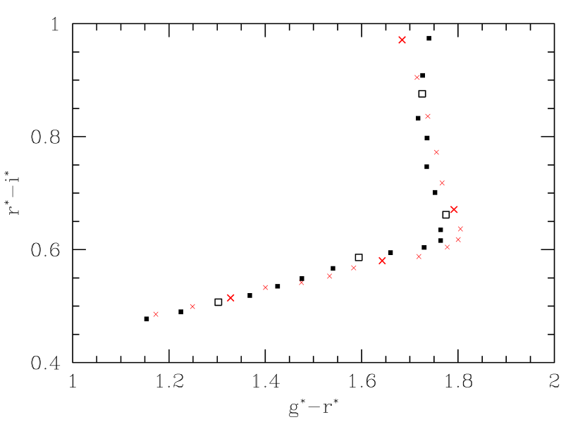
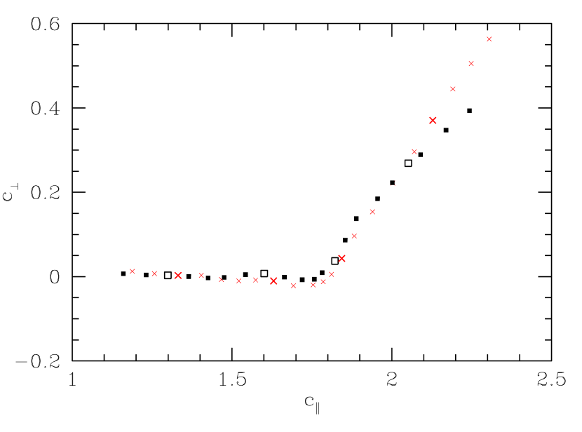
We construct two evolving stellar synthesis models from the PEGASE code. One is an old, passively evolving burst from $z\approx 10$; the other is a old population that quickly forms new stars from the mass loss of existing stars. Both assume solar metallicity for all stars and a Salpeter initial mass function. Broadband colors are calculated using the system response measured for the SDSS (Stoughton et al., 2001). At any given redshift, the second model is bluer than the first. We therefore take the redshift of an LRG and select the linear combination of the two models that matches the predicted $g^{*}-i^{*}$ color at that redshift to the observed color. This gives us an effective type, from which we quote the $K+e$ corrections to the magnitude and color at $z=0$.

We have encountered a persistent problem that all model spectra and external spectrophotometry of elliptical galaxies (e.g. Coleman et al., 1980; Kennicutt, 1992; Jansen, 2000) that we have tried predict $g^{*}-r^{*}$ colors that are significantly redder (typically about 0.1 mag) than the SDSS data. There could be at least three causes: the current SDSS photometric calibrations of one or more bands are not on the $AB_{95}$ system, the assumed system response curves are inaccurate in some way, or the external spectrophotometry has broad-band discrepancies. However, if the stellar population synthesis models have such residuals, then the redshifting of these patterns through the filter bands makes it difficult to detect errors in the evolution assumptions. We do suspect that the SDSS calibration is imperfect but not to the extent needed to reconcile the galaxy colors. As a result of the uncertainties in the calibration and the models, we cannot quote a set of $K+e$ corrections to the precision needed to compare the $z=0.4$ galaxies in the LRG sample to the $z=0.1$ galaxies in the MAIN sample.

To reconcile the observed color-redshift relation with the two models used to generate $K+e$ corrections, we subtract 0.08 mag from the $g^{*}-r^{*}$ color of the model galaxies. This puts the bluer model at the lower envelope of the LRG color data as a function of redshift. It is important to note that this affects the reconstruction of the rest-frame $u^{*}-g^{*}$ color more than the absolute $g^{*}$ magnitude. The $K+e$ corrections to the absolute magnitude in the two models differ by at most 2%, but leaving out the color shift causes a noticeable (and non-monotonic) trend in rest-frame color versus redshift. With the shift, the trend is much smaller but not absent.

Figure 18 shows the observed color-redshift relation for LRGs as compared to the redder model. Each point marks the median color in $g^{*}-r^{*}$ and $r^{*}-i^{*}$ for a shell in redshift of 0.02 width. Figure 19 shows the same figure rotated to the $c_{\parallel}$-$c_{\perp}$ plane.

While we hope that the modeling of the galaxy colors will improve in the future, Table 1 presents the colors and magnitudes of the two models used here (including the 0.08 mag shift) so that the reader can reproduce the figures in this paper as desired. For reference, the primordial burst model evolves 0.10 mag in rest-frame $u^{*}-g^{*}$ and 0.38 mag in rest-frame $g^{*}$ between $z=0$ and $z=0.35$.

We have tried other evolution models for old stellar populations, including different parameter sets within PEGASE and models from Bruzual & Charlot (2001). We find that the models generally predict similar amounts of luminosity evolution, such that we estimate the systematic uncertainty in $M_{g}^{*}$ at $z=0$ to be about 0.1 mag. However, the models do predict different color-redshift loci, such that one could mask or mimic a substantial evolution in color between $z\approx 0.4$ and today. This does not affect the interpretations of rest-frame color presented in this paper (e.g. the fact that intrinsically bluer galaxies must be more luminous to pass Cut I), but those who intend to use the sample to study galaxy evolution will need to confront this issue.

In Figure 11, we placed the low-redshift MAIN galaxies on the $M_{g}^{*}$ versus rest-frame $u^{*}-g^{*}$ plane by applying $K+e$ corrections to the observed $g^{*}$ magnitude and $u^{*}-g^{*}$ color (unlike the LRGs, the bright MAIN galaxies have well-measured $u^{*}$ magnitudes).

As a separate exercise, we can minimize our dependence on the modeling by focusing on a special redshift region. It turns out that the spacing of the $u^{*}$, $g^{*}$, and $r^{*}$ filters is such at $z\approx 0.32$ the effective wavelengths of $g^{*}$ and $r^{*}$ are nearly equal to those of rest-frame $u^{*}$ and $g^{*}$. This means that the observed $g^{*}-r^{*}$ color will predict rest-frame $u^{*}-g^{*}$ with little dependence on the SED of the galaxy. In Figure 20, we compare the observed colors to the rest-frame colors (assuming an ${\rm AB}_{95}$ zeropoint) for a variety of PEGASE models spanning a wide range of star formation histories. In detail, the $g^{*}$ filter is fractionally wider than the other two bands, which produces a $\sim\!0.05$ mag offset between $g^{*}-r^{*}$ and rest-frame $u^{*}-g^{*}$. One can see that at $z\approx 0.32$, the variation in SEDs makes rather little difference to the conversion to the rest-frame quantities.

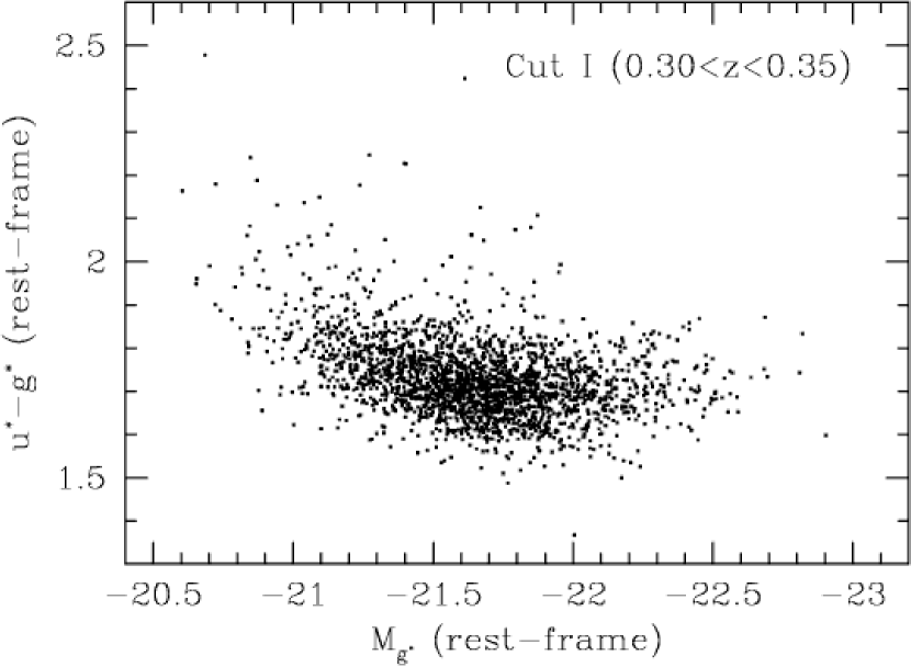
In Figure 21, we use the observed $g^{*}-r^{*}$ color and $r^{*}_{\rm Petro}$ magnitude to calculate the rest-frame $u^{*}-g^{*}$ color versus absolute $g^{*}$ magnitude for Cut I LRGs with redshifts between $0.3$ and $0.35$. Here, we do not use evolving models nor do we apply the 0.08 mag shift in $g^{*}-r^{*}$ color. The Figure therefore shows where LRGs lie in rest-frame color-magnitude space at $z\approx 0.32$. Note that to compare to lower redshift data, one would have to take account of both evolution and any possible errors in the SDSS photometric zeropoints.

References

- Annis et al. (1999) Annis, J., Kent, S., Castander, F., Eisenstein, D., Gunn, J., Kim, R., Lupton, R., Nichol, R., Postman, M., Voges, W., 1999, BAAS, 195, 1202
- Aragón-Salamanca et al. (1993) Aragón-Salamanca, A., Ellis, R.S., Couch, W.J., & Carter, D., 1993, MNRAS, 262, 764
- Aragón-Salamanca et al. (1998) Aragón-Salamanca A., Baugh, C.M., Kauffmann, G., 1998, MNRAS, 297, 427
- Baum (1962) Baum, W.A., 1962, Problems of Extragactic Research, IAU Symposium 15, 390
- Blanton et al. (2001) Blanton, M.R., et al., 2001a, AJ, 121, 2358
- Blanton et al. (2001) Blanton, M.R., Lupton, R.H., Maley, F.M., Young, N., Zehavi, I., Loveday, J., 2001b, AJ, submitted
- Bruzual & Charlot (2001) Bruzual A., G., & Charlot, S., 2001, in preparation
- Burke et al. (2000) Burke, D.J., Collins, C.A., & Mann, R.G., 2000, ApJ, 532, L105
- Castander et al. (2001) Castander, F.J., et al., 2001, AJ, 121, 2331
- Coleman et al. (1980) Coleman, G.D., Wu, C.-C., Weedman, D.W., 1980, ApJS, 43, 393
- Collins & Mann (1998) Collins, C.A., & Mann, R.G., 1998, MNRAS, 297, 128
- Connolly et al. (1995) Connolly, A.J., Csabai, I., Szalay, A.S., Koo, D.C., Kron, R.G., & Munn, J A., 1995 AJ, 110, 2655
- Dressler & Gunn (1983) Dressler, A., & Gunn, J.E., 1983, ApJ, 270, 7
- Ellis et al. (1997) Ellis, R.S., Smail, I., Dressler, A., Oemler Jr., A., Bucher, H., & Sharples, R.M., 1997, ApJ, 483, 582
- Fan et al. (2001) Fan, X., et al., AJ, 121, 31
- Fioc & Rocca-Volmerange (1997) Fioc, M., & Rocca-Volmerange, B., 1997, A&A, 326, 950
- Frieman et al. (2001) Frieman, J., et al., 2001, in preparation
- Fukugita et al. (1995) Fukugita, M., Shimasaku, K., Ichikawa, T., 1995, PASP, 107, 945
- Fukugita et al. (1996) Fukugita, M., Ichikawa, T., Gunn, J.E., Doi, M., Shimasaku, K., & Schneider, D.P., 1996, AJ, 111, 1748
- Gladders & Yee (2000) Gladders, M.D., & Yee, H.K.C., 2000, AJ, 120, 2148
- Goto et al. (2001) Goto, T., et al., 2001, in preparation
- Gunn & Oke (1975) Gunn, J.E., & Oke, J.B., 1975, ApJ, 195, 255
- Gunn et al. (1998) Gunn, J.E., et al., 1998, AJ, 116, 3040
- Hoessel et al. (1980) Hoessel, J.G., Gunn, J.E., Thuan, T.X., 1980, ApJ, 241, 486
- Jansen (2000) Jansen, R.A., Fabricant, D., Franx, M., Caldwell, N., 2000, ApJS, 126, 331
- Kauffmann (1996) Kauffmann, G., 1996, MNRAS, 281, 487
- Kauffmann et al. (1996) Kauffmann, G., Charlot, S., & White, S.D.M., 1996, MNRAS, 283, L117
- Kennicutt (1992) Kennicutt, R.C., 1992, ApJS, 79, 255
- Kim et al. (2001) Kim, R.S.J., Kepner, J.V., Postman, M., Strauss, M.A., Bahcall, N.A., Gunn, J.E., Lupton, R.H., Annis, J., Nichol, B., Castander, F.J., Brinkmann, J., Brunner, R.J., Connolly, A., Csabai, I., Hindsley, R.B., Ivezić, Ž., Vogeley, M.S., & York, D.G., 2000, AJ, submitted
- Koo (1985) Koo, D.C., 1985, AJ, 90, 418
- Loh & Spillar (1986) Loh, E.D., & Spillar, E.J., 1986, ApJ, 303, 154
- Lubin (1996) Lubin, L.M., 1996, AJ, 112, 23
- Lupton et al. (2001a) Lupton, R., Gunn, J.E., Ivezić, Z., Knapp, G.R., Kent, S., & Yasuda, N. 2001, in ASP Conf. Ser. 238, Astronomical Data Analysis Software and Systems X, ed. F. R. Harnden, Jr., F. A. Primini, and H. E. Payne (San Francisco: Astr. Spc. Pac.), in press; astro-ph/0101420
- Lupton et al. (2001b) Lupton, R.H. et al., 2001, in preparation
- Nichol et al. (2000) Nichol, B., et al., 2000, in “Mining the Sky”, MPA/MPE/ESO Conference Proceedings; astro-ph/0011557
- Oke et al. (1996) Oke, J.B., Gunn, J.E., & Hoessel, J.G., 1996, AJ, 111, 29
- Oke & Sandage (1968) Oke, J.B., & Sandage, A., 1968, ApJ, 154, 21
- Petrosian (1976) Petrosian, V., 1976, ApJ, 209, L1
- Postman & Lauer (1995) Postman, M. & Lauer, T.R., 1995, ApJ, 440, 28
- Rakos & Schombert (1995) Rakos, K.D. & Schombert, J.M., 1995, ApJ, 439, 47
- Sandage (1972) Sandage, A., 1972, ApJ, 178, 1
- Schild & Oke (1971) Schild, R., & Oke, J.B., 1971, ApJ, 169, 209
- Schlegel et al. (1998) Schlegel, D.J., Finkbeiner, D.P., Davis, M., 1998, ApJ, 500, 525
- Schlegel et al. (2001a) Schlegel, D.J., et al., 2001a, in preparation
- Schlegel et al. (2001b) Schlegel, D.J., et al., 2001b, in preparation
- Schneider et al. (1983) Schneider, D.P., Gunn, J.E., Hoessel, J.G., 1983, ApJ, 264, 337
- Stanford et al. (1998) Stanford, S.A., Eisenhardt, P.R., & Dickinson, M., 1998, ApJ, 492, 461
- Stoughton et al. (2001) Stoughton, C., et al., 2001, AJ, in preparation
- Strauss et al. (2001) Strauss, M.A., et al., 2001, in preparation
- Uomoto et al. (2001) Uomoto, A., et al., 2001, in preparation
- van Dokkum et al. (1998) van Dokkum, P.G., Franx, M., Kelson, D.D., & Illingworth, G.D., 1998 ApJ, 504, L17
- Warren et al. (1993) Warren, S.J., Hewett, P.C., Lewis, G.F., Møller, P., Iovino, A., Shaver, P.A., 1993, in ASP Conference Series 51: Observational Cosmology, eds. G. Chincarini, A. Iovino, T. Maccacaro, and D. Maccagini (San Francisco)
- Wilson et al. (2001) Wilson, G., Kaiser, N., Luppino, G.A., & Cowie, L.L. 2001, ApJ, 555, 572
- York et al. (2000) York, D., et al., 2000, AJ, 120, 1579