Physical properties and small-scale structure of the Lyman-$\alpha$ forest: Inversion of the HE 1122$-$1628 UVES spectrum

We study the physical properties of the Lyman-$\alpha$ forest by applying the inversion method described by Pichon et al. (2001) to the high resolution and high S/N ratio spectrum of the $z_{\rm em}$ = 2.40 quasar HE 1122$-$1628 obtained during Science Verification of UVES at the VLT. We compare the column densities obtained with the new fitting procedure with those derived using standard Voigt profile methods. The agreement is good and gives confidence in the new description of the Lyman-$\alpha$ forest as a continuous field as derived from our method. We show that the observed number density of lines with log $N$ $>$ 13 and 14 is, respectively, 50 and 250 per unit redshift at $z$ $\sim$ 2. We study the physical state of the gas, neglecting peculiar velocities, assuming a relation between the overdensity and the temperature. $T$ = ${\overline{T}}(\rho(x)/{\bar{\rho}})^{2\beta}$. There is an intrinsic degeneracy between the parameters $\beta$ and ${\overline{T}}$. We demonstrate that, at a fixed $\beta$, the temperature at mean density, ${\overline{T}}$, can be uniquely extracted, however. While applying the method to HE 1122$-$1628, we conclude that for 0.2 $<$ $\beta$ $<$ 0.3, 6000 $<$ ${\overline{T}}$ $<$ 15000 K at $z$ $\sim$ 2. We investigate the small-scale structure of strong absorption lines using the information derived from the Lyman-$\beta$, Lyman-$\gamma$ and C iv profiles. Introducing the Lyman-$\beta$ line in the fit allows us to reconstruct the density field up to $\rho/{\bar{\rho}}$ $\sim$ 10 instead of 5 for the Lyman-$\alpha$ line only. The neutral hydrogen density is of the order of $\sim$2$\times$10^-9 cm^-3 and the C iv/H i ratio varies from about 0.001 to 0.01 within the complexes of total column density $N$(H i) $\sim$ 10¹⁵ cm^-2. Such numbers are expected for photo-ionized gas of density $n_{\rm H}$ $\sim$ 10^-4 cm^-3 and [C/H] $\sim$ $-$2.5. There may be small velocity shifts ($\sim$10 km s^-1) between the peaks in the C iv and H i density profiles. Although the statistics is small, it seems that C iv/H i and $n_{\rm HI}$ are anti-correlated. This could be a consequence of the high sensitivity of the C iv/H i ratio to temperature. The presence of associated O vi absorption, with a similar profile, confirms that the gas is photo-ionized and at a temperature of $T$ $\sim$ 10⁵ K.

1 Introduction

The numerous absorption lines seen in the spectra of distant quasars (the so-called Lyman-$\alpha$ forest) reveal the intergalactic medium (IGM) up to redshifts larger than 5. It is believed that the space distribution of the gas traces the potential wells of the dark matter. Indeed, recent numerical $N$-body simulations have been successful at reproducing the observed characteristics of the Lyman-$\alpha$ forest (Cen et al. 1994, Petitjean et al. 1995, Hernquist et al. 1996, Zhang et al. 1995, Mücket et al. 1996, Miralda-Escudé et al. 1996, Bond & Wadsley 1998). The IGM is therefore seen as a smooth pervasive medium which can be used to study the spatial distribution of the mass on scales larger than the Jeans’ length. This idea is reinforced by observations of multiple lines of sight. It is observed that the Lyman-$\alpha$ forest is fairly homogeneous on scales smaller than 100 kpc (Smette et al. 1995, Impey et al. 1996) and highly correlated on scales up to one megaparsec (Dinshaw et al. 1995, Fang et al. 1996, Petitjean et al. 1998, Crotts & Fang 1998, D’Odorico et al. 1998, Young et al. 2001). The number of known suitable multiple lines of sight is small, however, and the sample need to be significantly enlarged before any firm conclusion can be drawn.

The standard method to analyze the observed Lyman-$\alpha$ forest is to fit the spectra as a superposition of Voigt profiles (e.g. Carswell et al. 1987). The IGM is then described as a juxtaposition of discrete clouds rather than a continuous field. Very recently, new methods have been implemented to recover the real space density distribution of the IGM by inversion of the Lyman-$\alpha$ forest. Nusser & Haehnelt (1999, 2000) proposed an iterative scheme based on Lucy’s deconvolution method (Lucy 1974). Pichon et al. (2001) used a general non-linear explicit Bayesian deconvolution method which offers the possibility to add as much a priori information as is available. The method has been implemented in order to recover the 3D topology of the large-scale structures when applied to the inversion of a network of adjacent lines of sight.

Here we apply this method to invert a high S/N ratio and high resolution spectrum of HE 1122$-$1628 obtained with UVES at ESO and therefore investigate the physical conditions of the IGM at $z$ $\sim$ 2. Data are presented in Section 2. The assumed model for the Lyman absorption is described in Section 3. The method is sketched in Appendix B. In Section 4 we investigate how the method can be used to constrain the temperature-density relation in the IGM and apply it to HE 1122$-$1628. Section 5 is dedicated to a comparison between a traditionnal Voigt profile decomposition and our method. In Section 6 we use the additional information provided by higher Lyman series absorption profiles to deconvolve the saturated Lyman-$\alpha$ lines. We use this information to investigate the C iv/H i ratio through high density profiles . We finally draw our conclusions in Section 7

2 Data

The $m_{\rm V}$ = 15.5 and $z_{\rm em}$ = 2.40 quasar HE 1122$-$1628 was observed during Science Verification of the Ultra-violet and Visible Echelle Spectrograph mounted on the 8.2 m Kuyen telescope of the European Southern Observatory, mount Paranal (Chile). The spectrum, made public by ESO, was reduced and normalized by Cédric Ledoux using MIDAS, the ESO data reduction package and following the pipeline step by step. Metals were identified and flagged when redshifted in the Lyman-$\alpha$ forest before any fitting procedure was applied. Table A.1 gives the results (position, Doppler parameter and column densities) of fitting the Lyman-$\alpha$ forest of HE 1122-1622 with two methods: (i) an automatic Voigt profile procedure (Carswell et al. 1987) and (ii) the Bayesian inversion method (see below and Pichon et al. 2001 for details). The redshift range probed by the spectrum is $1.86-2.38$ for the Lyman-$\alpha$ forest and $2.-2.38$ for the Lyman-$\alpha$ and Lyman-$\beta$ forests.

In the course of the study, we use three synthetic spectra, F₁, F₂ and F₃. The spectra were generated analytically applying the procedure described by Bi & Davidsen (1997) and using a temperature-density relation (see Eq. 2) with $\beta=0.25$ and $\overline{T}$ = 10 000, 20 000 and 30 000 K, respectively (see Choudhury et al. 2001). Photon and pixel noise is added in such a way that the signal-to-noise ratio is 50, corresponding approximately to the quality of the observed spectrum.

3 The Bayesian inversion method

We inverse the observed Lyman-$\alpha$ forest for the density field using a Bayesian method. This method is a generalisation of Wiener filtering, which is capable of dealing with a non-linear model for the Lyman-$\alpha$ absorption, including for instance the effects of gas temperature and of peculiar motions. In this study, we assume the model described below, in which peculiar motions are neglected.

The optical depth, $\tau$, in the Lyman-$\alpha$ forest is

$$\tau(w)=\frac{c\,\sigma_{0}}{H(\overline{z})\sqrt{\pi}}\int_{-\infty}^{+\infty}\frac{n_{{\rm HI}}(x)}{b(x)}\exp\left(-\frac{(w-x)^{2}}{b(x)^{2}}\right){{\mathrm{d}}{x}}\,,$$ (1)

where $c$ is the velocity of light, $\sigma_{0}$ is the Lyman-$\alpha$ absorption cross section, $H$ is the Hubble constant at redshift $\overline{z}$, $n_{{\rm HI}}$ the H i density field and $b$ the Doppler parameter. $\omega$ and $x$ are velocities (in km s^-1). The observed flux, $F$, is simply $F=\exp(-\tau)$. We use $H_{0}$ = 75 km/s/Mpc throughout the paper.

Following Hui & Gnedin (1997), we assume a temperature-density relation

$$T=\overline{T}\left(\frac{\rho_{\rm DM}({\mathbf{x}})}{\bar{\rho}_{\rm DM}}\right)^{\gamma-1}\,,$$ (2)

where $\overline{T}$ is the temperature at mean dark matter density, $\bar{\rho}_{\rm DM}$, and $\gamma-1$ is the polytropic index. And therefore,

$$\ \ b({\mathbf{x}})=13\,{\rm kms^{-1}}\ \sqrt{\frac{\overline{T}}{10^{4}K}}\left(\frac{\rho_{\rm DM}({\mathbf{x}})}{\bar{\rho}_{\rm DM}}\right)^{\beta}\,,$$ (3)

where $\gamma-1=2\beta$.

A simple functional relation between the dark matter density $\rho_{\rm DM}$ and the neutral hydrogen particle density $n_{\rm HI}$ is assumed,

$$\ \ n_{\rm HI}({\mathbf{x}})=\overline{n}_{\rm HI}\left(\frac{\rho_{\rm DM}({\mathbf{x}})}{\bar{\rho}_{\rm DM}}\right)^{\alpha}\,,$$ (4)

where $\alpha=2\mbox{--}1.4\times\beta$. Eq. 1 reads

$$\tau(w) = A(\overline{z})c_{1}\int_{-\infty}^{+\infty}\left(\frac{\rho_{\rm DM}(x)}{\bar{\rho}_{\rm DM}}\right)^{\alpha-\beta}$$ (5)

$$\ \ \times\ \exp\left(-c_{2}\frac{(w-x)^{2}}{\left[{\rho_{\rm DM}(x)}/{\bar{\rho}_{\rm DM}}\right]^{2\beta}}\right){{\mathrm{d}}{x}}\,.$$

The parameters $c_{1}$, $c_{2}$ and $A(\overline{z})$ depends on the characteristic temperature of the IGM

$$\ \ c_{1}=\left(13\sqrt{\pi}\sqrt{\frac{\overline{T}}{10^{4}}}\right)^{-1},\quad c_{2}=\left(13^{2}\frac{\overline{T}}{10^{4}}\right)^{-1}$$ (6)

$$\mathrm{and\ \ }A(\overline{z})=\frac{\overline{n}_{\rm HI}\,c\,\sigma_{0}}{H(\overline{z})}\propto\ \frac{{\overline{T}}^{-0.7}}{J}\,,$$

where $J$ is the ionizing flux, assumed to be uniform. $A(\overline{z})$ is chosen in order to match the observed average optical depth of the Lyman-$\alpha$ forest ($\simeq$ 0.2 at $z$ = 2). In the case of HE 1122$-$1628, we measure ${\cal A}(\overline{z})=0.22$ in the UVES spectrum and therefore use this value in the following.

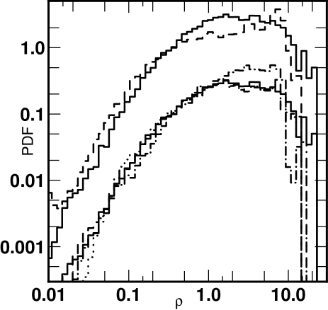
We assume that the a priori density obeys a lognormal distribution characterised by its a priori correlation matrix. We plot in Fig. 1 the PDF of the analytical density field used to generate spectrum F₁ (solid line; the peculiar velocities are not considered) together with the PDF reconstructed after inversion of F₁ (dashed and dotted lines for S/N ratios of 50 and 1000 respectively). Overplotted as a dashed line, but shifted by a factor of ten for clarity, is the PDF for the HE 1122$-$168 spectrum. This justifies the lognormal approximation. The discrepancy beyond $\rho/{\bar{\rho}}$ $\sim$ 1 is due to redshift distortion (see Nusser et al., 2000).

The sought parameters, ${\mathbf{M}}$, are the logarithm of the continuous field $\rho_{\rm DM}/\bar{\rho}_{\rm DM}$ (named $p$ in the following), together with the two parameters of Eq. 2, $\overline{T}$ and $\beta$. The priors of the inversion are described by the above equations 2, 3, 4, plus a probability distribution of ${\mathbf{M}}$, involving a prior guess ${\mathbf{M}}_{0}$ and a correlation function ${\mathbf{C}}_{0}$ for $p$

$${\mathbf{C}}_{0_{i,j}}=\sigma_{p}\ \times\ \exp\left(-\frac{(x_{i}-x_{j})^{2}}{\xi_{r}^{2}}\right)\,.$$ (7)

In this work, ${\mathbf{M}}_{0}\equiv\left(p_{0}=0,\ \overline{T}{\rm\ and\ }\beta{\rm\ fixed}\right)$. The model that relates the data ${\mathbf{D}}$ and the parameters ${\mathbf{M}}$ is given by Eq. 5.

Figure 1: Simulated and reconstructed probability Distribution Function (PDF), $\rho\ P(\log(\rho))$, of the over-density $\rho/{\bar{\rho}}$. The simulated density PDF is plotted as a solid line. From this density, a spectrum has been generated in real space and thermally broadened. Different amounts of noise have been added. The density field is then recovered using the inversion technique described in Section 3. The dotted and dashed lines correspond to the PDF of the density recovered from spectra with a S/N ratio of 50 and 1000, respectively. The two PDFs are approximately the same except for the low density region. Noise induces a lower and an upper cutoff in the recovered PDF. The PDF in the redshift-space spectrum is shown as a dot-dashed line. The PDF recovered from the UVES spectrum scaled up by a factor of 10 for clarity, is shown as another dashed line. The density PDF in the simulation is plotted with the same scaling, upper solid line, to aid the comparison.

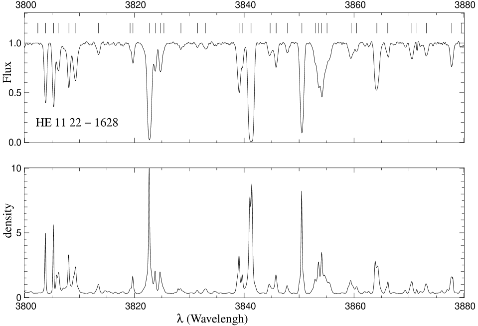
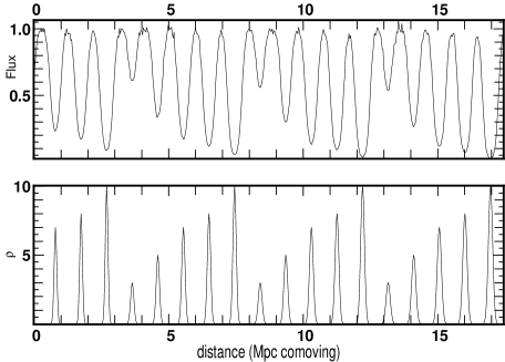
An example of the reconstruction is given in Fig. 2 which shows part of the spectrum of HE 1122$-$1628 (upper panel) and the reconstructed density (lower panel).

Figure 2: Portion of the spectrum of HE 1122$-$1628 (upper panel) and corresponding reconstructed DM density (bottom panel) when peculiar velocities are not considered. The vertical marks indicate the positions of individual components found by the automatic Voigt profile fitting procedure. The S/N ratio in the data is of the order of 60 per pixel.

4 Constraining the temperature at mean density

The method described in Section 3 is applied to the spectrum of HE 1122$-$1628 to constrain the parameters of the temperature-density relation : the exponent $\beta$ and the temperature at the mean density $\overline{T}$ (see Eq. 2). The inversion is performed for a grid of $\beta$ and $\overline{T}$ values. Following Hui & Gnedin (1997), we restrict our study to $\beta$ in the range 0.2–0.3.

Figure 3: Result of the fit of a synthetic spectrum constructed from an analytical simulation and assuming an temperature-density relation defined by Eq. 2 with $\beta_{0}$ = 0.25 and $\overline{T}_{0}$ = 10 000 K (spectrum F₁, see Section 2). The inversion is performed for the density field, for a grid of couples ($\beta$,$\overline{T}$), and the final minimum reduced $\chi^{2}$ is plotted versus $\beta$ and $\overline{T}$. The plane corresponding to $\chi^{2}=1$ is shown with dotted lines. The locus of the points ($\beta$,$\overline{T}$,$\chi^{2}$=1) is what is refered to as the borderline in the text. The correct couple ($\beta_{0}$, $\overline{T}_{0}$), marked by a filled square, is located on this borderline.

Figure 4: Result of the fit of a synthetic spectrum constructed from a simple 1D density field (Fig A.2) and assuming a temperature-density relation defined by Eq. 2 with $\beta_{0}$ = 0.25 and $\overline{T}_{0}$ = 10 000 K. The inversion is performed for the density field, for different values of $\overline{T}$ while $\beta=\beta_{0}$ is fixed. The final minimum reduced $\chi^{2}$ is plotted versus $\overline{T}$. The horizontal and vertical dotted lines correspond to $\chi^{2}=1$ and $\overline{T}=\overline{T}_{0}$ respectively. The intersection of the curves with the $\chi^{2}$=1 line defines the borderline. The different curves correspond to different values of the priors as defined by the matrix ${\mathbf{C}}_{0}$, i.e. its variance $\sigma_{p}$ and correlation length, $\xi_{r}$ (see Section 3). $\xi_{r}=0.12-0.55$ Mpc comoving (top to bottom panel) and $\sigma_{p}=0.2-0.5$ (solid and dashed lines). In this range, the value of $\overline{T}$ on the borderline is constant within $10\%$.

4.1 Application to synthetic spectra

4.1.1 Definition of a borderline in the ($\beta$,$\overline{T}$) plane

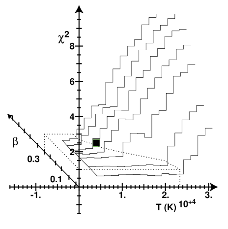
We first try to recover the initial couple ($\beta_{0}$,$\overline{T}_{0}$) used to generate one of the synthetic spectra (see Section 2). For this, we fix a couple ($\beta$,$\overline{T}$) and inverse the spectrum for the density field. We derive the minimum reduced $\chi^{2}$ value obtained by fitting the model to the data, i.e. $({\mathbf{D}}-g({\mathbf{M}}))^{\perp}.{\mathbf{C}}_{d}^{-1}.({\mathbf{D}}-g({\mathbf{M}}))$, see Section 3. The result of fitting the synthetic spectrum F₁ is shown in Fig. 3. The ($\beta$,$\overline{T}$) plane is divided into two regions with, respectively, $\chi^{2}$ $<$ 1 and $\chi^{2}$ $>$ 1, separated by a well-defined approximately straight borderline. The correct value of $\overline{T}$ lies on the $\chi^{2}=1$ borderline. This is expected as explained in Appendix A.

We have investigated the dependance of the position of this borderline with respect to the parameters of the inversion, namely the correlation amplitude ($\sigma_{p}$) and correlation length ($\xi_{r}$) of the prior matrix ${\mathbf{C}}_{0}$. $\xi_{r}$ should be of the order of the spectral resolution (here, the pixel corresponds to 0.05 Å  or 0.047 Mpc comoving) ; $\sigma_{p}$ controls the fluctuations of the density between two iterations. $\sigma_{p}$ should be neither too small to allow for the recovery of the high density peaks, nor too large for stability of the algorithm. It can be seen in Fig. 4 that for $0.2\leq\sigma_{p}\leq 0.5$ and $0.12\leq\xi_{r}({\rm Mpc\ com.})\leq 0.55$, the $\chi^{2}=1$ border corresponds to the same $\overline{T}$ within $10\%$. We use $\sigma_{p}=0.25{\rm\ and\ }\xi_{r}=0.2$.

Note, however, that a high $\chi^{2}$ value can be the consequence of only a small portion of the spectrum beeing poorly fitted. This implies that, when fitting real data, the borderline can be considered as a lower limit for the temperature at fixed $\beta$.

It remains that the inversion problem is degenerate: it is always possible to find a good fit to the data with any given value of $\beta$ provided $\overline{T}$ is changed. We have tried to find a systematic approach to be able to recover from the synthetic data the temperature at mean density $\overline{T}$ that was used to create the data.

4.1.2 Where is the strongest constraint on $\overline{T}$ ?

Zaldarriaga et al. (2000) have shown that the flux power spectrum is affected by changes in the temperature only for overdensities between 0.9 and 1.8. It is likely that not all the absorption features are well suited to constrain the temperature and one can wonder which features constrain the temperature best. Indeed, low density regions are associated with diffuse gas in voids where temperature broadening is washed out by the smoothness of the density field itself. This suggests that the strongest constraint on the temperature determination comes from moderately saturated lines.

To check this, we divided the spectrum in sub-spectra, of typical width 20 Å. In each sub-spectrum we define the maximum optical depth, $\tau_{\rm max}$, corresponding to a normalized flux $F_{\rm min}$. As argued previously, it is expected that the sub-spectra where $F_{\rm min}$ is large will poorly constrain the temperature. We therefore limit the inversion to sub-spectra where some condition on $F_{\rm min}$ is imposed. We have checked that the width of the sub-spectra is not a critical parameter for the procedure. It must be large enough to include an important range of apparent optical depths but not too large, in order to keep enough weight on large optical depths.

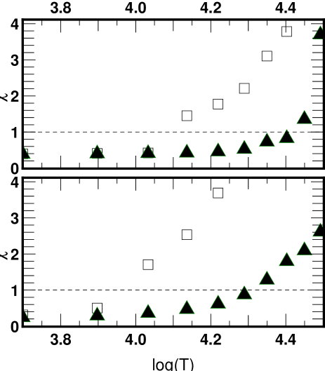
Fig. 5 shows the results of the inversion of the sub-spectra of the synthetic spectrum F1, varying $\overline{T}$ while keeping $\beta$ equal to 0.25 (which is the correct initial value). The reduced $\chi^{2}$ is plotted versus the mean temperature for $F_{\rm min}$ $<0.1$ (only strong features are considered; results are shown as open squares in the figure) and for 0.2 $<$ $F_{\rm min}$ $<0.3$ (lines of intermediate saturation only are considered; results are shown as filled triangles in the figure). It is apparent that, for weak lines, $\chi^{2}$ remains smaller than one for a very wide range of temperatures. Instead, for strong lines, $\chi^{2}$ is larger than one for all temperatures larger than the correct value $\overline{T}$ = 10⁴ K. Note that a normalized flux of 0.2 corresponds to an overdensity of $\rho/{\bar{\rho}}\sim\leavevmode\nobreak\ 2$. Because of this behaviour, only sub-spectra with $F_{\rm min}$ $<0.2$ are used in the following to constrain $\overline{T}$.

4.1.3 Estimation of the temperature $\overline{T}$

The reduced $\chi^{2}$ is computed for each sub-spectrum, labelled $i$, and each couple ($\beta$,$\overline{T}$). This defines the temperature on the borderline, $\overline{T}_{\rm\beta,i}$, for each sub-spectrum. The highest $\overline{T}_{\rm\beta,i}$ correspond to segments where the density field is so smoothed that the effect of temperature is very small. This introduces a systematic bias against low temperatures.

Using the synthetic spectrum, we check that, for the correct value of $\beta$, an appropriate estimator of $\overline{T}_{0}$ is the median of the $1^{\rm st}$ quartile of the cumulative distribution, $P(\overline{T})$, defined as the region where $0.<P(\overline{T})<0.25$. This is illustrated in Fig. 6 where this estimator of $\overline{T}_{0}$ is plotted versus $\beta$ for the three synthetic spectra F1 (10 000 K), F2 (20 000 K) and F3 (30 000 K). The error bars represent the range of temperatures in the $1^{\rm st}$ quartile. The three initial temperatures are recovered with this estimator for the correct value of $\beta$ = 0.25.

Figure 5: Minimum reduced $\chi^{2}$ versus log $\overline{T}$ obtained after fitting 20 Å  wide portions of the synthetic spectrum F₁ (upper panel) or of the HE 1128$-$1628 spectrum (lower panel). The portions are chosen so that the minimum value of the normalized flux is smaller than 0.1 (open squares) or is in the range 0.2$-$0.3 (filled triangles). The reconstruction is performed for $\beta$ = 0.25. Note that in the simulation (upper panel), $\overline{T}$ = 10000 K.

Figure 6: Recovered parameters of the temperature-density relation for different analytical spectra. Each of the spectra are generated using the same density field and $\beta$ = 0.25 but with three different temperatures: $\overline{T}=10\,000\ {\rm K}\ {\rm(circles),\ }20\,000\ {\rm K}\ {\rm(squares),\ }30\,000\ {\rm K}\ {\rm(crosses)}$. Results from inversions are shown as open symbols; the initial parameters are shown as filled symbols. See text for the definition of the estimator. The largest uncertainty in the determination of the absolute temperature from the inversion comes from the degeneracy between $\beta$ and $\overline{T}$.

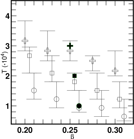
4.2 Application to HE 1122$-$1628 and discussion

The same procedure is applied to the UVES spectrum of HE 1122$-$1628. It can be seen in Fig. 5 (lower panel) that, as already noted with analytical data, the fit of strong lines is more constraining than the fit of weak lines.

Results on the determination of $\overline{T}$ along the line of sight to HE 1122$-$1628 is given in Fig. 7. This figure (when compared to Fig. 6) suggests that the temperature of the IGM at mean density at redshift $z$ $\sim$ 2 is only slightly larger than 10⁴ K. Accounting for the uncertainty due to the inherent lack of knowledge on $\beta$, we conclude that $\overline{T}$ $\sim$ 10000${}_{6000}^{15000}$ K at $z$ = 2.

Figure 7: Parameters of the temperature-density relation recovered by inversion of the UVES spectrum of HE 1122-1628. The temperature at mean density at z $\simeq 2$ is found in the range 6 000$-$15 000 K. The trend shown in this figure is close to that found in the F1 spectrum (see Fig. 6) where $\overline{T}$=10 000 K.

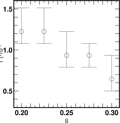
Other methods have been applied to determine the temperature-density relation of the IGM over the past few years. Schaye et al. (2000), Ricotti et al. (2000) and Mc Donald et al. (2000) deconvolve the spectra using Voigt profile fitting. They then consider that the temperature can be estimated from the lower bound of the locus of observed values of the Doppler parameter and neutral hydrogen column density. This is reminiscent of the reasoning used by Pettini et al. (1990). The three groups derive similar results. For an average redshift of 2.4, they find, respectively, $\overline{T}/10^{4}=0.8-2$, $\beta=0.25\pm 0.07$; $\overline{T}/10^{4}=0.7-5$ and $\beta=0-0.3$ and $\overline{T}/10^{4}=1.74\pm 0.19$ and $\beta=0.26\pm 0.07$ . As emphasized by Zaldarriaga et al. (2000), these authors use a lower limit of the width of the lines over the whole spectrum. They therefore derive a lower limit on the temperature. Another approach that does not make use of any fitting procedure has been developed by Zaldarriaga et al. (2000). It relies on the determination of the flux power-spectrum. These authors show that there is no power on scales smaller than the scale corresponding to thermal broadening $b_{\rm T}$. They find, for the same redshift, $\overline{T}(\beta=0)/10^{4}=1.8-3.2$ and $\overline{T}(\beta=0.3)/10^{4}=1.-1.6$. All analyses show a dependance of $\overline{T}$ over $\beta$ similar to that shown in Fig. 7.

In addition, Hui & Gnedin (1997) conclude from the results of hydro-simulations that $\overline{T}\ {\rm and}\ \beta$ reach an asymptotic value at low redshift: $\overline{T}\propto\left(\frac{\Omega_{b}\ h^{2}}{\sqrt{\Omega_{m}\ h^{2}}}\right)^{1/1.7}$ and $\beta>0.15\ -0.24\$, depending on the exact reionization history. This corresponds approximately to a temperature at overdensity unity that decreases from about 10 000 K at $z=4$ to 8000 K at $z=2$. Note however that they did not include the effects of He ii reionisation.

Our findings are therefore consistent with previous published analysis. Note that the remaining discrepancies in the results obtained by the various authors could be a consequence of the fact that a single temperature-density relation is assumed for the gas. In particular, it is probable that spatial variations of the ionizing flux can have a substantial influence on the temperature (see e.g. Zaldarriaga 2001). It should be possible to investigate this in more detail using our procedure if a large number of lines of sight is observed at the same resolution and S/N ratio. Such data will be available after a few years of observations with UVES at the VLT. Moreover, the determination of the characteristic temperature of the IGM over a large redshift range could constrain the reionisation history. Indeed, Schaye et al. (2000) have tentatively found a peak of $T$ = $10^{4.4}$ K at a redshift of 3.2 (compared to about $10^{4}$ K at redshifts 3.5 and 2) and interpret this as evidence for He ii reionisation.

5 Comparison with Voigt profile fitting

In this Section, we compare the column densities evaluated along the line of sight to HE 1122$-$1628 from the fit of the Lyman-$\alpha$ forest using the inversion method on the one hand and VPFIT, the automatic Voigt profile procedure (Carswell et al. 1987) on the other hand. The latter procedure decomposes the spectrum in discrete absorption components, whose Doppler parameters and column densities are fitted to the data. Our method derives the density in each velocity pixel and we must integrate this density over some velocity range, chosen somewhat arbitrarily, to recover a column density and compare it to VPFIT’s. At the position of each cloud defined by VPFIT, we integrate over twice the Doppler parameter of the cloud. Table A.1 summarizes the results.

Fig. 8 shows the histograms of the values taken by the ratio between the two column densities when only the Lyman-$\alpha$ line is considered (solid line) and when the Lyman-$\beta$ line is used in addition to constrain the fit (dashed line). The mean difference between the two estimations is about 15%, well within the uncertainties due to the measurements themselves. The inversion method usually underestimates the high column densities. This is a consequence of the lack of information in the saturated part of the corresponding absorption lines. In addition, the fact that the procedure reconstructs a continuous field minimizes the importance of the wings of the line. The situation is improved, as expected, when the Lyman$-\beta$ line is used to constrain the fit. The mean difference is then reduced to about 10%.

The improvement in the inversion of the density field when including the Lyman-$\beta$ forest is emphasized in Fig. 9. We inverse one of the synthetic spectra for which we know the real overdensity in each pixel. Fig. 9 gives the reconstructed overdensity versus the overdensity used to simulate the spectrum. When the Lyman-$\alpha$ line only is used, the density field is recovered up to overdensities slightly larger than 5, whereas when the Lyman-$\beta$ forest is used in addition, overdensities up to 10 are recovered.

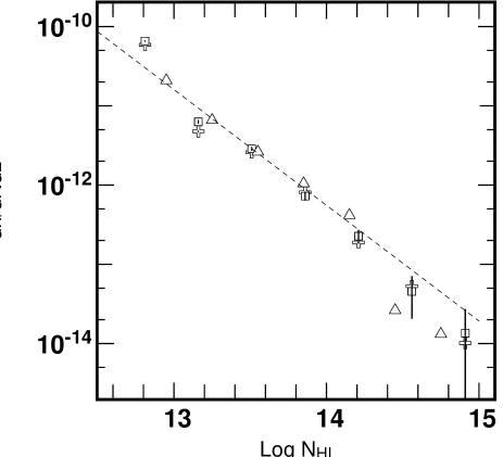
Fig. 10 shows the H i column density distribution derived from the inversion of the Lyman-$\alpha$ and Lyman-$\beta$ forests observed toward HE 1122$-$1628 together with the results from the automatic fitting of the Lyman-$\alpha$ forest using VPFIT and the data points from Kim et al. (1997). A correction has been applied at the low column density end to take into account incompleteness induced by the blending of weak lines with strong ones (Kim et al. 1997). There is a remarkable agreement between the inversion method, VPFIT and previous observations.

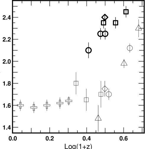
The number of absorption lines per unit redshift is given in Fig. 11 as a function of redshift. Although  previous analyses have concentrated on strong lines, log $N$(H i) $>$ 14, most of the constraints on the IGM come from weaker lines. Our results at $z$ $\sim$ 2 for log $N$(H i) $>$ 13 and log $N$(H i) $>$ 14, together with other observational points (Giallongo et al. 1996, Kim et al. 1997, Weymann et al. 1998, Savaglio et al. 1999, Kim et al. 2000), nicely fall on top of the predictions by Riediger et al. (1998).

Figure 8: Histogram of the difference between the logarithm of the H i column densities obtained using the Voigt profile fitting procedure ($N_{\rm fit}$) on the one hand, and the inversion method ($N_{\rm rec}$) on the other hand, from the fit of the Lyman-$\alpha$ forest only (solid line) or for both the Lyman-$\alpha$ and Lyman-$\beta$ forests (dashed line), evaluated along the line of sight to HE 1122-1628. For the inversion procedure, the column densities are estimated by integrating the recovered density over twice the Doppler parameter found by the Voigt profile fit.

Figure 9: Over-densities recovered after inversion of a synthetic spectrum versus the over-densities used to generate the synthetic spectrum, assuming $\overline{T}=10^{4}{\rm K},\beta=0.25$.

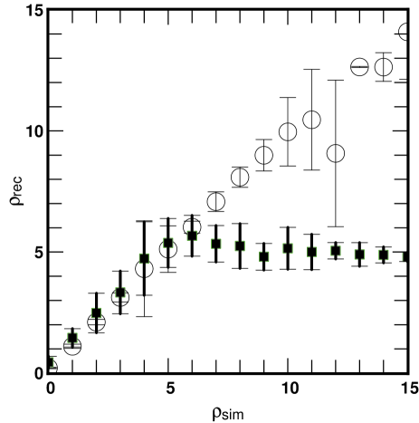
When only Lyman-$\alpha$ data is available for the inversion procedure (filled squares), overdensities larger than 5 cannot be recovered because of saturation effects. This situation is very much improved when using the Lyman-$\beta$ forest data (open circles).

Figure 10: Column density distribution at z $\simeq$ 2.3, corrected for incompleteness, as measured toward HE 1122-1628 from the inversion procedure (crosses) and the Voigt profile procedure (squares). Also plotted is the distribution obtained by Kim et al. (1997, triangles).

Figure 11: Number density of lines versus redshift for different column density thresholds: log $N$(H i) $>$ 13 (Kim et al. 1997, thick squares; Kim et al. 2000, thick circles; this work, thick losange), log $N$(H i) $>$ 14 (Savaglio et al. 1999, squares); Weymann et al. 1998, crosses; Kim et al. 1997, circles; Giallongo et al. 1996, triangles; this work, losange).

In this Section, we have not yet taken advantage of the true capabilities of the Bayesian method. Indeed, we first inverted the spectrum to a density field and then reprojected the result into discrete clouds. In the following, we concentrate on other questions, taking full advantage of the new method.

6 Structures in the strong lines

As long as only unsaturated lines are considered, the corresponding structures are clearly identified in the spectrum. The same structures are lost, however, when blended with saturated lines whose width is often of the order of 100 km s^-1 (see below). The nature of the strong lines (log $N$(H i) $>$ 14) is unclear and they could be associated with filaments, halos with rotation velocities less than about 100 km s^-1 and/or external regions of galactic halos (see e.g. Mücket et al. 1996). Observations of adjacent lines of sight have concluded that these lines arise in complexes with transverse dimensions larger than 200 kpc. To gain insight into the small-scale structure of these complexes, we can try to invert the corresponding Lyman-$\alpha$ lines, adding information from all observed lines in the Lyman series and when available from the associated C iv lines. The inversion is performed in redshift space.

6.1 Inversion of strong lines

We have selected for further analysis the 12 lines seen in the spectrum of HE 1122$-$1628 which have log $N$(H i) $>$ 14 and a large enough redshift ($z_{\rm abs}$ $>$ 2.03) so that the Lyman-$\beta$ line is redshifted in the observed wavelength range. A more accurate Voigt profile fit has been performed on these individual lines, including whenever possible other lines in the Lyman series (mostly Lyman-$\beta$ and Lyman-$\gamma$). Also, we have inverted the flux with the Bayesian method including all pieces of information available. Since the associated C iv lines are most of the time too weak, we do not include the C iv profile as a constraint for the inversion and keep it instead for an a-posteriori discussion of the C iv/H i ratio.

Figure 12: Example of the inversion of a saturated line, using both the Lyman-$\alpha$ and Lyman-$\beta$ profiles. The temperature-density relation used during inversion is defined by $\beta=0.25$ and $\overline{T}=8\,000$ K (Eq. 2). The recovered density is shown in the bottom panel. The other panels shows from bottom to top the Lyman-$\alpha$, Lyman-$\beta$, C iv$\lambda$1548 and C iv$\lambda$1550 profiles. The reconstructed flux after inversion is overplotted as dashed lines. Note that the blending of the Lyman-$\beta$ forest is ignored by the inversion. Vertical lines show the position of components identified by the Voigt profile fitting procedure.

Figure 13: Same as Fig. 12 for another system. Here $\overline{T}=11000$ K. Note that the density is reconstructed even where the Lyman-$\alpha$ forest is saturated, thanks to the constraints from the Lyman-$\beta$ forest.

Figure 14: Illustration of the influence of the a-priori correlation length (see text) and the temperature-density relation on the recovered density in the Lyman-$\alpha$ complex at $\lambda$ $\sim$4076 Å  (see also Fig. 16). Top panel: Lyman-$\alpha$, Lyman-$\beta$ and C iv absorption profiles are shown as, respectively, solid, dashed and dotted lines. Middle panel: recovered density for different correlation lengths, 0.05 Å (dashed line) and 0.1-0.2 Å (solid line, both profiles are undistinguishable). Note that the pixel size is 0.05 Å. Bottom panel: recovered density for three different values of the temperature-density relation parameters; the three ($\beta$,$\overline{T}$) couples are on the borderline defined in Fig. 7: solid line, $\beta=0.2,\ \overline{T}=15\,000$ K, dashed line, $\beta=0.25,\ \overline{T}=10\,000$ K, dotted line, $\beta=0.3,\ \overline{T}=5\,000$ K.

Figure 15: Two-point correlation functions of the flux in HE 1122$-$1628 at $z$ $\sim$ 2. (light solid lines); the three lines correspond to the function itself and the function $\pm$1$\sigma$. The dashed lines correspond to the measurements by McDonald et al. (2000) at $z$ = 3.89, 3.0 and 2.41 are shown as, respectively dashed, dotted and dash-dotted lines. The thick solid line is the function calculated for the recovered density.

In principle, the Lyman-$\beta$ line can always be blended with an intervening Lyman-$\alpha$ line at lower redshift. We therefore define

$$\tau_{Ly\beta}={\rm min}(\tau_{z\beta},\tau_{z\alpha}*f_{\alpha}\lambda_{\alpha}/f_{\beta}\lambda_{\beta}),$$ (8)

where $\tau_{z\beta}$ and $\tau_{z\alpha}$ are the observed optical depth at the position of the Lyman-$\beta$ and Lyman-$\alpha$ absorptions respectively; $f_{\alpha}$, $f_{\beta}$, $\lambda_{\alpha}$ and $\lambda_{\beta}$ are the oscillator strengths and rest-wavelengths of the Lyman-$\alpha$ and Lyman-$\beta$ lines. We then invert $\tau_{Ly\beta}\ {\rm and\ }\tau_{Ly\alpha}$ simultaneously (with the same relative weight for the two lines).

Figure 16: Same as Fig. 12 for the complex at $\lambda$4076 Å. The C iv is strong enough to allow us to study the ratio C iv/H i (Fig. 17). Note the shift between the H i and C iv strongest peaks (the position of the density peaks does not depend strongly on the parameters of the inversion, see Fig. 14). Note also the presence of C iv in the wings of H i profile (at $\lambda\sim$ 4076.5 Å, marker B in Fig. 17). The O vi profile is also shown in the upper panel. The similarity of the O vi and C iv profiles is a signature of predominance of photo-ionization in the ionization balance.

Figure 17: Determination of the C iv/H i ratio along the absorption profile of the strong complex at $\lambda$4076 Å (see also Fig. 16). Bottom panel: Lyman-$\alpha$ (solid line), Lyman-$\beta$ (dashed line) and C iv (scaled by a factor 4, dotted line) absorption profiles. Second panel: recovered H i (solid line) and C iv (scaled by the average C iv/H i ratio, dashed line) density (see text for details about the reconstruction). Third panel: C iv/H i ratio; the horizontal line indicates the ratio of the C iv and H i integrated densities. Top panel: the C iv/H i ratio is plotted versus the H i density. The markers A and B correspond to positions discussed in the text.

Figure 18: Same as Fig. 16 for the complex at $\lambda$4096 Å.

Figure 19: Same as Fig. 17 for the complex at $\lambda$4096 Å (see also Fig. 18).

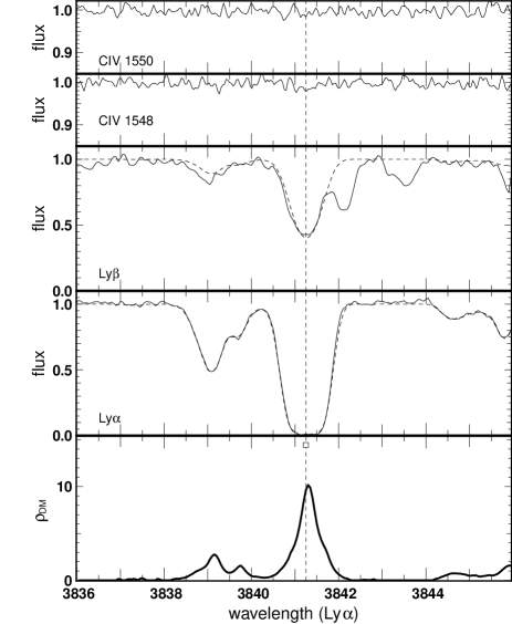
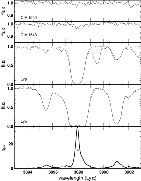
A few examples of the fits and reconstructions are given in Figs 12,13,16,18. From bottom to top, the different panels correspond to (i) the reconstructed density, (ii) the Lyman-$\alpha$ absorption profile, (iii) the Lyman-$\beta$ or the Lyman-$\gamma$ profiles, (iv) the associated C iv$\lambda\lambda$1548,1550 doublet and (v) when possible, the associated O vi absorption. The fit models are overplotted on the observed Lyman profiles as dashed lines. The positions of the components used in the Voigt profile fits are marked by vertical lines.

6.2 Validation

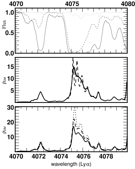
The inversion procedure uses a correlation length to propagate the information along the line of sight. It is important to check the robustness of the results when changing this parameter. For this, we invert the Lyman-$\alpha$ structure at 4075 Å different correlation lengths (see Fig. 14, middle panel). We use the Lyman-$\beta$ and Lyman-$\alpha$ profiles to constrain the fit. It can be seen that for correlation lengths larger than the resolution of the spectrum ($\sim$0.1 Å  at this wavelength), the results are weakly dependent on the exact value of the parameter. It is only for very small correlation lengths (the pixel size is 0.05 Å), that the structures become artificially peaked. In the following, we always use a correlation length of 0.2 Å.

As the temperature-density relation is determined for the whole spectrum, it is possible that the global solution is not representative of the physical state of the gas in one particular place. To estimate the influence of a possible variation of the temperature-density relation from one place to the other, we have inverted the same Lyman-$\alpha$ feature at 4075 Å  using three different values of the couple ($\beta$,$\overline{T}$), found on the borderline defined in Section 4. Note that the values used for the three inversions are extreme and correspond to variations of a factor of three in $\beta$ and $\overline{T}$. It can be seen in Fig. 14 (bottom panel) that although the absolute amplitude of the density field varies by a factor of $\sim$2 from one inversion to the other, the shapes of the density profiles are very similar and all the structures are recovered.

6.3 Correlation function

The two-point correlation function is defined as,

$$\xi(\Delta v)=<\delta F(v)\delta F(v+\Delta v)>.$$ (9)

The function computed for the density field reconstructed from the inversion of the HE 1122$-$1628 spectrum is plotted in Fig. 15 together with the correlation function of the flux. The curves are normalized to $\xi(0)=1$. To compute errors, we used the bootstrap method presented in, e.g., McDonald et al. (1999) and found that the correlation function is not corrupted by the amount of noise. On small scales, the shape of the function is probably related to the internal structure of the Lyman-$\alpha$ clouds (or more realistically Lyman-$\alpha$ complexes), the dimension of which is expected from $N$-body simulations to be of the order of 1 Mpc ($\simeq\leavevmode\nobreak\ 130\ {\rm km\ s}^{-1}$). Observations of adjacent lines of sight also indicate that the absorptions are correlated on scales of the order of 0.2 to 1 Mpc (e.g. Petitjean et al. 1998, D’Odorico et al. 1998, Dinshaw et al. 1998, Crotts & Fang 1998). However, it must be noted that the radius derived from analysis of the metal lines associated with the Lyman-$\alpha$ forest are much smaller (Hu et al. 1995; see next Section).

6.4 The C iv/H i ratio

The determination of the amount of metals present in the Lyman-$\alpha$ forest attracts much interest because this is a key issue for understanding how the first objects in the Universe were formed. Since the first observations of metals (mostly C iv) in at least half of the Lyman-$\alpha$ lines with log $N$(H i) $>$ 14.3 (Cowie et al. 1995, Songaila & Cowie 1996), efforts have been concentrated towards constraining the metal content of the gas with smaller column densities. As direct detection of the corresponding very weak C iv lines is difficult even if the physical conditions are the same at different column densities, a statistical approach has been used. Ellison et al. (1999, 2000) conclude that observations are consistent with a constant C iv/H i $\sim$ $2\times 10^{-3}$ ratio down to very small column densities. Deriving a carbon metallicity from this is quite uncertain, however. Using hydro-simulations including photo-ionization, Rauch et al. (1997) claim that at $z$ = 3, the column density ratios of the different ionic species can be well reproduced if a mean metallicity of [Z/H] = $-$2.5 is assumed.

Out of the 12 clouds with $N$(H i) $>$ 10¹⁴ cm^-2 seen toward HE 1122$-$1628, 7 (60%) have associated C iv absorption. The average C iv/H i ratio computed after Voigt profile fitting of the absorptions is $4\times 10^{-3}$. The optical depth ratio $\tau_{\rm CIV}$/$\tau_{\rm HI}$, where $\tau_{\rm CIV}\ {\rm and\ \tau_{HI}}$ are defined as in Eq. 8 for all available components is approcimately constant and corresponds to C iv/H i$\simeq 2.5\ 10^{-3}$ for $\tau_{\rm HI}>1$ and slightly smaller for $\tau_{\rm HI}<1$.

It has already been noted by Songaila & Cowie (1996) that the C iv/H i ratio is not constant within a strong complex and seems to be larger in the wings of the strong lines. Using the inversion method we are in a position to study the variations of the C iv/H i ratio within the strong complexes. For this we must invert, not only the Lyman series as described above but also the C iv absorption. Unfortunately, due to the faintness of the C iv absorptions, the required S/N ratio is very large. Although the S/N ratio of the HE 1122$-$1628 spectrum is very good, it is high enough only for the $z_{\rm abs}$ = 2.35 and $z_{\rm abs}$ = 2.37 systems (see Figs. 17,19). We invert the absorptions for the H i density using Lyman-$\alpha$,$\beta$ for the 4076 Å complex and Lyman-$\alpha$,$\beta$,$\gamma$ for the 4096 Å complex. The C iv density is obtained from the C iv$\lambda\lambda$1548,1550 doublet. The H i particle density is of the order of 10^-9 cm^-3 which is what is expected from simulations (typically $n_{\rm H}$ $\sim$ 10^-4 cm^-3 and H i/H $\sim$ 10^-5, see e.g. Bi & Davidsen 1997, Hellsten et al. 1997). It must be noted however that this number is obtained assuming that the density is constant over the pixel size, $\simeq$ 12 kpc at $z$ = 2. The C iv/H i ratio varies from about 0.001 to 0.01 within the complexes. Finally, it can be seen that there are slight velocity shifts ($\sim$10 km s^-1) between the peaks in the C iv and H i density profiles.

The most interesting observation, however, is that there is some hint of an anti-correlation between C iv/H i and $n_{\rm HI}$ (see Figs. 17,19 upper panel where the C iv/H i ratio is plotted versus the H i density). It is difficult to assess the anti-correlation as the S/N ratio in the C iv profile is probably not high enough and more important, the statistics are poor. However, it is apparent on the profiles that (i) the strongest H i components have C iv/H i $\sim$ a few 10^-3 (e.g. region A) and (ii) there is gas in the wing of the profiles of lower H i optical depth and much larger C iv/H i ratio (e.g. region B). A straightforward interpretation would be that the carbon metallicity is not homogeneous in the cloud. A more simple explanation however is that this is a consequence of temperature fluctuations. Indeed C iv/H i is quite sensitive to the temperature for $T$ $\sim$ 10⁵ K (see e.g. Rauch et al. 1997). Because of high temperature dielectronic recombinations, C iv/H i increases with temperature. If the anti-correlation is real, this implies that the temperature of the gas increases for decreasing H i particle density and is close to 10⁵ K.

Interestingly enough, it can be noted that for collisional ionization, C iv/C has a maximum $\sim$0.35 at $T$ $\sim$ 10⁵ K (Arnaud & Rothenflug 1986) and C iv/H i $\sim$ 2$\times$10^-2 for [C/H] = 10^-2.5. However, if collisional ionization dominates, no O vi is expected in the gas, as the dominant ionization stage of oxygen is O iv at this temperature. On the contrary, in the gas we observe, it can be seen in Figs. 17,19 that O vi is indeed detected and has a similar apparent optical depth as C iv. Note that we plot in each case the line of the O vi doublet which is not blended. Moreover, as far as the S/N ratio allows the comparison, the C iv and O vi profiles are strongly correlated. This is a clear signature of the predominance of photo-ionization in the ionization balance of the gas.

7 Conclusion

We have applied the Bayesian inversion procedure developped by Pichon et al. (2001) to the high resolution and high S/N ratio spectrum of HE 1122$-$1628 obtained during Science Verification of UVES at the VLT and made publicly available by ESO. Assuming a temperature-density relation $T=\overline{T}\left(\frac{\rho_{\rm DM}({\mathbf{x}})}{\bar{\rho}_{\rm DM}}\right)^{2\beta}$ for the gas, we invert the spectrum for the density field $\rho(x)$ and recover a grid of $\chi^{2}$ versus the two parameters $\beta$ and $\overline{T}$.

We certify the method by showing that the inversion procedure applied to synthetic data enables us to infer the correct temperature when $\beta$ is given the value used to generate the data. There is an intrinsic degeneracy however between $\beta$ and $\overline{T}$ which is the source of most of the uncertainty in the determination of the temperature of the intergalactic medium. We find $\overline{T}$ $\sim$ 10000${}_{6000}^{15000}$ K at $z\sim 2$.

The results of fitting the Lyman-$\alpha$ forest with the new method or with the automatic Voigt profile fitting procedure VPFIT (Carswell et al. 1987), when expressed in terms of column densities, are found to be very similar. The new procedure however has the advantage of reconstructing the continuous density field. The latter can be recovered up to $\rho/{\bar{\rho}}$ $\sim$ 5 when the Lyman-$\alpha$ forest only is used. Above this value, saturation prevents any reliable determination of the density. Overdensities up to 10 can be recovered however when the Lyman-$\beta$ absorption is used.

We investigate the structure of the complexes with log $N$(H i) $>$ 14 by inverting the Lyman-$\alpha$ and Lyman-$\beta$ lines and therefore derive the two-point correlation function of the dark matter on scales smaller than 1 Mpc. Out of the twelve lines with log $N$(H i) $>$ 14, seven have detected associated C iv absorption. The ratio C iv/H i, derived from the optical depth ratio $\tau_{\rm CIV}$/$\tau_{\rm HI}$, is roughly constant, $\simeq 2.5\ 10^{-3}$ for $\tau_{\rm HI}>1$ and slightly smaller for $\tau_{\rm HI}<1$. In two of the complexes, we are able to inverse the C iv absorption independently. This reveals the presence of fluctuations as large as one order of magnitude in the C iv/H i ratio. This, together with the presence of O vi with the same absorption profile as C iv indicates that the gas is photo-ionized and at a temperature close to 10⁵ K.

Throughout this work, we did not take into account redshift distorsion. It is expected to modify quantitatively the result of Section 4 since the lines get thinner or broader depending of the exact distribution of the peculiar velocities. This must be investigated in detail and is beyond the scope of this paper. However, the conclusion of Section 6 about the relation between C iv and H i should be valid even in real space since velocities modify both profiles in the same way.

Appendix A Formal thermal broadening deconvolution

For a polytropic temperature-density relation, $T={{\overline{T}}{{\rho(x)}^{-2\beta}}}$, the optical depth,$\tau(w)$, is related to the underlying density via Eq. 1, where we set $A({\overline{z}})$ to 1 for simplicity. Let us explore the régime where Eq. 1 is non singular ($\beta\neq 0$). We argue here that, in this régime, at a fixed $\beta$, the inversion problem sketched in Section 4 is well paused: i.e. there is a unique solution for the underlying density field, given the measured $\tau$.

A.1 Asymptotic Expansion; Gaussian profile

Let us take the Taylor series of the integrant of Eq. 1 with respect to $\beta$

$${\frac{1}{{\sqrt{\overline{T}}}}}{{\rho(x)}^{\alpha-\beta}}\exp\Big{(}-\frac{{{(x-w)}^{2}}}{\overline{T}}{{\rho(x)}^{-2\beta}}\Big{)}\approx$$

$$\frac{{{\rho(x)}^{\alpha}}}{{\sqrt{\overline{T}}^{3}}}\exp\Big{(}-\frac{{{(w-x)}^{2}}}{\overline{T}}\Big{)}\left[{\overline{T}}-\beta{(T-2{{(w-x)}^{2}})\log(\rho(x))}\right]$$

(10)

Let us also assume for now that the underlying density field is Gaussian with an unknown rms, $\sigma_{\delta}^{2}$:

$${\rho(x)=\frac{1}{{\sqrt{2\pi}}\sigma}\exp\Big{(}-\frac{{x^{2}}}{2{{\sigma_{\delta}}^{2}}}\Big{)}}\,.$$ (11)

The optical depth associated with this density profile, Eq. 11 reads :

$${\tau(w)=\frac{{{(2\pi)}^{\frac{1-\alpha}{2}}}{{\sigma_{\delta}}^{1-\alpha}}{\exp}(-\alpha{w^{2}})}{{\sqrt{2{{\sigma_{\delta}}^{2}}+\alpha{\overline{T}}}}(2{{\sigma_{\delta}}^{2}}+\alpha{\overline{T}})}}\Big{(}\frac{P(w)\beta{\overline{T}}}{2{{\big{(}2{{\sigma_{\delta}}^{2}}+\alpha{\overline{T}}{}\big{)}}^{4}}}+1\Big{)}\,,$$ (12)

where

$$P(w) = {{{\overline{T}}}^{3}}(\log(2\pi)\alpha+1){{\alpha}^{3}}-$$ (13)

$$2{{{\overline{T}}}^{2}}\big{(}{w^{2}}+\big{(}{w^{2}}\alpha-3{{\sigma_{\delta}}^{2}}\big{)}\log(2\pi)\big{)}{{\alpha}^{3}}-$$

$${\overline{T}}{{\sigma_{\delta}}^{2}}\big{(}{w^{2}}\alpha(2\log(\pi)\alpha+\log(4)\alpha-4)-$$

$$3{{\sigma_{\delta}}^{2}}(\alpha\log(2\pi)-1)\big{)}\alpha+$$

$$2{{\big{(}2{{\sigma_{\delta}}^{2}}+{\overline{T}}\alpha\big{)}}^{2}}\big{(}-2\alpha{w^{2}}+2{{\sigma_{\delta}}^{2}}+{\overline{T}}\alpha\big{)}\log(\sigma_{\delta})\alpha-$$

$$8{{\sigma_{\delta}}^{2}}\big{(}{{\alpha}^{2}}{w^{4}}+\alpha{{\sigma_{\delta}}^{2}}(\alpha\log(2\pi)-5){w^{2}}+$$

$${{\sigma_{\delta}}^{4}}(2-\alpha\log(2\pi))\big{)}\,.$$

When $\beta\equiv 0$, the first term in the bracket of Eq. 12 vanishes; the effect of the temperature and the natural broadening of the line are degenerate, i.e. all combinations of $\sigma_{\delta}$ and ${{\overline{T}}}$ which leave ${2{{\sigma_{\delta}}^{2}}+\alpha{\overline{T}}}$ invariant give the same optical depth profile.

Thanks to Eq. 13, when $\beta\neq 0$ the shape of the line is non Gaussian, with a departure from a Gaussian distribution which is a function of the underlying temperature of the medium. This distortion is characteristic of the temperature-density relation, and can in principle be disentangled.

To demonstrate this formally, we may for instance compute the variance, ${{\sigma}_{2}}$,and the kurtosis ${{\sigma}_{4}}$, of $\tau(w)$ as a function of ${\overline{T}}$ and $\sigma_{\delta}$ (for fixed $\alpha$ and $\beta$)

$${{\sigma}_{2}} \equiv \frac{1}{\int\tau(w){\rm d}w}\int\tau(w){w^{2}}{\rm d}w$$ (14)

$$= \frac{{{\sigma_{\delta}}^{2}}}{\alpha}+{\overline{T}}\Big{(}\frac{1}{2}-\log(\sigma_{\delta})\beta-\frac{\beta}{2\alpha}-\frac{1}{2}\log(2\pi)\beta\Big{)}$$

$${{\sigma}_{4}} \equiv \frac{1}{\int\tau(w){\rm d}w}\int\tau(w){w^{4}}{\rm d}w$$ (15)

$$= \frac{3{{\sigma_{\delta}}^{4}}}{{{\alpha}^{2}}}+$$

$${{{\overline{T}}}^{2}}\Big{(}\frac{3}{4}-3\log(\sigma_{\delta})\beta-\frac{3\beta}{2\alpha}-\frac{3}{2}\log(\pi)\beta-\frac{3}{4}\log(4)\beta\Big{)}+$$

$${\overline{T}}\Big{(}\frac{3{{\sigma_{\delta}}^{2}}}{\alpha}-\frac{9\beta{{\sigma_{\delta}}^{2}}}{{{\alpha}^{2}}}-\frac{6\beta\log(\sigma_{\delta}){{\sigma_{\delta}}^{2}}}{\alpha}-\frac{3\beta\log(\pi){{\sigma_{\delta}}^{2}}}{\alpha}-$$

$$\ \ \ \ \ \ \ \ \frac{3\beta\log(16){{\sigma_{\delta}}^{2}}}{4\alpha}\Big{)}\,.$$

Solving for ${\overline{T}}$ in Eq. 14 and eliminating ${\overline{T}}$ subsequently in Eq. 15 we are left with an implicit equation for $\sigma_{\delta}[\sigma_{2},\sigma_{4},\beta,\alpha]$:

$$\big{(}6\beta(4\alpha\log(\sigma_{\delta})(\log(\sigma_{\delta})\alpha+\log(2\pi)\alpha+3)\beta+5\beta+$$

$$\alpha(\beta\log(2\pi)(\log(2\pi)\alpha+6)-4)){{\sigma_{\delta}}^{4}}+$$

$$2\alpha\big{(}-6\beta\big{(}4\alpha\log(\sigma_{\delta})(\log(\sigma_{\delta})\alpha+\log(2\pi)\alpha+2)\beta+3\beta+$$

$$\alpha\big{(}\beta\big{(}\big{(}{{\log}^{2}}(2)+\log(\pi)\log(4\pi)\big{)}\alpha+4\log(\pi)$$

$$\vspace{2cm}+\log(16)\big{)}-2\big{)}\big{)}{{\sigma}_{2}}{{\sigma_{\delta}}^{2}}+$$

$$3{{\alpha}^{2}}(4\alpha\log(\sigma_{\delta})\beta+2\beta+\alpha(2\log(\pi)\beta+\log(4)\beta-1))\sigma_{2}^{2}+$$

$$\alpha{{(2\beta\log(\sigma_{\delta})\alpha+\beta\log(2\pi)\alpha-\alpha+\beta)}^{2}}{{\sigma}_{4}}\big{)}\big{)}=0\,.$$ (16)

As expected, Eq. 16 becomes singular when $\beta=0$ i.e. it becomes: ${{{\sigma}_{4}}=3\sigma_{2}^{2}}$ (this just states that $\tau$ is also Gaussian and as such its reduced kurtosis vanishes) and does not involve $\sigma_{\delta}$ any longer. On the other hand, when $\beta\neq 0$, Eq. 16 has a solution for $\sigma_{\delta}$ and therefore for the corresponding ${\overline{T}}$ via Eq. 14. We have therefore demonstrated that it is possible to disentangle natural broadening and thermal broadening for non-singular temperature-density relations; in the limit of small $\beta$ but non-zero $\beta$.

The above argument obviously relies on the Taylor expansion, Eq. 10; we have checked that carrying the expansion to 2nd order did not qualitatively change our conclusions.

A.2 Finite signal to noise

In the presence of noise, the actual numerical inversion of a given underlying field, $\rho(x)$, remains a somewhat degenerate problem for small values of $\beta$ since the ${{\chi}^{2}}$ function will depend weakly on ${\big{(}\sigma_{\delta},{\overline{T}}\big{)}}$ near the minimum (the minimum is ”flat”). For instance, a relative error of $5\%$ on $\sigma_{2}$ and $\sigma_{4}$ leads to a relative error of $20\%$ for ${\overline{T}}$. We can use Eq. 16 to estimate what range of $\rho$ we need to consider to better constraint the temperature. A remaining issue is how does the inversion deal with lines which have intrinsic kurtosis ? It turns out that statistically (ie averaged over a few such lines) we have some insight of what the shape of the underlying density profile should be, since the relative distortions induced by $\beta$ are the same for all lines. To demonstrate this, let us investigate how our non-parametric procedure (Section 4) recovers the temperature, $\overline{T}$, for a large range of temperature (5 000 K to 30 000 K) when dealing with simulated profiles (provided the simulated data span a sufficiently large range of densities).

For this purpose, we synthetize a line of sight of H i clouds whose width and height span the range $40<\ b\ ({\rm km\ s}^{-1})\ <200$ and $3<\ \rho_{\rm max}\ <10$. This line of sight is plotted in the lower panel of Fig. 20. We generate the corresponding spectrum for ten values of $\overline{T}$ between 5 000 K and 30 000 K while $\beta$ is kept constant and equal to $0.25$. The spectrum corresponding to $\overline{T}=$15 000 K is plotted in the upper panel of Fig. 20. The recovered temperature $\overline{T}$ corresponding to a $\chi^{2}=1$ fit is plotted versus the real $\overline{T}$ in Fig. 21. For a non-parametric model, a $\chi^{2}=1\pm\sqrt{2/N}$ fit does correspond to the best estimate for the model. The temperature at mean density is better recovered for low $\overline{T}$. But the bias towards lower temperature remains small up to 30 000 K. This may be due to the increasing distance between the true density and the prior ($D_{0}$).

Figure 20: line of sight built with a wide range of density profiles (lower panel) and the corresponding spectrum computed with a temperature at mean density, $\overline{T}$, of 15 000 K and $\beta$=0.25 (upper panel). Ten spectra are computed with a range of $\overline{T}$ from 5 000 K to 30 000 K. $\overline{T}$ is then recovered with the method described in Section 4 (see Fig. 21).

Figure 21: recovered $\overline{T}$ versus real $\overline{T}$ from synthetic spectrum described in Fig. 20 ($T_{4}=\overline{T}/10^{4}$). The value of $\beta$ is assumed to be known. $\overline{T}$ is well recovered in the range 5 000 K - 30 000 K, when the data span a wide range of densities. The error bars correspond to $\chi^{2}=1\pm\sqrt{2/n}$, where n is the number of pixels. For high $\overline{T}$, there is a small bias to lower $\overline{T}$.

Appendix B The inversion technique

We aim to invert Eq. 1, i.e. reconstruct the density field $\rho_{\rm DM}$. To that end, we take a model, $g$, which basically relates the Doppler parameter $b$ and the gas density $n_{\rm HI}$ to the dark matter density, $\rho_{\rm DM}$ and the parameters of the temperature-density relation. The goal here is to determine these unknown fields, ${\mathbf{M}}=\left(\log(\frac{\rho_{\rm DM}}{\overline{\rho}_{DM}}),\overline{T},\beta\right)$, by fitting the data, ${\mathbf{D}}\equiv\tau(w_{i})$, i.e. the optical depth along the line of sight.
Since the corresponding inversion problem is under-determined, we use the Bayesian technique described in Pichon & al (2001). In order to achieve regularization, we require a prior guess for the parameters, ${\mathbf{M}}$, or in statistical terms, their probability distribution function, $f_{\rm prior}({\mathbf{M}})$. Using Bayes’ theorem, the conditional probability density $f_{\rm post}({\mathbf{M}}|{\mathbf{D}})$ for the realization ${\mathbf{M}}$ given the observed data ${\mathbf{D}}$ then writes:

$$f_{\rm post}({\mathbf{M}}|{\mathbf{D}})={\cal L}({\mathbf{D}}|{\mathbf{M}})f_{\rm prior}({\mathbf{M}})\,,$$ (17)

where $\cal L$ is the likelihood function of the data given the model. If we assume that both functions $\cal L$ and $f_{\rm prior}$ are Gaussian, we can write:

$$f_{\rm post}({\mathbf{M}}|{\mathbf{D}}) = {\cal A}\exp[-\frac{1}{2}({\mathbf{D}}-g({\mathbf{M}}))^{\perp}\cdot{\mathbf{C}}_{d}^{-1}\cdot({\mathbf{D}}-g({\mathbf{M}}))$$ (18)

$$\ -\frac{1}{2}({\mathbf{M}}-{\mathbf{M}}_{0})^{\perp}\cdot{\mathbf{C}}_{0}^{-1}\cdot({\mathbf{M}}-{\mathbf{M}}_{0})]\,,$$

with ${\mathbf{C}}_{d}$ and ${\mathbf{C}}_{0}$ being respectively the covariance “matrix” of the noise and of the prior guess for the parameters, ${\mathbf{M}}_{0}$. $\cal A$ is a normalization constant. The superscript, $\perp$, stands for transposition. In a nutshell, the minimum of the argument of the exponential in Eq. 18 is found using an iterative procedure:

$${{\mathbf{M}}}_{[k+1]} = {\mathbf{M}}_{0}+{\mathbf{C}}_{0}\cdot{{{\mathbf{G}}_{[k]}}^{\bot}}\cdot({\mathbf{C}}_{d}+{\mathbf{G}}_{[k]}\cdot{\mathbf{C}}_{0}\cdot{{{\mathbf{G}}_{[k]}}^{\bot}})^{-1}\cdot$$ (19)

$$\ \ \ \ \ \ \ ({\mathbf{D}}+{\mathbf{G}}_{[k]}\cdot({{\mathbf{M}}}_{[k]}-{\mathbf{M}}_{0})-g({{\mathbf{M}}}_{[k]}))\,,$$

where subscript $[k]$ refers to the iteration order, while ${\mathbf{G}}$ is the matrix (or more rigorously, the functional operator) of partial derivatives of the model $g({{\mathbf{M}}})$ with respect to the parameters. In this scheme the minimum corresponds to ${\mathbf{M}}_{[\infty]}$ and in practice is found via a convergence criterion on the relative changes between iteration $[k]$ and $[k+1]$.

Our model reads, Eq. 5,

$$g_{i}(p)=A(\overline{z})c_{1}\int_{-\infty}^{+\infty}(\exp[p(x)])^{\alpha-\beta}\exp\left(-c_{2}\frac{(w_{i}-x)^{2}}{(\exp[p(x)])^{2\beta}}\right){{\mathrm{d}}{x}}\,,\$$

where $p=\log(\frac{\rho_{\rm DM}}{\bar{\rho}_{\rm DM}})$. The prior is defined as ${\mathbf{M}}_{\rm 0}=(p_{0}=0)$. The treatment of the temperature-density relation is different and it is described in Section 4. Since the model, ${\mathbf{M}}\equiv p(x)$ is a continuous field, we need to interpret Eq. 19 in terms of convolutions, and functional derivatives. In particular the matrix of partial functional (Fréchet) derivatives, ${\mathbf{G}}$, has the following kernel:

$$({\mathbf{G}})_{i}(x)\equiv\left(\frac{\partial g_{i}}{\partial p}\right)(x)=A(\overline{z})c_{1}D_{0}^{\alpha-\beta}(x)\exp\left[(\alpha-\beta)p(x)\right]B_{i}(x)\,,\$$

with

$$B_{i}(x) = ((\alpha-\beta)+c_{2}2\beta(w_{i}-x)^{2}\exp\left[-2\beta p(x)\right])\cdot$$

$$\ \ \ \ \ \exp\left(-c_{2}\frac{(w_{i}-x)^{2}}{(\exp\left[p(x)\right])^{2\beta}}\right)\,.\$$