PTHalos: A fast method for generating mock galaxy distributions

Abstract

Current models of galaxy formation applied to understanding the large-scale structure of the universe have two parts. The first is an accurate solution of the equations of motion for the dark matter due to gravitational clustering. The second consists of making physically reasonable approximations to the behavior of baryons inside dark matter halos. The first uses large, computationally intensive, $n$-body simulations. We argue that because the second step is, at least at present, uncertain, it is possible to obtain similar galaxy distributions without solving the first step exactly.

We describe an algorithm which is several orders of magnitude faster than $n$-body simulations, but which is, nevertheless, rather accurate. The algorithm combines perturbation theory with virialized halo models of the nonlinear density and velocity fields. For two- and three-point statistics the resulting fields are exact on large scales, and rather accurate well into the nonlinear regime, particularly for two-point statistics in real and redshift space. We then show how to use this algorithm to generate mock galaxy distributions from halo occupation numbers. As a first application, we show that it provides a good description of the clustering of galaxies in the PSCz survey.

We also discuss applications to the estimation of non-Gaussian contributions to error bars and covariance matrix of the power spectrum, in real and redshift space, for galaxies and dark matter. The results for the latter show good agreement with simulations, supporting the use of our method to constrain cosmological parameters from upcoming galaxy surveys.

1 Introduction

Upcoming large galaxy surveys will provide a major advance in our understanding of the large-scale structure of the universe, helping to determine cosmological parameters, constrain models of galaxy formation and the properties of primordial fluctuations that gave rise to galaxies. However, extracting information about cosmological parameters from the galaxy distribution requires an accurate modeling of non-linear effects such as gravitational evolution, redshift distortions, and galaxy biasing (i.e., the relationship between the galaxy and the underlying dark matter distribution).

The physics of galaxy formation is not yet fully understood. Numerical simulations which include the effects of both gravitational instability as well as gas hydrodynamics in cosmological volumes are only now becoming available (e.g. Cen & Ostriker 2000; Pearce et al. 2001). But the role of feedback from star formation, and how to incorporate it into simulations, remains uncertain. As a result, a complementary approach to generating realistic galaxy distributions has been to use semianalytic models (see, e.g., Kauffmann et al. 1999; Somerville & Primack 1999; Cole et al. 2000).

These models build on the work of White & Rees (1978) and White & Frenk (1991), in which galaxy formation is treated as a two-stage process: dark matter haloes virialize, and gas cools and forms stars within these virialized halos. The first step is solved numerically: $n$-body simulations of nonlinear gravitational clustering are used to follow the formation of the dark matter halos. The second step uses a number of reasonable prescriptions for approximating the complicated nonlinear physics of gas cooling in gravitational potential wells to incorporate star and galaxy formation into the simulations which otherwise only describe the effects of gravitational clustering. The predictions of the semi-analytic models, while similar to those from smoothed particle simulations which solve the hydrodynamic equations for the gas numerically, can differ by as much as fifty percent in the two-point correlation function (e.g. Benson et al. 2001). Therefore, it is this second step which is the more uncertain one, since we do not yet understand galaxy formation from first principles. On the other hand, it is the first step which is the most time consuming.

In this paper we present a method which generates realistic galaxy distributions in a very small fraction of the time it takes for methods that require $n$-body simulations of gravitational clustering. By realistic distributions, we mean specifically that the point distributions our method generates can reproduce the observed galaxy clustering statistics; in particular, the distribution of galaxy counts-in-cells, the power spectrum and the bispectrum. The philosophy of our approach is that since the step which involves generating galaxies from knowledge of the dark matter distribution is necessarily uncertain, one does not need to start with a fully correct dark matter distribution to generate galaxy correlations to the extent allowed by the present understanding of galaxy formation. By suitably approximating the non-linear structures which form in the gravitational clustering simulations, one can hope to still obtain a reasonably accurate galaxy distribution by slightly altering the mapping from dark matter to galaxies within the uncertainties.

To obtain an approximation to the fully nonlinear dark matter distribution we first generate the large-scale dark matter distribution using second-order Lagrangian perturbation theory (2LPT). This reproduces the correct two and three-point statistics at large scales, and approximates the four-point and higher-order statistics very well (Moutarde et al. 1991; Buchert et al. 1994; Bouchet et al. 1995; Scoccimarro 2000). Note that use of 2LPT, rather than linear theory or the Zel’dovich approximation, is essential to incorporate accurately the large-scale departures from Gaussian initial conditions.

The 2LPT correlations are incorrect on small scales, where perturbation theory breaks down. We build up more accurate small-scale correlations by using the amplitude of the 2LPT density field to determine the masses and positions of virialized halo centers, and we then distribute particles around the halo centers with realistic density profiles. We use the 2LPT code described by Scoccimarro (1998,2000) to set up the perturbation theory density and velocity fields, and the merger history algorithm of Sheth & Lemson (1999b) to partition the 2LPT density field into haloes. Finally, a galaxy distribution can be generated by specifying how many galaxies populate haloes of a given mass (e.g. Mo, Jing & Börner 1997; Jing, Mo & Börner 1998). In this respect, our PTHalos algorithm treats the difference between the clustering statistics of the dark matter and galaxy distributions in much the same way that recent analytic models (Peacock & Smith 2000; Seljak 2000; Scoccimarro et al. 2001) do.

In this paper, we do not attempt to match other galaxy properties (e.g. the luminosity function) than clustering statistics. Statistics like the luminosity function can be estimated rather easily by simply replacing the dark matter distribution of an $n$-body simulation with the PTHalos distribution, and then running the usual semianalytic galaxy formation codes on top. Our motivation was mainly to develop a fast algorithm which can be used to generate realistic non-Gaussian galaxy distributions, and thus provide a method to quickly explore parameter space for constraining cosmological parameters and galaxy formation models from galaxy surveys. In addition, the speed of our code makes feasible to construct a large number of mock galaxy catalogs in a reasonable CPU time from which reliable estimation of errors and covariance matrices can be derived. Application along these lines to imaging data in the SDSS survey will be considered elsewhere (Connolly et al. 2001; Dodelson et al. 2001; Scranton et al. 2001; Szalay et al. 2001; Tegmark et al. 2001).

This paper is organized as follows. In Section 2 we review 2LPT. In Section 3 we describe how we parametrize haloes and in Section 4 how we place them in the 2LPT density field. In Section 5, we compare the clustering statistics of the dark matter distribution of PTHalos to $n$-body simulations. In Section 6 we describe how we map from dark matter to galaxies. We show that our method provides a sensible match to to the galaxies in the PSCz survey. We conclude in Section 7.

2 Second-Order Lagrangian PT

In Lagrangian PT, the dynamics is described by the displacement field ${\bf\Psi}({\bf q})$ which maps the initial particle positions ${\bf q}$ into the final Eulerian particle positions ${\bf x}$,

$${\bf x}={\bf q}+{\bf\Psi}({\bf q}).$$ (1)

The equation of motion for particle trajectories ${\bf x}(\tau)$ is

$$\frac{d^{2}{\bf x}}{d\tau^{2}}+{\cal H}(\tau)\ \frac{d{\bf x}}{d\tau}=-\nabla\Phi,$$ (2)

where $\Phi$ denotes the gravitational potential, and $\nabla$ the gradient operator in Eulerian coordinates ${\bf x}$. Taking the divergence of this equation we obtain

$$J({\bf q},\tau)\ \nabla\cdot\Big{[}\frac{d^{2}{\bf x}}{d\tau^{2}}+{\cal H}(\tau)\ \frac{d{\bf x}}{d\tau}\Big{]}=\frac{3}{2}\Omega_{m}{\cal H}^{2}(J-1),$$ (3)

where we have used Poisson equation together with the fact that $1+\delta({\bf x})=J^{-1}$, and the Jacobian $J({\bf q},\tau)$ is the determinant

$$J({\bf q},\tau)\equiv{\rm Det}\Big{(}\delta_{ij}+\Psi_{i,j}\Big{)},$$ (4)

where $\Psi_{i,j}\equiv\partial\Psi_{i}/\partial{\bf q}_{j}$. Equation (3) can be fully rewritten in terms of Lagrangian coordinates by using that $\nabla_{i}=(\delta_{ij}+\Psi_{i,j})^{-1}\nabla_{q_{j}}$, where $\nabla_{q}\equiv\partial/\partial{\bf q}$ denotes the gradient operator in Lagrangian coordinates. The resulting non-linear equation for ${\bf\Psi}({\bf q})$ is then solved perturbatively, expanding about its linear solution, the Zel’dovich (1970) approximation

$$\nabla_{q}\cdot{\bf\Psi}^{(1)}=-D_{1}(\tau)\ \delta({\bf q}).$$ (5)

Here $\delta({\bf q})$ denotes the (Gaussian) density field imposed by the initial conditions and $D_{1}(\tau)$ is the linear growth factor. The solution to second order describes the correction to the ZA displacement due to gravitational tidal effects and reads

$$\nabla_{q}\cdot{\bf\Psi}^{(2)}=\frac{1}{2}D_{2}(\tau)\sum_{i\neq j}(\Psi_{i,i}^{(1)}\Psi_{j,j}^{(1)}-\Psi_{i,j}^{(1)}\Psi_{j,i}^{(1)}),$$ (6)

(e.g., Bouchet et al. 1995) where $D_{2}(\tau)$ denotes the second-order growth factor, which for flat models with non-zero cosmological constant $\Lambda$ we have for $0.01\leq\Omega_{m}\leq 1$

$$D_{2}(\tau)\approx-\frac{3}{7}D_{1}^{2}(\tau)\ \Omega_{m}^{-1/143}\approx-\frac{3}{7}D_{1}^{2}(\tau),$$ (7)

to better than 0.6% and 2.6%, respectively (Bouchet et al. 1995). Since Lagrangian solutions up to second-order are curl-free, it is convenient to define Lagrangian potentials $\phi^{(1)}$ and $\phi^{(2)}$ so that in 2LPT

$${\bf x}({\bf q})={\bf q}-D_{1}\ \nabla_{q}\phi^{(1)}+D_{2}\ \nabla_{q}\phi^{(2)},$$ (8)

and the velocity field then reads ($t$ denotes cosmic time)

$${\bf v}\equiv\frac{d{\bf x}}{dt}=-D_{1}\ f_{1}\ H\ \nabla_{q}\phi^{(1)}+D_{2}\ f_{2}\ H\ \nabla_{q}\phi^{(2)},$$ (9)

where $H$ is the Hubble constant, and the logarithmic derivatives of the growth factors $f_{i}\equiv(d\ln D_{i})/(d\ln a)$ can be approximated for flat models with non-zero cosmological constant $\Lambda$ and $0.01\leq\Omega_{m}\leq 1$

$$f_{1}\approx\Omega_{m}^{5/9},\ \ \ \ \ f_{2}\approx 2\ \Omega_{m}^{6/11},$$ (10)

to better than 10% and 12%, respectively (Bouchet et al. 1995). The accuracy of these two fits improves significantly for $\Omega_{m}\geq 0.1$, in the range relevant according to present observations. The time-independent potentials in Eqs. (8) and (9) obey the following Poisson equations (Buchert et al. 1994)

$$\nabla_{q}^{2}\phi^{(1)}({\bf q}) = \delta({\bf q}),$$ (11)

$$\nabla_{q}^{2}\phi^{(2)}({\bf q}) = \sum_{i>j}[\phi_{,ii}^{(1)}({\bf q})\ \phi_{,jj}^{(1)}({\bf q})-(\phi_{,ij}^{(1)}({\bf q}))^{2}].$$ (12)

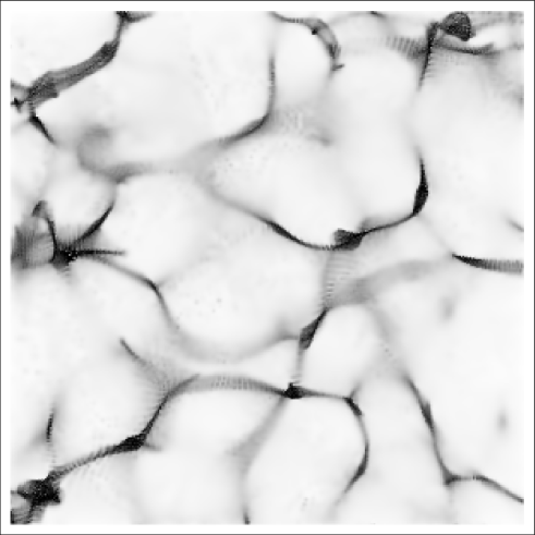
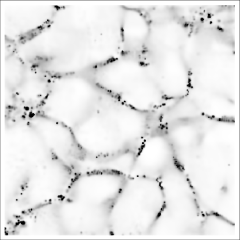
Thus, 2LPT positions and velocities can all be determined from the initial fluctuation field. In practice, we generate 2LPT positions and velocities using the algorithm described in detail in Appendix D of Scoccimarro (1998), where the Poisson equations are solved by standard fast Fourier transform methods. As mentioned before, 2LPT recovers the exact two and three-point statistics at large scales, and approximates very well higher-order ones (see e.g. Fig. 15 in Bouchet et al. 1995, and Table 2 in Scoccimarro 2000). It is possible to improve on 2LPT by going to third-order in the displacement field (3LPT), however it becomes more costly due to the need of solving three additional Poisson equations (Buchert 1994). 3LPT reproduces exactly up to four-point statistics, and improves the behavior in the underdense regions (where 2LPT tends to overestimate the density, see Bouchet et al. 1995).

Figure 1: A slice of 2LPT, 150 Mpc/h a side and 6 Mpc/h thick.

Figure 2: The same slice as previous figure for PTHalos.

3 From 2LPT to virialized haloes

The end result of 2LPT is a list of particle positions and velocities. These positions and velocities are not quite the same as those the particles would have had in a full $n$-body simulation which started from the same initial conditions. This section describes how to use our knowledge of fully nonlinear density and velocity fields to increase the agreement with simulations.

The primary difference between the 2LPT density field and that from a full $n$-body simulation of nonlinear gravitational clustering is that the 2LPT density field has no virialized objects. In a full simulation, however, most of the mass in a simulation box is partitioned into virialized haloes (e.g. Tormen 1998). For our purposes here, all virialized objects have well defined edges, and the edge, called the virial radius, is defined so that all virialized haloes have the same spherically averaged density, whatever their mass: $m\propto r_{\rm vir}^{3}$. Therefore, in what follows, we will make the simplifying assumption that all virialized haloes are spherical. (In fact, haloes have a range of shapes; allowing for a distribution of shapes is a detail which does not change the logic of our method, so we will comment on it in more detail later.)

We will approximate the effects of fully nonlinear clustering in two steps. First, we need a prescription for dividing up the 2LPT density field into a collection of virialized haloes. Once this has been done, we must decide how to distribute the mass associated with each halo around the halo centre-of-mass. This second step is more straightforward, so we will describe it first.

3.1 Virialized halo profiles

As noted above, we will assume that all dark matter haloes are spherically symmetric. High resolution $n$-body simulations (Navarro, Frenk & White 1997) show that the spherically averaged density run around the centre of a virialized halo containing mass $m$ within the virial radius $r_{\rm vir}$ is well fit by

$${\rho(r)\over\bar{\rho}}={\Delta_{\rm vir}(z)\over 3\Omega(z)}{c^{3}f(c)\over x(1+x)^{2}},\qquad{\rm where}\ x\equiv c(m)\,{r\over r_{\rm vir}},$$ (13)

where $\bar{\rho}(z)$ is the average density of the background universe at $z$, $\bar{\rho}(z)\,\Delta_{\rm vir}(z)/\Omega(z)$ is the average density within the virial radius ($\Delta_{\rm vir}\approx 178$ for all $z$ in an Einstein de-Sitter universe; it is $\approx 102$ at $z=0$ for the $\Lambda$CDM model we present results for in this paper), and $f(c)=[\ln(1+c)-c/(1+c)]^{-1}$. The density run is a broken power-law, with a shallower inner slope and a steeper outer slope. The exact shape of these two slopes is the subject of some debate. Although we will use the NFW form in what follows, it is trivial to modify our algorithm to generate profiles of the form given, e.g., by Hernquist (1990) or by Moore et al. (1999). The parameter $c$ is often called the central concentration of the halo. As NFW noted, more massive haloes are less centrally concentrated. We will use the parametrization of this trend provided by Bullock et al. (2001):

$$c(m)\approx{9\over(1+z)}\Big{(}\frac{m}{m_{*0}}\Big{)}^{-0.13},$$ (14)

where $m_{*0}$ is the standard non-linear mass scale (defined in the next subsection). Numerical simulations show that not all haloes of mass $m$ have the same density profile, there is considerable scatter. Fortunately, this scatter is well fit by using the same NFW shape for all haloes, but letting the concentration parameter have a Lognormal distribution with dispersion $\Delta(\log c)\approx 0.2$ (Jing 2000; Bullock et al. 2001). We include this scatter in PTHalos.

Equation (13) says that if the centre of mass of an $m$-halo is at position ${\bf x}$, then there will be $N_{\rm dm}\propto m$ particles distributed around ${\bf x}$ according to equation (13). This is easily done. For example, if the halo profile were an isothermal sphere ($\rho\propto r^{-2}$), then particle positions around the halo centre $(r,\theta,\phi)$ could be got by drawing random numbers distributed uniformly between zero and $r_{\rm vir}$ for the radial distance $r$ from the centre, uniform numbers between plus and minus one for $\cos\theta$, and uniform numbers between zero and two pi for $\phi$. Generating an NFW profile is only slightly more complicated.

Because the density run depends on halo mass $m$, the trick is to identify those positions in the 2LPT density field which should be identified with the centres-of-masses of $m$-haloes. The next subsection describes how to do this.

3.2 Halo masses and positions

Imagine comparing the 2LPT density and velocity fields with those from an $n$-body simulation which started from the same initial fluctuation field. One might imagine that the 2LPT density and velocity fields contain information about where bound objects in the $n$-body simulation formed. For example, perhaps the densest 2LPT regions are those regions which, in the $n$-body simulation, collapsed to form bound haloes. If so, then one might imagine running a friends-of-friends group finder on the 2LPT density field to identify these overdense regions. One could then use the number of particles associated with the friends-of-friends group as an estimate of the mass of the virialized halo which formed in the $n$-body simulation, and the position of the centre-of-mass of the group could be used as an estimate of the position of the corresponding halo. While such a procedure is possible in principle, running a group-finder can be quite time-consuming. This is the primary reason why we have adopted the approach we describe below.

At any given time, which we will label by redshift $z$, virialized haloes have a wide range of masses. Let $n(m|z)$ denote the comoving number density of haloes of mass $m$ at $z$. The shape of this universal mass function distribution is well approximated by

$${m^{2}\,n(m|z)\over\bar{\rho}}=\nu f(\nu)\,{{\rm d}{\rm ln}\nu\over{\rm d}{\rm ln}m},$$ (15)

where $\bar{\rho}$ denotes the comoving density of the background, and

$$\nu f(\nu)=2A\Big{(}1+(a\nu^{2})^{-p}\Big{)}\left(a\nu^{2}\over 2\pi\right)^{1/2}\,\exp\left(-{a\nu^{2}\over 2}\right).$$ (16)

Here $\nu\equiv\delta_{\rm sc}(z)/\sigma(m,z)$ where $\delta_{\rm sc}(z)$ is the collapse threshold given by the spherical collapse model (e.g. it is 1.68 in an Einstein-deSitter universe), $\sigma^{2}(m,z)$ is the linear theory variance in the density field when smoothed on the comoving scale $R=(3m/4\pi\bar{\rho})^{1/3}$ at $z$, and $A=0.5,0.322$, $p=0,0.3$ and $a=1,0.707$ for the mass functions given by Press & Schechter (1974) and Sheth & Tormen (1999), respectively. (Sheth, Mo & Tormen 2001 show that these two cases may be related to models in which objects form from spherical or ellipsoidal collapses, respectively. Jenkins et al. (2001) compare these mass functions with $n$-body simulations.) The number of haloes falls exponentially at large masses. Let $m_{*}$ denote the mass at which this cut-off sets in. Then $m_{*}$ is defined by requiring $\sigma(m_{*},z)\equiv\delta_{\rm sc}(z)$. The quantity $m_{*0}$ which should be used in equation (14) is got from setting $\sigma(m_{*0},0)\equiv\delta_{\rm sc}(0)$.

The distribution of haloes in dense regions is different from that in underdense regions: $n(m,\delta|z)\neq(1+\delta)\,n(m|z)$, where $\delta$ denotes the overdensity of the region. For example, the ratio of massive to less massive haloes is larger in dense regions than in underdense ones. A simple model for this dependence is

$$n(m,\delta|z)\approx\Bigl{[}1+b(m|z)\,\delta\Bigr{]}\,n(m|z),$$ (17)

where $\delta\equiv M/\bar{\rho}V-1$, and

$$b(m|z)=1+{a\nu^{2}-1\over\delta_{\rm sc}(z)}+{2p/\delta_{\rm sc}(z)\over 1+(a\nu^{2})^{p}}$$ (18)

(Mo & White 1996; Sheth & Tormen 1999). The actual detailed dependence of $n(m,\delta|z)$ on $\delta$ can be computed following Lemson & Kauffmann (1999), Sheth & Lemson (1999a) and Sheth & Tormen (2001), so we will not repeat the analysis here.

If we place a grid on the 2LPT density field, then some of the cells will be denser than others. We must find an algorithm which ensures that the distribution of halo masses in the different density cells follows the correct $n(m,\delta|z)$ relation.

We can do this as follows. The actual nonlinear density in $V$ at $z$ is given by $M/V\equiv\bar{\rho}(1+\delta)$. Let $\delta_{0}$ denote the value for the overdensity one would have predicted for such a region, had one used linear theory to make the prediction. Typically, we expect that if $\delta>0$, then $\delta_{0}<\delta$, and viceversa for underdense regions. A simple fitting formula to the relation between the nonlinear and the linear overdensities, $\delta$ and $\delta_{0}$, got from assuming that objects form from a spherical collapse in an Einstein-deSitter universe, has been provided by Mo & White (1996). We have checked that the following simple modification to their formula is accurate for all cosmologies of interest:

$$\delta_{0}\!\!\! = \!\!\!\left[1.68647-{1.35\over(1+\delta)^{2/3}}-{1.12431\over(1+\delta)^{1/2}}+{0.78785\over(1+\delta)^{0.58661}}\right]$$ (19)

$$\qquad\qquad\qquad\times\qquad{\delta_{\rm sc}(z)\over 1.68647}.$$

Now, what we are trying to do is to partition the mass $M$ in $V$ at $z$ up into subregions, each of nonlinear density $\Delta_{\rm vir}(z)\gg 1$, and hence each with predicted linear density $\delta_{\rm sc}(z)$.

This is extremely similar to what one does when one studies the merger histories of objects. Given the mass $M$ and the linear theory density $\delta_{0}$ associated with that mass, one studies the distribution of subclumps $m_{j}$ of $M$ at some earlier time when the critical density for collapse was $\delta_{\rm sc}(z)$. A number of merger history tree codes which do this are available. The algorithm described by Sheth & Lemson (1999b) is simple and efficient, so we will use it to partition the 2LPT mass $M$ up into virialized haloes. The only difference is that, whereas they were trying to generate the Press-Schechter mass function, we would like to generate the distribution which fits the simulations better. This can be done by making the following simple change to their algorithm.

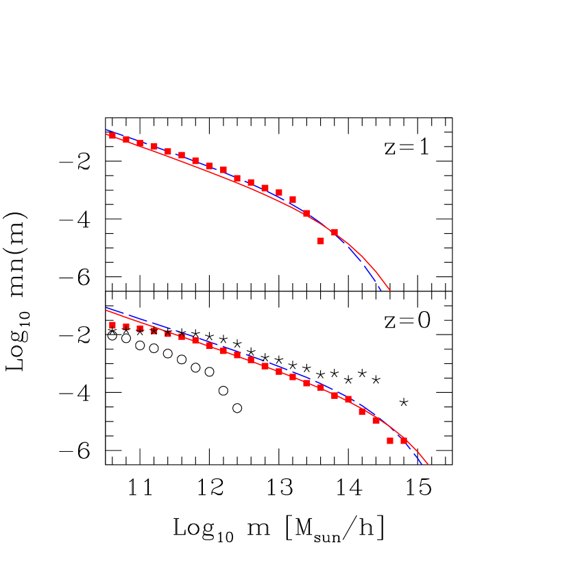
Sheth & Lemson’s algorithm loops over a range of ‘time’ steps, chooses a series of Gaussian random numbers $g_{i}$ at each time step, and then, for each $i$, makes use of $g_{i}^{-2}$. Their algorithm is fast because there are efficient ways to generate Gaussian variates. Therefore, if we modify the algorithm, we would like to do it in such a way that it still requires only Gaussian variates. For $\Lambda$CDM we have found that requiring the number of ‘time’ steps to equal ten, and then using $\ a\,[3+0.33/(1+|g_{i}|^{1.5})]/|g_{i}|$ instead of $g_{i}^{-2}$, where $a=0.707$ is the same parameter as in equation (16), is all that is required to generate a mass function which is more like the $n$-body simulations (see Fig. 3).

Figure 3: The halo mass function at $z=1$ (top) and $z=0$ (bottom). In each panel, squares show the output from PTHalos, solid line shows the fitting function which describes the $n$-body simulations, and dashed line shows the Press–Schechter mass function. Stars and circles in the bottom panel show the mass function in the densest and the least dense three percent of the box at $z=0$. These results correspond to flat $\Lambda$CDM realizations ($\sigma_{8}=0.9$, $\Omega_{m}=0.3$ at $z=0$) in a 100 Mpc/h box with mass resolution $m_{\rm min}=10^{10.5}M_{\sun}$/h and $R_{\rm grid}=12.5$ Mpc/h.

Notice that because $(1+\delta)\leq\Delta_{\rm vir}$, equation (19) guarantees that $\delta_{0}\leq\delta_{\rm sc}(z)$. Therefore, in essence, by using a merger tree code to perform the partition, we are making use of the following fact: a dense cell can be thought of as a region which will, at some point in the near future, become a virialized object. Therefore, when we view a dense cell at the present time, it is as though we are viewing a virialized object at a small ‘lookback time’ from the time it virialized. At small lookback times, most of the mass $M$ of an object is likely to be partitioned up into just a few pieces which are each a substantial fraction of $M$, because there has not been enough time for $M$ to have been split up into many smaller pieces. In hierarchical clustering models, the opposite is true at large lookback times. This provides a simple reason why the ratio of massive to less massive haloes is larger in dense regions than in underdense ones. In particular, this shows that when we partition the mass of a cell up as though we were partitioning the mass of a virialized halo up into subhaloes at high redshift, the only decision to be made is which redshift, which ‘lookback time’, to choose when running the merger tree algorithm. We have argued above that this choice depends on $\delta$: the exact transformation is given by equation (19).

To summarize, given the mass $M$ and the 2LPT overdensity $\delta$ in a cell $V$, a merger tree algorithm is used to split $M$ up into virialized haloes $m_{j}$. The next step is to decide where within $V$ to place the halo centres. We do this by assuming that the most massive haloes within $V$ occupy the densest subregion within $V$. Once this has been done, all that remains is to distribute particles around each halo centre as described in the previous subsection.

3.3 Nonlinear velocities

The final step is to account for the differences between the 2LPT and $n$-body velocity fields. In the $n$-body simulations, it is a good approximation to assume that the motion of a particle can be written as the sum of two terms:

$${\bf v}={\bf v}_{\rm vir}+{\bf v}_{\rm halo},$$ (20)

where the first term represents the virial motion of the particle within its parent halo, and the second term is the bulk motion of the halo as a whole (Sheth & Diaferio 2001). Furthermore, the virial motions within a halo are well approximated by velocities which are independent Gaussians in each of the three cartesian components, with rms values which depend on halo mass: $\sigma_{\rm vir}^{2}=\langle v_{\rm vir}^{2}\rangle\propto Gm/r_{\rm vir}\propto m^{2/3}$. In particular, we use (Bryan & Norman 1998; Sheth & Diaferio 2001)

$$\sigma_{\rm vir}=476f_{\rm vir}(\Delta_{nl}E(z)^{2})^{1/6}\Big{(}\frac{m}{10^{15}M_{\sun}/h}\Big{)}^{1/3}\ {\rm km/s},$$ (21)

where $f_{\rm vir}=0.9$ and $\Delta_{nl}=18\pi^{2}+60x-32x^{2}$ with $x=\Omega(z)-1$, $\Omega(z)=\Omega_{0}(1+z)^{3}/E(z)^{2}$, $E(z)^{2}=\Omega_{0}(1+z)^{3}+\Omega_{\Lambda}$ for a flat model with cosmological constant.

We assume that virial motions are uncorrelated with the direction or amplitude of ${\bf v}_{\rm halo}$. Therefore, if we substitute the 2LPT velocity vector at the position of the halo centre-of-mass for ${\bf v}_{\rm halo}$, and then add an uncorrelated vector of virial motions to each particle, and we do this for each of the particles in the halo, then the resulting velocity field should be quite similar to that in the $n$-body simulations. This is essentially a numerical implementation of the analytical model developed in Sheth et al (2001).

This is the final step in converting the 2LPT density and velocity fields to fields which resemble the $n$-body simulations more closely. The next section describes the algorithm which implements all of this.

4 PTHalos

4.1 The Algorithm

Given a realization of the large-scale density field, PTHalos assigns halo centers to appropriate 2LPT particles, and then generates NFW density profiles around them. This is done as follows.

• The desired mass resolution $m_{\rm min}$, the size of the simulation volume, and the cosmological model set the abundance of halos of mass larger than $m_{\rm min}$, $N_{\rm halos}$. Since halo centers are going to be identified as 2LPT particles, this sets the number of 2LPT particles to be used, $N_{\rm 2LPT}\approx N_{\rm halos}$, and thus their mass $m_{\rm 2LPT}$.

• The 2LPT box is divided into cubic cells of size $R_{\rm grid}$, and the mass in 2LPT particles $M_{i}$ in each cell $i$ is obtained. The choice of $R_{\rm grid}$ is dictated by the competing requirements that it be small enough so that the mass distribution is not rearranged at large scales (to preserve the correct correlations imposed by 2LPT), and large enough so that, within the cell, there can be halos sufficiently massive. Unless otherwise noted, we use $R_{\rm grid}=15$ Mpc/$h$. This corresponds roughly to a spherical cell of 8 Mpc/h radius which is the natural non-linear scale.

• Then, a merger history code is run on each cell $i$, which gives a partition of the cell mass $M_{i}$ into halos of smaller mass $m_{j}$ ($M_{i}=m_{1}+m_{2}+...$) down to the mass resolution.

• The 2LPT particles in a cell and the list of halos resulting from the merger history tree are matched so that most massive halos are centered about 2LPT particles in the densest regions. An exclusion volume of 2Mpc/$h$ (1Mpc/$h$ at $z=1$) radius is imposed about 2LPT centers in densities larger than 5.6 (set by the turnaround density in the spherical collapse model). Halos of mass $m_{j}$ are constructed about their 2LPT centers by sampling the NFW profile with the appropriate number of particles according to the mass resolution.

• Velocities are assigned using ${\bf v}={\bf v}_{\rm 2LPT}+{\bf v}_{\rm vir}$, where ${\bf v}_{\rm 2LPT}$ is the velocity of the 2LPT particle representing the halo center of mass, and ${\bf v}_{\rm vir}$ is a virial velocity drawn at random from a Maxwellian distribution with one-dimensional dispersion $\sigma_{\rm vir}(m_{j})$ given by Eq. 21. We require that the center of mass velocity of each halo equals that of the associated ${\bf v}_{\rm 2LPT}$; this is always possible because $N_{\rm 2LPT}\mathrel{\mathchoice{\lower 3.6pt\vbox{\halign{$\mathsurround=0pt\displaystyle\hfill#\hfil$\cr>\crcr\sim\crcr}}}{\lower 3.6pt\vbox{\halign{$\mathsurround=0pt\textstyle\hfill#\hfil$\cr>\crcr\sim\crcr}}}{\lower 3.6pt\vbox{\halign{$\mathsurround=0pt\scriptstyle\hfill#\hfil$\cr>\crcr\sim\crcr}}}{\lower 3.6pt\vbox{\halign{$\mathsurround=0pt\scriptscriptstyle\hfill#\hfil$\cr>\crcr\sim\crcr}}}}N_{\rm halos}$. This maintains the correct 2LPT correlations between density and velocity fields at large scales, which is important if we wish to have the correct large-scale redshift-space statistics.

• A galaxy distribution can be obtained by specifying how many galaxies, $N_{\rm gal}(m_{j})$ on average populate dark matter halos of mass $m_{j}$. Given this function, we use a binomial distribution (as explained in detail in Scoccimarro et al. 2001) to sample the NFW profile with the resulting number of galaxies. Benson et al. (2000) describe one possible alternative to the binomial. The binomial model we use has two free functions, the first and second moments of the number of galaxies per halo of mass $m$. The first moment is parametrized by a broken power-law with a low-mass cutoff, as described in Section 6; the second moment is related to the first taking into account that low-mass halos have a sub-Poisson dispersion (Kauffmann et al. 1999, Benson et al. 2000).

Fig. 1 shows a slice of 150 Mpc/$h$ a side and 6 Mpc/$h$ thick from a 2LPT distribution corresponding to $\Lambda$CDM with $\Omega_{m}=0.3$, $\Omega_{\Lambda}=0.7$, $\sigma_{8}=0.90$. Figure 2 shows the same slice in PTHalos, after 2LPT high-density regions have been replaced by virialized halos.

4.2 Memory Requirements and Speed

The PTHalos code requires a memory of 50 bytes per particle in the simulation box. Most importantly, a $300^{3}$ particle realization takes only about 5 minutes to generate on a single-CPU workstation, about $2-3$ orders of magnitude faster than $n$-body simulations. For particle numbers $N_{\rm par}\mathrel{\mathchoice{\lower 3.6pt\vbox{\halign{$\mathsurround=0pt\displaystyle\hfill#\hfil$\cr>\crcr\sim\crcr}}}{\lower 3.6pt\vbox{\halign{$\mathsurround=0pt\textstyle\hfill#\hfil$\cr>\crcr\sim\crcr}}}{\lower 3.6pt\vbox{\halign{$\mathsurround=0pt\scriptstyle\hfill#\hfil$\cr>\crcr\sim\crcr}}}{\lower 3.6pt\vbox{\halign{$\mathsurround=0pt\scriptscriptstyle\hfill#\hfil$\cr>\crcr\sim\crcr}}}}300^{3}$ approximately equal time is spent generating the 2LPT density field, imposing the spatial exclusion of massive halos, generating profiles and velocities, and writing the output files to disk. From tests we have performed up to $N_{\rm par}=400^{3}$, the run time scales roughly as $N_{\rm par}\ln(N_{\rm par})$.

Figure 4: The power spectrum as a function of scale for $\Lambda$CDM at $z=0$ (top) and $z=1$ (bottom). Symbols denote measurements in N-body simulations, solid lines correspond to PTHalos (averaged over 30 realizations), and dashed lines show linear perturbation theory.

Figure 5: The power spectrum in redshift-space at $z=0$ and $z=1$. The top panel shows the power spectrum monopole, the bottom panel corresponds to the quadrupole to monopole ratio. Line styles are as in Fig 4. The dotted line in the bottom panel shows the fitting formula by Hatton & Cole (1999).

Figure 6: The skewness ($S_{3}$) and kurtosis ($S_{4}$) as a function of smoothing scale $R$ in real (top) and redshift (bottom) space. Circles denote measurements in ten PTHalos realizations, and squares correspond to the average over four $n$-body simulations.

5 PTHalos vs. Numerical Simulations

We now turn to a quantitative comparison of clustering statistics for the dark matter obtained from PTHalos to $n$-body simulations. Application of PTHalos to the distribution of PSCz galaxies is discussed in Section 6.

5.1 Mass Function

A first test of our algorithm is to check that we obtain the correct mass function of dark matter halos. Fig. 3 shows the number density of haloes as a function of halo mass, for a simulation box of side 100 Mpc/h, mass resolution $m_{\rm min}=10^{10.5}M_{\sun}/h$ and $R_{\rm grid}=12.5$ Mpc/h. The symbols show the universal mass function one gets after using the merger tree algorithm to partition the 2LPT mass into haloes, and the solid curves show the fitting formula which describes the universal mass function in $n$-body simulations (equations 15 and 16). The symbols match the curves quite well, suggesting that our decision to use a merger tree algorithm was quite successful. The stars and circles in the $z=0$ panel show the mass function in the densest and the least dense three percent of the box. This shows that the densest cells contain the most massive haloes, as expected.

5.2 Power Spectrum in Real and Redshift Space

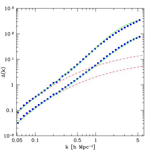
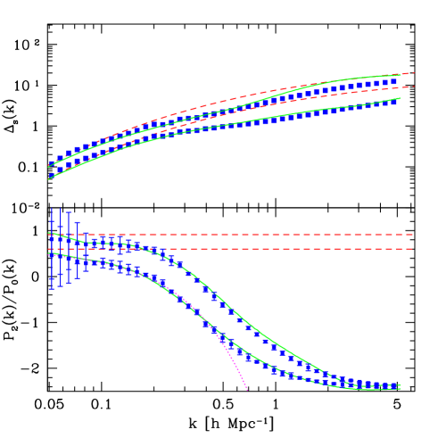
Figure 4 shows the power spectrum for the $\Lambda$CDM model at $z=0$ ($\sigma_{8}=0.90$, $\Omega_{m}=0.3$, $\Omega_{\Lambda}=0.7$) and $z=1$ ($\sigma_{8}=0.55$). The symbols in this and next figure denote the measurements in $n$-body simulations taken from Scoccimarro, Couchman & Frieman (1999a). The simulation was run by the Virgo Consortium; it corresponds to a single realization with $256^{3}$ particles in a 240 Mpc/h box. The dashed lines show the linear power spectrum, and the solid lines correspond to the measured power spectrum averaged over 30 PTHalos realizations. Figure 5 shows similar measurements for the power spectrum in redshift-space. The top panel corresponds to the monopole at $z=0$ (top) and $z=1$ (bottom) and the bottom panel shows the quadrupole to monopole ratio at $z=0$ (bottom) and $z=1$ (top). Error bars for the simulations correspond to the dispersion among four different lines of sight for the redshift-space mapping, done in the plane-parallel approximation, as assumed throughout this paper.

We see that the agreement between PTHalos and numerical simulations is very good, especially considering the simplicity of our algorithm. Similar results hold for the SCDM model. In redshift space, the power spectrum monopole is somewhat overestimated (for $z=0$) at small scales, suggesting perhaps our model for virial velocities is oversimplified (consistent with the analytic results presented in Sheth et al. 2001). Another possibility is inaccurate treatment of halo spatial exclusion effects; in redshift space halo-halo correlations are important down to smaller scales than in real space, because velocity dispersion suppresses halo profiles. We shall come back to this point in the next subsection when we study higher-order moments.

The excellent agreement shown for the quadrupole to monopole ratio even at scales below zero-crossing is very encouraging, since until now there was no alternative to numerical simulations that could provide an accurate treatment of redshift distortions. The problem, as emphasized by Hatton & Cole (1998) is that phenomenological models, where linear perturbation theory predictions (Kaiser 1987) are convolved with a kernel which describes the effects of velocity dispersion (Peacock & Dodds 1994, Park et al. 1994), tend to underestimate non-linear effects at large scales. Similarly, recent models of redshift distortions based on the halo model (White 2001, Seljak 2001) which assume linear perturbation theory for halo-halo correlations do not accurately reproduce the quadrupole moment, although they provide a good description of the power spectrum monopole (White 2001).

In our case the large-scale ($k\mathrel{\mathchoice{\lower 3.6pt\vbox{\halign{$\mathsurround=0pt\displaystyle\hfill#\hfil$\cr<\crcr\sim\crcr}}}{\lower 3.6pt\vbox{\halign{$\mathsurround=0pt\textstyle\hfill#\hfil$\cr<\crcr\sim\crcr}}}{\lower 3.6pt\vbox{\halign{$\mathsurround=0pt\scriptstyle\hfill#\hfil$\cr<\crcr\sim\crcr}}}{\lower 3.6pt\vbox{\halign{$\mathsurround=0pt\scriptscriptstyle\hfill#\hfil$\cr<\crcr\sim\crcr}}}}0.2$ h/Mpc) behavior of the monopole and quadrupole is dictated by 2LPT and has little to do with velocity dispersion (unlike in phenomenological models), and is reproduced very accurately. In fact, the bottom panel in Fig. 5 shows as dotted line the fitting formula found by Hatton & Cole (1999) empirically from an ensemble of $n$-body simulations. This relation, valid at scales larger than that of the quadrupole zero-crossing, fits our results extremely well. A detailed explanation of how perturbation theory can accurately describe the large-scale behavior of power spectrum multipoles will be presented elsewhere. Essentially, the large-scale pairwise velocity along the line of sight is strong enough to suppress the power spectrum monopole and drive the quadrupole to zero. The demonstration of this effect requires an accurate treatment of the non-linear nature of the redshift-space mapping (Scoccimarro et al. 1999a), which in our numerical treatment is trivially implemented since 2LPT treats the dynamics perturbatively but the mapping to redshift space is done exactly. Note that the deviations from linear perturbation theory are not negligible, even at scales larger than the non-linear scale $k\approx 0.2$ h/Mpc, in particular for the quadrupole.

5.3 Higher-Order Moments in Real and Redshift Space

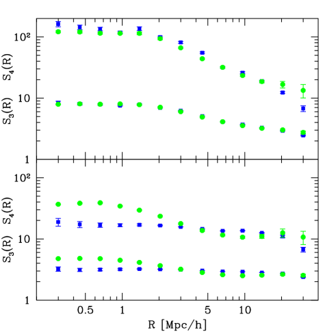
Figure 6 shows a comparison of PTHalos against $n$-body simulations for higher-order moments of the density field in real (top) and redshift (bottom) space. The figure shows the skewness $S_{3}(R)$ and kurtosis $S_{4}(R)$ as a function of smoothing scale $R$. Squares denote the average over 4 realizations of $\Lambda$CDM with $128^{3}$ particles in a box of $L_{\rm box}=300$ Mpc/h a side, obtained by running the Hydra code (Couchman et al. 1995). The circles denote the average of 10 realizations of PTHalos with $300^{3}$ particles in the same volume.

The agreement in real space is very good, particularly for the skewness. The runs in this figure were made using $R_{\rm grid}=20$ Mpc/h, we found that for $R_{\rm grid}=15$ Mpc/h, the skewness and kurtosis were underestimated at small scales $R<1$ Mpc/h by $10\%$ and $70\%$, respectively. Changing $R_{\rm grid}$ does not affect the power spectrum, but does affect increasingly more the higher-order moments which are most sensitive to the presence of high-mass halos. The choice of $R_{\rm grid}=15$ Mpc/h is thus a bit small for $L_{\rm box}=300$ Mpc/h, which leads to an underestimation of the number of very massive halos (which occasionally share more than one cell 15 Mpc/h a side).

In redshift space (bottom panel in Fig. 6) the situation is somewhat different, the small-scale skewness and kurtosis are actually higher in PTHalos than in $n$-body simulations. Increasing artificially the value of the velocity dispersion of halos, Eq. (21), does not fix the discrepancy (since the skewness and kurtosis are ratios of moments), suggesting perhaps that the problem is due to our approximate treatment of halo exclusion. More work is needed to fully understand the origin of this discrepancy.

5.4 Power Spectrum Covariance Matrix

As mentioned in the introduction, one of the motivations behind PTHalos is to provide a efficient tool for calculating accurate error bars and covariance matrices for clustering statistics including the effects of non-linear evolution, redshift distortions and galaxy biasing, that can be used to constrain cosmological parameters, galaxy formation models and the statistics of primordial fluctuations from analysis of clustering in upcoming galaxy surveys.

Here we consider what impact these effects have on the error bars and covariance matrix of the power spectrum. As it is well known, non-linear effects lead to increased error bars in individual band power estimates and introduce correlations between them that are absent in the Gaussian case (Meiksin & White 1999; Scoccimarro, Zaldarriaga & Hui 1999b; Hamilton 2000). In this Section we compare the predictions of PTHalos for the covariance matrix of the dark matter power spectrum against the numerical simulation results in Scoccimarro et al. (1999b), and present results that include redshift distortions and galaxy biasing as well.

All the covariance matrices are calculated using 300 realizations of PTHalos. The SCDM ($\Omega_{m}=1$, $\sigma_{8}=0.61$) realizations contain $200^{3}$ particles in a box of side $L_{\rm box}=100$ Mpc/h (identical volume and band power binning as the simulations we compare to, with bin width $\delta k=2\pi/100$ h/Mpc). The $\Lambda$CDM ($\Omega_{m}=0.3$, $\Omega_{\Lambda}=0.7$, $\sigma_{8}=0.9$) realizations contain $300^{3}$ particles in a box of side $L_{\rm box}=300$ Mpc/h. Finally, we construct realizations of galaxy distributions as described above with halo occupation numbers given by Eq. (22), derived in the next section from comparison to the PSCz survey. These have about $21.4\times 10^{6}$ galaxies in a box of side $L_{\rm box}=300$ Mpc/h (we do not include the survey selection function, our only purpose here is to explore the effects of galaxy weighing on the covariance matrix). In these cases, the width of bins in k-space is $\delta k=0.05$ h/Mpc

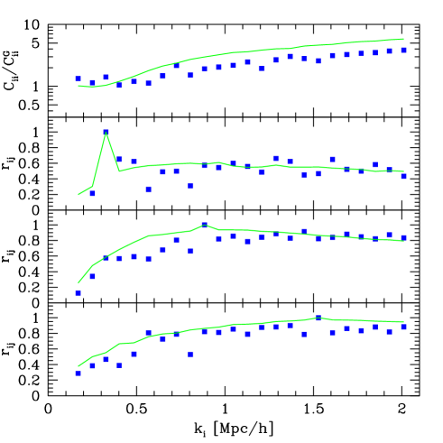
Figure 7 shows the results from PTHalos (solid lines) compared to the measurements obtained in Scoccimarro et al. (1999b) for the SCDM model. The top panel shows the ratio of the power spectrum errors (diagonal elements of the covariance matrix, $C_{ii}$) to those under the assumption of Gaussianity, $C_{ii}^{G}$. PTHalos seems to overestimate the errors at small scales by perhaps as much as $50\%$, although we regard this as a preliminary result since our $n$-body results contain only 20 realizations. Indeed, from our PTHalos Monte Carlo pool we see that error bars estimated from 20 realizations typically have a scatter of about $40\%$ compared to the results from 300 realizations. The remaining three panels in Fig. 7 show the cross-correlation coefficient, $r_{ij}\equiv C_{ij}/\sqrt{C_{ii}C_{jj}}$, between band powers centered at $k_{j}=0.32,0.88,1.52$ h/Mpc as a function $k_{i}$. Here the agreement seems much better, although it seems PTHalos slightly overestimates cross-correlations.

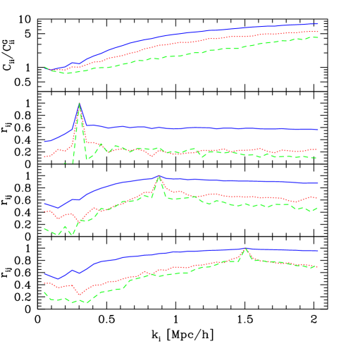
Figure 8 shows results in the same format as Fig. 7 but for $\Lambda$CDM PTHalos realizations for the dark matter power spectrum covariance matrix in real space (solid lines), redshift space (dotted lines), and for galaxies [with halo occupation numbers given by Eq. (22)] in redshift space (dashed lines). The effects of redshift distortions is to suppress the non-Gaussian contribution to the errors and the cross-correlations between band powers (Meiksin & White 1999; Scoccimarro et al. 1999b), due to the fact that velocity dispersion suppresses the higher-order moments, see Fig. 6. For galaxies, there is the additional effect of weighing the contribution of dark matter halos by the galaxy occupation number. At the scales shown here, this weighing suppresses non-Gaussianity and thus errors and cross-correlations. We find however that for $k\mathrel{\mathchoice{\lower 3.6pt\vbox{\halign{$\mathsurround=0pt\displaystyle\hfill#\hfil$\cr>\crcr\sim\crcr}}}{\lower 3.6pt\vbox{\halign{$\mathsurround=0pt\textstyle\hfill#\hfil$\cr>\crcr\sim\crcr}}}{\lower 3.6pt\vbox{\halign{$\mathsurround=0pt\scriptstyle\hfill#\hfil$\cr>\crcr\sim\crcr}}}{\lower 3.6pt\vbox{\halign{$\mathsurround=0pt\scriptscriptstyle\hfill#\hfil$\cr>\crcr\sim\crcr}}}}3$ h/Mpc (not shown), where the galaxy power spectrum is larger than the dark matter power spectrum, the situation reverses and galaxies have larger errors and cross-correlations than dark matter (as can be guessed e.g. from the asymptotic behavior in the top panel of Fig. 8).

Although galaxies in redshift space are generally less affected by non-Gaussianity, the effect is strong enough to be very important for constraining cosmological parameters from galaxy redshift surveys. Methods developed to decorrelate band powers (Hamilton 2000) were shown to work very well for the mass power spectrum when non-Gaussianities are modelled by the hierarchical model. It would be interesting to test these methods with PTHalos galaxy realizations to see how well they perform.

Another interesting application of our code would be to weak gravitational lensing, where studies have been made of error bars and covariance matrices for the power spectrum and moments of the convergence field (White & Hu 1999, Cooray & Hu 2000, Van Waerbeke et al 2001).

Figure 7: The Power Spectrum Covariance Matrix in SCDM $n$-body simulations (symbols) and PTHalos (solid lines). The top panel shows the ratio of the power spectrum errors to those under the assumption of Gaussianity. The remaining three panels show the cross-correlation coefficient $r_{ij}$ between band powers centered at $k_{j}=0.32,0.88,1.52$ h/Mpc as a function $k_{i}$ (Gaussianity corresponds to $r_{ij}=\delta_{ij}$).

Figure 8: Same as Fig. 7, but for $\Lambda$CDM PTHalos realizations. Solid lines denote the real space dark matter power spectrum covariance matrix, whereas dotted lines correspond to redshift space. Dashed lines show redshift-space measurements of galaxies given by Eq. (22).

6 Galaxy Distributions: Application to the PSCz survey

As discussed above, one the motivations behind PTHalos is to apply it to galaxy distributions, where its accuracy for galaxy clustering is expected to be comparable to standard methods which are computationally much more costly.

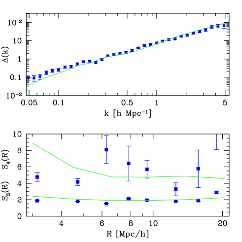
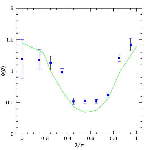
As a first example, we apply PTHalos to clustering in the PSCz survey (Saunders et al. 2000) assuming an underlying $\Lambda$CDM ($\Omega_{m}=0.3$, $\Omega_{\Lambda}=0.7$) cosmology. We use the following measurements of clustering statistics: the real-space power spectrum (Hamilton & Tegmark 2001) inverted from redshift-space, the skewness and kurtosis in redshift space as a function of scale (Szapudi et al. 2000) and the redshift-space bispectrum (Feldman et al. 2001).

In order to specify a galaxy distribution, we need to specify the moments of the number of galaxies $N_{\rm gal}$ per halo of mass $m$. We use a binomial distribution, as described in Scoccimarro et al. (2001), which has only 2 free functions, the first and second moments of $N_{\rm gal}(m)$. We relate these two by using the semianalytic model results of Kauffmann et al. (1999), where the dispersion in $N_{\rm gal}(m)$ is sub-Poisson for dark matter halos of mass $m<10^{13}M_{\sun}$/h, and Poisson otherwise. We then searched for a first moment parametrized by a broken power-law that leads to a good match with the real-space power spectrum of PSCz galaxies, and found

$$\mathop{\langle}N_{\rm gal}(m)\mathop{\rangle}=0.7\ (m/m_{0})^{\alpha},$$ (22)

where $\alpha=0$ for $8\times 10^{10}M_{\sun}/h\leq m\leq m_{0}$, $\alpha=0.7$ for $m>m_{0}$, $m_{0}=4\times 10^{11}M_{\sun}/h$. By definition, $N_{\rm gal}=0$ for masses below the mass resolution of the PTHalos realization, $8\times 10^{10}M_{\sun}/h$. The resulting power spectrum is shown in the top panel in Fig. 9 in solid lines, compared to the inferred power spectrum from the PSCz survey, shown in symbols with error bars (Hamilton & Tegmark 2001). Jing, Börner and Suto (2001) found recently that a similar relation, with $\alpha=0.75$, fits the two-point correlation function of PSCz galaxies.

We then calculated the skewness, kurtosis, and bispectrum in redshift-space (bottom panel in Fig. 9 and Fig. 10). The results turned out to be in very good agreement with the measurements in the PSCz survey (we only consider scales larger than $R=3$ Mpc/h in Fig. 9 given that PTHalos is not yet accurate enough for higher-order moments in redshift space, see Fig 6). This is very encouraging, because we did not attempt to fit them by adjusting the relation in equation (22). A similar result has been found by Szapudi et al. (2000) using the semianalytic models of Benson et al. (2000).

The resulting bias parameters are also in good agreement with the full likelihood analysis of the PSCz bispectrum (Feldman et al. 2001), $1/b_{1}\approx 1.2\pm 0.2$ and $b_{2}/b_{1}^{2}\approx-0.4\pm 0.2$. Indeed, from taking the ratio of the power spectrum of the PTHalos galaxies to the underlying dark matter spectrum at large scales, $k<0.3$ h/Mpc, we find $1/b_{1}=1.28$. Comparing the large-scale skewness for the dark matter, $S_{3}=2.6$, and for the PTHalos galaxies, $S_{3}^{\prime}=2$, and using $S_{3}^{\prime}\approx S_{3}/b_{1}+3b_{2}/b_{1}^{2}$ (Fry & Gaztañaga 1993), yields $b_{2}/b_{1}^{2}=-0.44$.

We stress that the result in Eq. (22) should not be considered a full analysis of constraints on galaxy occupation numbers from clustering of PSCz galaxies, since we have not explored the parameter space for $N_{\rm gal}(m)$ in a detailed fashion and only considered the constraint from the power spectrum measurements. However, the fact that this exercise led to very reasonable higher-order moments in redshift space gives us confidence that PTHalos can be successfully used to constrain galaxy formation models by using measurements of redshift-space clustering statistics at scales $R\mathrel{\mathchoice{\lower 3.6pt\vbox{\halign{$\mathsurround=0pt\displaystyle\hfill#\hfil$\cr>\crcr\sim\crcr}}}{\lower 3.6pt\vbox{\halign{$\mathsurround=0pt\textstyle\hfill#\hfil$\cr>\crcr\sim\crcr}}}{\lower 3.6pt\vbox{\halign{$\mathsurround=0pt\scriptstyle\hfill#\hfil$\cr>\crcr\sim\crcr}}}{\lower 3.6pt\vbox{\halign{$\mathsurround=0pt\scriptscriptstyle\hfill#\hfil$\cr>\crcr\sim\crcr}}}}3$ Mpc/h.

Figure 9: Top panel: real-space power spectrum inferred from the PSCz survey (Hamilton & Tegmark 2001) compared to the predictions for galaxies obeying the relation in Eq.(22). Bottom panel: same for the skewness $S_{3}$ and kurtosis $S_{4}$ (Szapudi et al 2000).

Figure 10: The redshift-space bispectrum in the weakly non-linear regime ($k<0.3$ h/Mpc) as a function of triangle shape for galaxies populating halos as in Eq.(22), compared to the PSCz bispectrum as measured by Feldman et al. (2001). The plot corresponds to wavectors in a ratio of approximately $k_{1}/k_{2}=0.5$ and angle between them equal to $\theta$. Error bars here represent the scatter in each bin from measurements of triangles of the same shape but somewhat different overall scale, and should only be considered a rough estimate of the uncertainties, see Feldman et al. (2001) for a full analysis.

7 Conclusions

We have described PTHalos, a fast algorithm which generates point distributions which have similar clustering statistics to those of the observed galaxy distribution. We have shown that our approach, although based on simple approximations, is able to reproduce the results of numerical simulations very well and requires minimal computational resources. Its speed and flexibility makes it suitable to explore parameter space in constraining cosmological parameters and galaxy formation models that can be later studied in more detail if necessary by perhaps more accurate (and computationally costly) methods.

As we noted in the introduction, although we only used PTHalos to model galaxy clustering, if one uses the PTHalos dark matter distribution in place of an $n$-body simulation, then, by placing a semianalytic galaxy formation package on top, one can model other properties of galaxies, such as luminosities and colours, as well. If one is interested in how bulge-to-disk ratios, or the correlation between galaxy luminosity and velocity dispersion, depend on local density, then the models described by, e.g., Dalcanton, Spergel & Summers (1997), Mo, Mao & White (1998), van den Bosch (2000), etc. can also be placed on top of the PTHalos dark matter distribution. These models may differ substantially in their formulation and in the specific physical processes which were considered relevant. The fact that PTHalos is several orders of magnitude faster than approaches which require the output of an $n$-body simulation means that it offers an efficient way of testing these different models.

There is an interesting history of making mock catalogs of the galaxy distribution in which one does not start with an $n$-body simulation. Soneira & Peebles (1978) describe an algorithm which generates point distributions which have the same small-scale two-point statistics as the observations. However, their method does not allow them to generate velocities and, because they were designed to work on small scales only, they do not include large-scale correlations. Motivated by the fact that the observed galaxy distribution is approximately Lognormal, Coles & Jones (1991) suggested that it might be a reasonable approximation to simply map initially Gaussian fluctuations to non-Gaussian ones by setting $\exp(\delta_{\rm init})=1+\delta_{\rm final}$. However, this mapping is only approximate, and it is not obvious how one might assign velocities, or account for the difference in clustering between the dark matter and galaxies. In addition, although it is possible to generate one-point higher-order moments by a local transformation of a Gaussian field, this does not generate the correct configuration dependence of multi-point correlation functions, which in gravitational instability are the result of the non-local character of Poisson’s equation.

Sheth & Saslaw (1994) described a halo-based algorithm which is similar in spirit to the one presented here. However, their prescription had no large-scale correlations (their haloes were given a Poisson spatial distribution), and they did not describe how to incorporate velocities into their model, nor how to allow for differences between the dark matter and the galaxy distributions. Bond & Myers (1996) described a halo-based algorithm which did include spatial correlations and used the Zel’dovich approximation for velocities. However, their algorithm was rather computationally intensive. Moreover, although it produced approximately the right number of massive halos, it was less accurate at the low mass end.

Our PTHalos algorithm represents a real improvement because:

• it has correct two- and three-point correlations on large-scales;

• it has accurate higher-order moments on all scales;

• it includes realistic velocity correlations; and

• it allows one to model the differences between the distributions of dark matter and different galaxy types—nontrivial biasing effects are rather simple to incorporate.

There are a number of inputs to PTHalos which are easily modified. For example, we distribute particles around halo centres so that they follow an NFW profile; this is easily changed to one’s favourite profile—a tophat, an isothermal sphere, or one of the profiles described by Hernquist (1990) or Moore et al. (1999). Also, our code assumes that all haloes are smooth, whereas haloes in simulations have substructure. Neglecting this fact is reasonable on all but the very smallest scales because substructure accounts for only about fifteen percent of the mass of a halo (e.g. Ghigna et al. 2000). In any case, Blasi & Sheth (2000) provide simple fitting formulae to Ghigna et al.’s simulations which make including substructure straightforward.

It is slightly more complicated to generate haloes with a range of ellipticities. There are, at present, no convenient parametrizations of the distribution of halo shapes in $n$-body simulations (see however Dubinski & Carlberg 1992). The ellipsoidal collapse model which reproduces the correct halo mass function makes specific predictions for this distribution (Sheth, Mo & Tormen 2001); in principle, it could be used to specify the distribution of shapes. The simplification of spherical halos leads to discrepancies in the bispectrum, at small scales the reduced bispectrum $Q$ looses the dependence on triangle shape at scales larger than those of the simulations (Scoccimarro et al. 2001). One the other hand, the numerical results in Ma & Fry (2000) suggest that except possibly for the smallest scales, the low-order spatial statistics at least are insensitive to whether or not the haloes are spherical.

Improvements which we hope to include in the near future include the following. One of the places in which PTHalos is not as accurate as we would like is in its assignment of virial velocities. At present, we assume that velocities within haloes are isotropic. Cole & Lacey (1996) show that this is not quite correct; haloes in simulations tend to have slightly more radial orbits near the edge of the halo. This is something we have included as a test but it turned out to be a small effect in the statistics we studied. However, in view of the deviations found for redshift-space higher-order moments, more work is needed to make sure our velocity statistics are accurate enough at small scales. In this connection, most importantly perhaps is that our present scheme which accounts for the fact that haloes may not overlap is somewhat adhoc. An improved treatment of exclusion, or a better algorithm for using the 2LPT density field to assign positions to the haloes output from the merger tree partition would be very useful. One promising option is to modify the approach described by Bond & Myers (1996), so that it can be applied to the 2LPT rather than the linear fluctuation field, to assign positions to the most massive halos. One could then use the merger tree algorithm to assign the mass which remains to less massive haloes—one of the advantages of Sheth & Lemson’s (1999b) merger tree algorithm is that it is easily adapted to construct partitions when it is known that some of the mass has already been assigned to more massive haloes.

To model deep galaxy redshift surveys, the angular correlations of galaxies, weak lensing observations, quasar absorption lines and the Ly-$\alpha$ forest, or the thermal and kinematic Sunyaev-Zel’dovich effects, rather than providing particle positions and velocities at a fixed epoch, it is more useful to have a simulation output particle positions and velocities along the observer’s light-cone. In PTHalos this is particularly straightforward, and is the subject of ongoing work.

Finally, another issue that is important for generating mock galaxy surveys is to adapt the simulation to the required survey geometry and selection function. At present we generate a cubical volume that encloses the survey volume and whose mean (constant) density matches the maximum density required by the survey in question, as usually done in mock catalogues constructed from $n$-body simulations (see e.g. Cole et al 1998 for a detailed exposition). This requires a lot more galaxies than really needed. The efficiency of PTHalos will be improved significantly by including these considerations from the start, rather than imposing them at the end. We hope to implement this in the next version of the code, which will become publically available.

8 acknowledgments

We thank Stephane Colombi, Lam Hui and Istvan Szapudi for useful discussions. RS thanks Fermilab, and RKS thanks NYU, for hospitality at the initial and final stages of this project. RKS is supported by the DOE and NASA grant NAG 5-7092 at Fermilab. The $n$-body simulations used in Figs. 6 and 7 were produced using the Hydra $n$-body code (Couchman, Thomas, & Pearce 1995). The $n$-body simulations used in Figs. 4-5 are publically available at http://www.mpa-garching.mpg.de/NumCos and were carried out at the Computer Center of the Max-Planck Society in Garching and at the EPCC in Edinburgh, as part of the Virgo Consortium project.

References

- [1] Benson A. J., Cole S., Frenk C. S., Baugh C. M., Lacey C. G., 2000, MNRAS, 311, 793
- [2] Benson A. J., Pearce F. R., Frenk C. S., Baugh C. M., Jenkins A., 2001, MNRAS, 320, 261
- [3] Blasi P., Sheth R. K., 2000, PLB, 486, 233
- [4] Bond J. R., Myers S. T., 1996, ApJS, 103, 1
- [5] Bryan, G. & Norman, M. 1998, ApJ, 495, 80
- [6] Bullock J. S., Kolatt T. S., Sigad Y., Somerville R. S., Kravtsov A. V., Klypin A. A., Primack J. R., Dekel A., 2001, MNRAS, 321, 559
- [7] Bouchet F. R., Colombi S., Hivon E., Juszkiewicz R., 1995, AA, 296, 575
- [8] Buchert T., Melott A. L., Wei A. G., 1994, AA, 288, 349
- [9] Buchert, T. 1996, MNRAS 267, 811
- [10] Cen, R. & Ostriker, J.P. 2000, ApJ, 538, 83
- [11] Cole S., Lacey C. G., 1996, MNRAS, 281, 716
- [12] Cole S., Hatton S., Weinbgerg D. H., Frenk C. S., 1998, MNRAS, 300, 945
- [13] Cole S., Lacey C. G., Baugh C. M., Frenk C. S., 2000, MNRAS, 319, 168
- [14] Coles P., Jones B., 1991, MNRAS, 248, 1
- [15] Connolly, A. et al., 2001, in preparation
- [16] Cooray, A., & Hu, W. 2000, astro-ph/0012087
- [17] Couchman H. M. P., Thomas P. A., Pearce F. R., 1995, ApJ, 452, 797
- [18] Dalcanton J. J., Spergel D. N., Summers F. J., 1997, ApJ, 482, 659
- [19] Dodelson, S. et al., 2001, in preparation
- [20] Dubinski, J. & Carlberg, R.G. 1992, ApJ, 378, 496
- [21] Feldman H. A., Frieman J. A., Fry J. N., Scoccimarro R., 2001, PRL, 86, 1434
- [22] Fry J. N., Gaztañaga E., 1993, ApJ, 413, 447
- [23] Ghigna S., Moore B., Governato F., Lake G., Quinn T., Stadel J., 2000, ApJ, 544, 616
- [24] Hamilton, A.J.S. 2000, MNRAS, 312, 257
- [25] Hamilton A. J. S., Tegmark M., 2001, MNRAS, submitted, astro-ph/0008392
- [26] Hatton, S. & Cole, S. 1998, MNRAS, 296, 10
- [27] Hatton, S. & Cole, S. 1999, MNRAS, 310, 1137
- [28] Hernquist L., 1990, ApJ, 356, 359
- [29] Jenkins A., Frenk C. S., White S. D. M., Colberg J. M., Cole S., Evrard A. E., Couchman H. M. P., Yoshida N., 2001, MNRAS, 321, 372
- [30] Jing Y. P., Mo H. J., Börner G., 1998, ApJ, 494, 1
- [31] Jing Y. P., 2000, ApJ, 535, 30
- [32] Jing Y. P., Börner G., Suto Y. 2001, astro-ph/0104023
- [33] Kaiser, N. 1987, MNRAS, 227, 1
- [34] Kauffmann G., Colberg J. M., Diaferio A., & White S. D. M., 1999, MNRAS, 303, 188
- [35] Lemson, G., Kauffmann G. 1999, MNRAS, 302, 111
- [36] Ma C-P., Fry J. N., 2000, ApJL, 531, 87
- [37] Meiksin, A.& White, M. 1999, MNRAS, 308, 1179
- [38] Mo H. J., Jing Y. P., Börner G., 1997, MNRAS, 286, 979
- [39] Mo H. J., White S. D. M., 1996, MNRAS, 282, 347
- [40] Mo H. J., Mao S., White S. D. M., 1998, MNRAS, 295, 319
- [41] Moore B., Quinn T., Governato F., Stadel J., Lake G., 1999, MNRAS, 310, 1147
- [42] Moutarde F., Alimi J.-M., Bouchet F. R., Pellat R., Ramani A., 1991, ApJ, 382, 377
- [43] Navarro J. F., Frenk C. S., White S. D. M., 1997, ApJ, 490, 493
- [44] Park, C., Vogeley, M.S., Geller, M., Huchra, J.P., ApJ, 431, 569
- [45] Peacock J. A., Dodds S. J., 1994, MNRAS, 267, 1020
- [46] Peacock J. A., Smith R. E., 2000, MNRAS, 318, 1144
- [47] Pearce F. P., Jenkins A., Frenk C. S., White S. D. M., Thomas P. A., Couchman H. M. P., Peacock J. A., Efstathiou G. (The Virgo Consortium) 2001, MNRAS, to appear, astro-ph/0010587
- [48] Press W., Schechter P., 1974, ApJ, 187, 425
- [49] Saunders, W., Sutherland, W.J., Maddox, S.J., Keeble, O., Oliver, S.J., Rowan-Robinson, M., McMahon, R.G., Efstathiou, G.P., Tadros, H., White, S.D.M., Frenk, C.S., Carramiñana, A., Hawkins, M.R.S. 2000, MNRAS, 317, 55
- [50] Scoccimarro R. 1998, MNRAS, 299, 1097
- [51] Scoccimarro, R., Couchman, H. & Frieman, J. 1999a, ApJ, 517, 531
- [52] Scoccimarro, R., Zaldarriaga, M. & Hui, L. 1999b, ApJ, 527, 1
- [53] Scoccimarro R. 2000, ApJ, 544, 597
- [54] Scoccimarro R., Sheth R. K., Hui L., Jain B., 2001, ApJ, 546, 20
- [55] Scranton R. et al., 2001, in preparation
- [56] Seljak, U., 2000, MNRAS, 318, 203
- [57] Seljak, U., 2001, MNRAS in press, astro-ph/0009016
- [58] Sheth R. K., Diaferio A., 2001, MNRAS, 322, 901
- [59] Sheth R. K., Hui, L., Diaferio A., & Scoccimarro, R., 2001, MNRAS, in press
- [60] Sheth R. K., Lemson G., 1999a, MNRAS, 304, 767
- [61] Sheth R. K., Lemson G., 1999b, MNRAS, 305, 946
- [62] Sheth R. K., Mo H. J., Tormen G., 2001, MNRAS, 323, 1
- [63] Sheth R. K., Saslaw W. C., 1994, ApJ, 437, 35
- [64] Sheth R. K., Tormen G., 1999, MNRAS, 308, 119
- [65] Sheth R. K., Tormen G. 2001, astro-ph/0105113
- [66] Somerville R. S.; Primack J. R., 1999, MNRAS, 310, 1087
- [67] Soneira R. M., Peebles P. J. E., 1978, AJ, 83, 845
- [68] Springel V., Yoshida N., White S. D. M., 2000, astro-ph/0003162.
- [69] Szalay, A. et al., 2001, in preparation
- [70] Szapudi I., Branchini E., Frenk C. S., Maddox S., Saunders W., 2000, MNRAS, 318, L45
- [71] Tegmark, M. et al., 2001, in preparation
- [72] Tormen, G. 1998, MNRAS, 297, 648
- [73] van den Bosch F. C., 2000, ApJ, 530, 177
- [74] Van Waerbeke, L., Hamana, T., Scoccimarro, R., Colombi, S., Bernardeau, F. 2001, MNRAS, 322, 918
- [75] White M. & Hu, W., 1999, ApJ, 537, 1
- [76] White, M. 2001, MNRAS, 321, 1
- [77] White S. D. M., Rees M. J., 1978, MNRAS, 183, 341
- [78] White S. D. M., Frenk C. S., 1991, ApJ, 379, 52
- [79] Zel’Dovich Y. B., 1970, AA, 5, 84