Non–Gaussian morphology on large scales:
Minkowski functionals of the REFLEX cluster catalogue

In order to quantify higher–order correlations of the galaxy cluster distribution we use a complete family of additive measures which give scale–dependent morphological information. Minkowski functionals can be expressed analytically in terms of integrals of $n$–point correlation functions. They can be compared with measured Minkowski functionals of volume limited samples extracted from the Reflex survey. We find significant non–Gaussian features in the large–scale spatial distribution of galaxy clusters. A Gauss–Poisson process can be excluded as a viable model for the distribution of galaxy clusters at the significance level of 95%.

1 Introduction

The spatial distribution of galaxy clusters poses important constraints on cosmological models. The abundance of clusters and especially its evolution with redshift is very sensitive to parameters of the cosmological models (see e.g. Kitayama & Suto 1997, Borgani et al. 1999, Bahcall 2000, Kerscher et al. 2001a). To quantify the large–scale structures traced by the galaxy clusters we have to go beyond the number density.

Scenarios describing the formation of structures in the Universe start with a mass density field showing only small deviations from the mean density. Inflationary scenarios suggest that these density fluctuations can be modeled as a Gaussian random field completely specified by its mean value and the power spectrum or two–point correlation function (e.g. Kolb & Turner 1990). In the initial stages of structure formation the linear approximation is often used to evolve these fluctuations preserving their Gaussian nature and increasing their amplitude only (see e.g. Peebles 1980). With growing over–density the nonlinear couplings become more and more important leading to a non–Gaussian density field. Also the process of galaxy formation may introduce non–Gaussian features if the “biasing” is non–linear (see e.g. Scoccimarro 2000). Typically one argues that on large scales, the evolution is still in the linear regime, and one expects that the smoothed density field is proportional to the initial Gaussian field. However, structures like walls and filaments were observed in the galaxy distribution on large scales (Huchra et al., 1990; Shectman et al., 1996). These non–Gaussian features appear at a low density contrast and are therefore hard to detect. The sensitivity of the Minkowski functionals, even if only a small number of points is available, allows us to quantify the non–Gaussian morphology of these structure on large scales. Walls and filaments were predicted by analytical and numerical work based on the Zel’dovich approximation (Zel’dovich, 1970; Arnol’d et al., 1982; Doroshkevich et al., 1996) and related approximations (Kofman et al., 1992; Bond et al., 1996). $N$–body simulations could verify that these structures are generic features of the gravitational collapse for Cold Dark Matter (CDM) like initial conditions (Melott & Shandarin, 1990; Jenkins et al., 1998).

Since observations supply us with the positions of galaxies and galaxy clusters in space, our methods will use this point distribution directly. No smoothing is involved. Therefore we have to give a clear definition what a “Gaussian” point distribution, the Gauss–Poisson process, is. Some of the statistical properties of random fields directly translate to similar statistical properties of point distributions, but also important differences show up. The equivalence of the Gauss–Poisson process with a simple Poisson cluster process, allows us to simulate a ‘Gaussian” point distribution (Kerscher, 2001). With these simulations we will perform a Monte–Carlo test to determine the significance of the non–Gaussian features in the cluster distribution.

Statistical measures provide important tools for the comparison of the large–scale structure in the Universe with theoretical models. The discriminative power of this comparison depends chiefly on the statistical measure. The most frequently employed measure was and still is the two–point correlation function, or the power spectrum. Both are nowadays an imperative in the analysis of any galaxy or cluster catalogue: for the Reflex cluster catalogue see Collins et al. (2000) and Schuecker et al. (2001). They give important information on the fluctuation spectrum of matter. However, they appear to be blind to morphological features. Indeed, completely different spatial patterns and point distributions could display the same two–point correlation function, i.e., no direct conclusions about the morphology of the structure can be drawn from an analysis with these two–point measures (Baddeley & Silverman, 1984; Szalay, 1997; Pan & Coles, 2000; Kerscher, 2001). Higher–order correlation functions immediately come to mind if one wants to go beyond the two–point correlation function. And indeed three–point correlations were detected in the distribution of galaxy clusters (Toth et al., 1989). However, there is a conceptual problem since $n$–point functions ($n\geq 3)$ depend on $3(n-1)-3$ parameters even for isotropic and homogeneous point distributions. Already for the three–point correlation function we are not aware of a study where its dependence on all three parameters was estimated. Clearly, integral information is mandatory and necessary. This may be accomplished e.g. for the three–point function by averaging over the shape of triangles, or by considering the (factorial) moments of counts in cells (see e.g. Peebles 1980 and Szapudi & Szalay 1993). Another effort to go beyond the two–point correlation function comprises the percolation analysis (Shandarin, 1983). Also the genus, closely related to the Euler characteristic, is often employed to quantify deviations from a Gaussian density fields (see e.g. Hamilton et al. 1986, Melott 1990 and references therein).

For the construction of statistical methods, sensitive to the large–scale structures, additivity is a heuristic principle which can guide us how to define useful measures which do not depend on all these parameters. Additivity yields robust, local decomposable measures. The mathematical discipline of integral geometry (see e.g. Hadwiger 1957) supplies us with a suitable family of such descriptors, known as Minkowski functionals. These measures embody information from every order of the correlation functions, are numerically robust even for small samples, and yield global as well as local morphological information. The Minkowski functionals are additive measures which allows us to calculate them efficiently by summing up their local contributions although they depend on all orders of correlation functions. The application of Minkowski functionals in statistical physics and cosmology are reviewed by Mecke (2000) and Kerscher (2000), respectively.

Samples of galaxy clusters are based mainly on optical observations, where the clusters are selected as galaxy over–densities in the two–dimensional maps on the celestial sphere (c.f. Abell 1958, Abell et al. 1989, Dalton et al. 1997, and Gal et al. 2000). Projection effects seem to have a non–negligible effect on the statistical analysis of these optically selected cluster samples (Katgert et al., 1996; van Haarlem et al., 1997). Only in recent years X–ray selected cluster samples have been completed. Since the X–ray luminosity is proportional to the baryonic density squared, over–densities are more emphasized. Consequently, the contamination of the catalogue by chance alignments due to projections is reduced (Böhringer et al., 2001). Assuming a virial relation, the X–ray luminosity of the galaxy cluster can be related to its mass.

2 Morphology of large scale structure

Minkowski functionals have been introduced to cosmology as a tool to quantify the morphology of large–scale structures by Mecke et al. (1994) where also a first analysis of the distribution of galaxy clusters based on the Abell et al. (1989) sample with a redshift compilation by Postman et al. (1992) was presented.

With Minkowski functionals we quantify the morphology of a sufficiently well behaved compact body $K\subset{\mathbb{R}}^{3}$ by assigning it a number $M_{\nu}(K)\in{\mathbb{R}}$. The Minkowski functionals are motion invariant

$$M_{\nu}(gK)=M_{\nu}(K),$$ (1)

where $g=({\mathbf{x}},\mathbf{\Theta})$ are the movements in three dimensions, i.e. translations ${\mathbf{x}}$ and rotations $\mathbf{\Theta}$. As already emphasized the additivity property

$$M_{\nu}(K\cup K^{\prime})=M_{\nu}(K)+M_{\nu}(K)-M_{\nu}(K\cap K^{\prime})$$ (2)

serves as the construction principle of these measures. All the Minkowski functionals have a straightforward interpretation in terms of geometrical and topological quantities as summarized in Table 1.

Table 1: Minkowski functionals $M_{\mu}$ and the normalized Minkowski functionals $\Phi_{\mu}$ (Eq. (8)) in three–dimensional space expressed in terms of more familiar geometric quantities.

geometric quantity		$\mu$	$M_{\mu}$	$\Phi_{\mu}$
volume	$V$	0	$V$	$V/(\tfrac{4\pi}{3}r^{3}N)$
surface area	$A$	1	$A/8$	$A/(4\pi r^{2}N)$
integral mean curvature	$H$	2	$H/(2\pi^{2})$	$H/(4\pi rN)$
Euler characteristic	$\chi$	3	$3\chi/(4\pi)$	$\chi/N$

Minkowski functionals are distinguished from other geometric measures by the theorem of Hadwiger (1957), which states that there are only four independent scalar functionals in three–dimensional space, which are motion invariant, additive, and continuous for convex bodies. Hence, every additive geometrical measure $M(K)$ which does not depend on the position and orientation of the body $K$ in three–dimensional space, can be written as a linear combination of the four Minkowski functionals:

$$M(K)=\sum_{\nu=0}^{3}c_{\nu}M_{\nu}(K).$$ (3)

Beisbart et al. (2001) discuss the vector valued extensions of the Minkowski functionals.

Figure 1: Dilated points: spheres of varying radius attached to the galaxy cluster from the Reflex sample L12 (see Table 2).

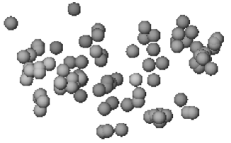
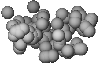
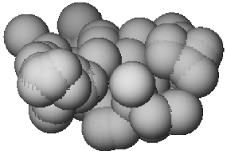
The cluster distribution provides us with a point set $X=\{{\mathbf{x}}_{i}\}_{i=1}^{N}$ in three–dimensional space. One may think of $X$ as a skeleton of the large–scale structures in the Universe. Since there are only four numbers of the MFs in three dimensions, compared to a correlation function, it is necessary to define morphological functions $M_{\mu}(r)$. The proper technique to do this for general random spatial structures are (erosion) dilation operations (see Fig. 1, and Serra 1982). In case of point patterns this techniques reduces to fixing balls $B_{r}$ of radius $r$ at each point. With Minkowski functionals we quantify the geometry and topology of union set of these balls ${\cal A}_{r}=\bigcup_{i=1}^{N}B_{r}({\mathbf{x}}_{i})$. The radius $r$ is employed as a diagnostic parameter. In such a way, we obtain scale–dependent integral information on higher–order correlations of the distribution of galaxy clusters and not only two–point correlation functions of the large–scale distribution. Erosion/dilation techniques combined with additive Minkowski functionals have been successfully applied in many areas, including condensed matter physics (Mecke, 2000), geology (Arns et al., 2001a, b), and digital image analysis (Serra, 1982, 1988).

2.1 The Boolean grain model

The simplest model of a random point distribution is the Poisson process. By attaching grains to each of the points, in our case balls of radius $r$, we arrive at the Boolean grain model. Mecke & Wagner (1991) presented a method to calculate mean volume densities of the Minkowski functionals for this model. We repeat their arguments, since its extension allows us to calculate the Minkowski functionals of correlated grains in Sect. 3.1.

Iterating the additivity relation (2) one obtains for the union ${\cal A}_{r}=\bigcup_{i=1}^{N}B_{r}({\mathbf{x}}_{i})$ of $N$ spheres $B_{i}=B_{r}({\mathbf{x}}_{i})$ of radius $r$ and center ${\mathbf{x}}_{i}$ the inclusion–exclusion formula

$$M_{\nu}({\cal A}_{r})=\sum_{i}M_{\nu}(B_{i})-\sum_{i<j}M_{\nu}(B_{i}\cap B_{j})+\\ +\ldots(-1)^{N+1}M_{\nu}(B_{1}\cap\ldots\cap B_{N})\;.$$ (4)

Generally, a point process in a domain $\Omega$ with volume $|\Omega|$ is specified by a sequence of product densities $\varrho_{n}({\mathbf{x}}_{1},\ldots,{\mathbf{x}}_{n})$ with the mean number density $\varrho\equiv\varrho_{1}({\mathbf{x}}_{1})$. $\varrho_{n}({\mathbf{x}}_{1},\ldots,{\mathbf{x}}_{n}){\rm d}V_{1}\ldots{\rm d}V_{n}$ is the probability of finding $n$ points in the volume elements ${\rm d}V_{1}$ to ${\rm d}V_{n}$. The volume density ${m}_{\nu}({\cal A}_{r})$ of the $\nu$–th Minkowski functional per unit volume for the augmented coverage ${\cal A}_{r}$ are then obtained from the inclusion–exclusion formula (4) in the form

$${m}_{\nu}\big{(}{\cal A}_{r};\{\varrho_{n}\}\big{)}=\\ \sum_{n=1}^{\infty}\frac{(-1)^{n+1}}{n!|\Omega|}\int\limits_{\Omega}{\rm d}\Gamma_{n}\ M_{\nu}\Bigg{(}\bigcap_{i=1}^{n}B_{r}({\mathbf{x}}_{i})\Bigg{)}\ \varrho_{n}(\Gamma_{n})$$ (5)

where we introduced, for convenience, the variable $\Gamma_{n}=({\mathbf{x}}_{1},\ldots,{\mathbf{x}}_{n})$ with the integration measure $\int_{\Omega}d\Gamma_{n}=\prod_{i=1}^{n}\int_{\Omega}d{\mathbf{x}}_{i}$. Obviously, the Minkowski functionals embody information from every order $n$ of the $n$–point densities $\varrho_{n}({\mathbf{x}}_{1},\ldots,{\mathbf{x}}_{n})$. If the product densities $\varrho_{n}({\mathbf{x}}_{1},\ldots,{\mathbf{x}}_{n})=\varrho^{n}$ were independent of position (Poisson distribution of density $\varrho=N/|\Omega|$), the integrals in Eq. (5) can be performed using the fundamental kinematic formula (Blaschke 1936, Santaló 1976)

$$\int\limits_{\cal G}{\rm d}g\ M_{\nu}(K\cap gK^{\prime})=\sum_{\mu=0}^{\nu}\binom{\nu}{\mu}M_{\mu}(K)M_{\nu-\mu}(K^{\prime}).$$ (6)

Equation (6) describes the factorization of the Minkowski functionals of the intersection $K\cap K^{\prime}$ of two bodies $K$ and $K^{\prime}$ if one integrates over the motions $g=({\mathbf{x}},\mathbf{\Theta})$, i.e. translations ${\mathbf{x}}$ and rotations $\mathbf{\Theta}$ of $K^{\prime}$. For Poisson distributed spheres $B_{r}$ of radius $r$ one obtains the mean values of the Minkowski functionals per unit volume (Mecke & Wagner 1991, Stoyan et al. 1995)

$${m}_{\nu}({\cal A}_{r};\varrho)=\frac{\partial^{\nu}}{\partial t^{\nu}}\Bigg{\{}1-\exp\Bigg{[}-\varrho\sum\limits_{\mu=0}^{d}\frac{t^{\mu}}{\mu!}M_{\mu}(B_{r})\Bigg{]}\Bigg{\}}\Bigg{|}_{t=0}$$ (7)

and particularly in three dimensions the normalized Minkowski functionals

$$\Phi_{\nu}(r)=\frac{{m}_{\nu}({\cal A}_{r})}{M_{\nu}(B_{r})\;\varrho}$$ (8)

read with $\eta=\frac{4\pi}{3}r^{3}\varrho$:

$$\begin{array}[]{ll}\Phi_{0}(r;\varrho)=&(1-{\rm e}^{-\eta})/\eta\;\;,\\ \Phi_{1}(r;\varrho)=&{\rm e}^{-\eta}\;\;,\\ \Phi_{2}(r;\varrho)=&(1-\frac{3\pi^{2}}{32}\eta){\rm e}^{-\eta}\;\;,\\ \Phi_{3}(r;\varrho)=&(1-3\eta+\frac{3\pi^{2}}{32}\eta^{2}){\rm e}^{-\eta}\;\;.\\ \end{array}$$ (9)

2.2 The Reflex cluster sample

The construction of the Reflex cluster sample is described in detail by Böhringer et al. (2001) and the statistics of the cluster distribution is described by Collins et al. (2000) for the two-point correlation function and in Schuecker et al. (2001) for the density fluctuation power spectrum. The survey area covers the southern sky up to the declination $\delta\leq 2.5^{o}$ avoiding the band of the Milky Way, $|b_{II}|\leq 20^{o}$ and the regions of the Magellanic clouds. The total survey area is 13924 $\deg^{2}$ or 4.24 ster. Tests including the number counts ($\log{N}\log{S}$–function), the comoving densities, $\langle V/V_{max}\rangle$ tests, and comparisons to simulations, described in the above mentioned papers, show that the selection function is well documented.

The X–ray detection of the clusters is based on the second processing of the RASS (ROSAT All Sky Survey, Voges et al. 1999) exploiting a primary (MPE internal) source detection list comprising 54076 sources in the Reflex area down to a detection likelihood of $L\geq 7$ (see Voges et al. 1999). For all these sources the X–ray parameters are reanalysed by the growth curve analysis method as described by Böhringer et al. (2000) which provides a flux measurement with significantly less discrimination against extended X–ray sources than provided by the standard analysis of the RASS. The results of this reanalysis are used to produce a flux–limited sample of RASS sources with a nominal flux $F_{x}\geq 3\cdot 10^{-12}$ erg s^-1 cm^-2 in the energy band (0.1–2.4 keV).

The cluster candidates are finally identified or removed from the sample as non–cluster sources by a detailed documentation of the X–ray and optical source properties, literature information, and spectroscopic information including redshift measurements obtained by follow–up observations within the frame of an ESO key program. Further tests of the sample completeness based on a search for clusters among the significantly extended X–ray sources and a search for X–ray emission from clusters cataloged by Abell et al. (1989) independent of the RASS source detection supports the completeness estimate of $>90\%$ for a flux–limit of $3\cdot 10^{-12}\text{erg}\text{s}^{-1}\text{cm}^{-2}$. The high completeness concerning the optical identification makes the data set an effectively X–ray selected sample of galaxy clusters. The final cluster sample includes 452 clusters and there are three objects left in the list with uncertain identifications and redshifts. These three objects are excluded here in the further analysis.

Figure 2: Luminosity – redshift distribution of Reflex clusters of galaxies (points) and the applied ranges for the extraction of volume–limited subsamples. The redshift and luminosity intervals of the respective volume–limited subsamples L05, L12, L20, and L30 are marked by continuous, short–dashed, long–dashed, and dotted lines. The subsamples are described in Table 2. Note that for conventional reasons the X–ray luminosities are given in units of $H_{0}=50\,{\rm km}\,{\rm s}^{-1}\,{\rm Mpc}^{-1}$.

For the determination of MFs complete volume–limited subsamples are needed. The Reflex cluster sample is per construction X–ray flux–limited so that the fraction of luminous clusters increases with redshift (see Fig. 2). Volume–limited distributions are selected by introducing upper redshift and lower luminosity limits (vertical and horizontal lines in Fig. 2). In order to reduce possible (error migration) effects which might occur at the flux–limit (e.g., Eddington 1940) the upper redshift limits are set slightly below the formal redshift limit, especially for large luminosities where the effects could be largest.

The completeness of the different volume–limited subsamples is illustrated in Fig. 3 in Schuecker et al. (2001) which includes the subsamples denoted by L05 to L30 in Table 2. Similar volume–limited samples as listed in Table 2 have been used by Collins et al. (2000) in their analysis using the two–point correlation function. Comoving distances have been calculated according to the Mattig formula with $\Omega=1$, $h=0.5$, and $\Lambda=0$. The flat redshift–independent distribution of comoving cluster number density suggests the absence of large incompleteness effects of the subsamples in the redshift range $0\leq{z}\leq 0.15$. We thus expect no significant artificial fluctuations introduced by incompleteness effects on scales up to comoving radial distances of $R<400\,h^{-1}\,{\rm Mpc}$.

Table 2: The volume–limited cluster samples used in our investigations consisting out of $N$ clusters closer than $R$ with X–ray luminosity higher than $L_{\rm min}$. The constraint $\varrho C_{2}$ will be explained in Sect. 4.

Sample	$R$	$L_{\rm min}$	N	$\varrho$	$\varrho C_{2}$
	[Mpc/h]	[erg/s]		[$h^{3}\text{Mpc}^{-3}$]
L05	180	$0.5\times 10^{44}$	74	$8.9\times 10^{-6}$	3.2
L12	260	$1.2\times 10^{44}$	95	$3.8\times 10^{-6}$	2.2
L20	330	$2.0\times 10^{44}$	86	$1.7\times 10^{-6}$	0.6
L30	385	$3.0\times 10^{44}$	62	$0.8\times 10^{-6}$	0.3

2.3 Minkowski functionals of the Reflex clusters

To study the morphology of the large–scale distribution of galaxy clusters we consider a series of volume–limited samples from the Reflex cluster catalogue (Böhringer et al., 2001). The volume densities ${m}_{\mu}$ of the Minkowski functionals were calculated using the minus–sampling boundary correction, based on partial Minkowski functionals as suggested by Mecke et al. (1994) (for details see Schmalzing & Diaferio 2000). The survey is bounded by $\delta<2.5^{\circ}$ and $|b|>20^{\circ}$, but also several regions in the small and large Magelanic clouds were excluded from the sample (for details see Böhringer et al. 2001). To estimate their influence on the Minkowski functionals of the samples we filled these regions with random points with the same number density. The comparison in Figs. 3–6 shows nearly identical results for filled or unfilled regions in the Magelanic clouds.

Figure 3: Minkowski functionals of the volume–limited sample L05 (solid line) compared to the Minkowski functionals of a Poisson process with the same number density (dotted line, gray shaded one–$\sigma$ area). The numerically determined mean is in perfect accordance with Eq. (9). The dashed one–$\sigma$ area is obtained by filling the excluded area around the small and large Magelanic clouds with randomly distributed points of the same number density as the rest of the sample.

Figure 4: Minkowski functionals of the volume–limited sample L12. Same conventions as in Fig. 3.

Figure 5: Minkowski functionals of the volume–limited sample L20. Same conventions as in Fig. 3.

Figure 6: Minkowski functionals of the volume–limited sample L30. Same conventions as in Fig. 3.

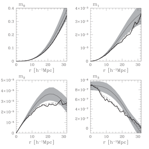
The overall features seen in the Minkowski functionals of the Reflex clusters are similar to the one observed in the Abell/ACO cluster sample of Plionis & Valdarnini (1991) as analyzed by Kerscher et al. (1997). We are limited by the smaller sample size and the boundary correction used. Only few galaxy clusters contribute to the Minkowski functionals for large radii. Therefore we are not able to trace the large–scale structure to the limit where the sample volume is filled by the union set of balls. Additionally to the Minkowski functionals of the clusters the results for a Poisson process with the same number density inside the sample geometry is shown in the Figs. 3–6. Increasing the depth of the volume–limited samples from L05 to L30 the Minkowski functionals show a clear trend from strong clustering towards only small differences from the Poisson distribution. Increasing the depth of the volume–limited samples we allow for clusters with higher X–ray luminosity. Considering the amplitude of the two–point correlation function, galaxy clusters with higher X–ray luminosity should show stronger correlations (Kaiser, 1984; Bardeen et al., 1986). However, in the deeper volume–limited samples, with the more luminous clusters, also the number density decreases. The sparseness of the point distribution competes with the increased amplitude of the two–point correlation function. Indeed, for quite general conditions, a point distribution converges towards a Poisson process under thinning, i.e. under randomly deleting points (e.g. Daley & Vere-Jones 1988, Sect. 9.3). For the Minkowski functionals the behavior in sparse samples may be explained by considering the expansion of the normalized Minkowski functionals $\Phi_{\mu}$ in terms of $\eta=\varrho(4\pi/3)r^{3}$ around zero (see also Kerscher et al. 2001b). Based on the expansion (5) of MFs in terms of $n$–point densities one gets to the lowest order in $\eta$

$$\Phi_{\mu}({\cal A}_{r})=\\ 1-\eta\ \frac{3}{2r^{3}}\int_{0}^{2r}{\rm d}s\ s^{2}\ I_{\mu}(r;s)\Big{(}1+\xi_{2}(s)\Big{)}+O(\eta^{2})\;.$$ (10)

The functions

$$\begin{array}[]{rl}I_{0}(r;s)=&1-\frac{3}{2}\frac{s}{2r}+\frac{1}{2}\big{(}\frac{s}{2r}\big{)}^{3},\\ I_{1}(r;s)=&1-\frac{s}{2r},\\ I_{2}(r;s)=&1-\frac{s}{2r}+\big{(}\frac{\pi}{4}-\frac{1}{2}\arccos\frac{s}{2r}\big{)}\Big{(}1-\big{(}\frac{s}{2r}\big{)}^{2}\Big{)}^{\frac{1}{2}},\\ I_{3}(r;s)=&\Theta(2r-s)\\ \end{array}$$ (11)

resemble the Minkowski functionals $I_{\nu}(r;|{\mathbf{x}}|)=M_{\mu}(B_{r}(\mathbf{0})\cap B_{r}({\mathbf{x}}))/M_{\mu}(B_{r})$ of the intersection of two spheres of radius $r$ and distance $|{\mathbf{x}}|$. $\Theta(q)$ is the step function equal zero for $q<0$ and one for $q>0$. In Eq. (10) the integral and its pre–factor give a dimensionless geometric number depending on the correlation function $\xi_{2}(s)$ and the measure $M_{\mu}$. Terms proportional to $\eta^{n}$ include intersections of $n$ spheres weighted by the $n$–point densities. Only the two–point correlation function is important for small $\eta$, but the Minkowski functionals become increasingly more sensitive to higher–order correlations with larger $\eta$. For very small $\eta$ we essentially arrive at a Poisson process as numerically verified by Kerscher et al. (1998). A small $\eta$ may be obtained either with a small radius $r$ of the spheres, or, as in our case, by a low number density $\varrho$.

Now let us describe the features in the MFs in more detail. The strong clumping in the distribution of galaxy clusters is causing the lowered values of the volume densities $m_{\mu}$ of the Minkowski functionals compared to the Poisson values. In a clustered point distribution, the spheres in the union set ${\cal A}_{r}=\bigcup_{i=1}^{N}B_{r}({\mathbf{x}}_{i})$ overlap significantly already for small radii. This is leading to a reduced density of the volume $m_{0}$, surface area $m_{1}$, and integral mean curvature $m_{2}$. The density of the Euler characteristic $m_{3}$ decreases since for small radii mainly the number of connected objects is counted – no tunnels and cavities have formed yet. A tunnel through the body ${\cal A}_{r}$ gives a negative contribution of minus one to the Euler characteristic. In the sample L20 we observe the zero crossing of the Euler characteristic indicating that an interconnected network of tunnels, a sponge–like, bi–continuous “cosmic web” has formed for radii around 35$h^{-1}$Mpc.

In the deeper samples L20 and L30 the volume density $m_{0}$ shows a tendency towards increased values compared to a Poisson process. With our estimator for the MFs, we successively shrink the sample proportional to $r$, where $r$ is the radius of the spheres $B_{r}$. Therefore, we mainly probe the central region of the sample for large $r$. The increased $m_{0}$ is caused by gradients in the number density $\varrho$ of the Reflex cluster sample, specifically the local under–density of clusters out to approximately 100$h^{-1}$Mpc (see Schuecker et al. 2001, and for galaxies Zucca et al. 1997).

There is no easy relation between the scale $s$ of fluctuations in the number density as probed by $\xi_{2}(s)$ and the radius $r$ of the spheres used in the MF analysis. As can be seen from Eqs. (5) and (15) weighted integrals over all scales contribute to the MFs at a given radius $r$. However, with the radius $r$ of the spheres $B_{r}$ we probe the geometry and topology of the cluster distribution in a scale–dependent way. The radius $r$ can be regarded as a geometrical scale, e.g. the radius $r_{p}$ of the first zero of the Euler characteristic $m_{3}({\cal A}_{r_{p}})=0$ is an estimate of the percolation threshold for our system of mono–disperse spheres (Mecke & Wagner, 1991). At this scale $r_{p}$ the large–scale structure elements (walls, filaments, clusters) form a percolating network.

3 Higher–order correlations in point distribution

3.1 Minkowski functionals for correlated grains

As for the Poisson process (Mecke & Wagner 1991, and Sect. 2.1) one may calculate the Minkowski functionals of correlated grains, in our case spheres centered on a clustered point set (Mecke 1994, Schmalzing et al. 1999, Mecke 2000). Our main analytic result Eqs. (15) and (16) expresses the Minkowski functions $M_{\nu}(r)$ in terms of centered correlation functions which allows a direct comparison of measured functions with a Gaussian model where higher correlations are set to zero.

The expression (5) may be used to calculate the Minkowski functionals for correlated grains given the $n$–point densities $\varrho_{n}({\mathbf{x}}_{1},\ldots,{\mathbf{x}}_{n})$ of the point distribution. An alternative and sometimes more convenient expression for the densities ${m}_{\nu}({\cal A}_{r})$ than Eq. (5) can be obtained in terms of the cumulants, the connected or centered correlation functions $\xi_{n}(\Gamma_{n})$ with $\xi_{1}({\mathbf{x}}_{1})=1$. For the two–point correlation function we have

$$\xi_{2}(r)+1=\xi_{2}({\mathbf{x}}_{1},{\mathbf{x}}_{2})+1=\frac{\varrho_{2}({\mathbf{x}}_{1},{\mathbf{x}}_{2})}{\varrho^{2}},$$ (12)

with $r=|{\mathbf{x}}_{2}-{\mathbf{x}}_{1}|$, and in general

$$\varrho_{n}(\Gamma_{n})=\varrho^{n}\sum_{\{{\cal P}\}}\prod_{i=1}^{|{\cal P}|}\xi_{p_{i}}(\Gamma_{p_{i}})$$ (13)

Thus, the product densities $\varrho_{n}$ of order $n$ is given by a sum over all possible partitions ${\cal P}$ of the coordinates $\Gamma_{n}=({\mathbf{x}}_{1},\ldots,{\mathbf{x}}_{n})$ into $|{\cal P}|$ parts of $p_{i}$ elements. Each vector ${\mathbf{x}}_{j}\in\Gamma_{n}$ occurs exactly once as an argument ${\mathbf{x}}_{j}\in\Gamma_{p_{i}}$ of a cumulant $\xi_{p_{i}}(\Gamma_{p_{i}})$ on the right side, i.e., $\sum_{i=1}^{|{\cal P}|}p_{i}=n$.

Using the additivity relation (2) and the kinematic formula (6) of the Minkowski functionals one can follow the derivation in Mecke & Wagner (1991) so that one immediately obtains the expression for the intensities (Mecke, 1994)

$${m}_{\nu}\big{(}{\cal A}_{r};\{\xi_{n}\}\big{)}=\\ \frac{\partial^{\nu}}{\partial t^{\nu}}\Bigg{\{}1-\exp\bigg{[}-\varrho\sum\limits_{\mu=0}^{d}\frac{t^{\mu}}{\mu!}{\overline{M}}_{\mu}(r;\varrho,\{\xi_{n}\})M_{\mu}(B_{r})\bigg{]}\Bigg{\}}\Bigg{|}_{t=0}$$ (14)

due to the factorization of the integral in Eq. (5) (compare with Eq. (7)). The normalized specific Minkowski functionals

$${\overline{M}}_{\nu}(r;\varrho,\{\xi_{n}\})=\sum_{n=1}^{\infty}\frac{(-\varrho)^{n-1}}{n!}\times\\ \times\int\limits_{\Omega}{\rm d}\Gamma_{n}\ \frac{M_{\nu}\big{(}\bigcap_{i=1}^{n}B_{r}({\mathbf{x}}_{i})\big{)}}{M_{\nu}(B_{r})|\Omega|}\ \xi_{n}({\mathbf{x}}_{1},\ldots,{\mathbf{x}}_{n})$$ (15)

describe the deviation from a Poisson process (compare Eq. (7)). For Poisson distributed spheres with vanishing cumulants $\xi_{n}(\Gamma_{n})=0$ one recovers ${\overline{M}}_{\nu}=1$. The specific Minkowski functionals depend on the radius $r$, the product density $\varrho$, and all of the correlation functions $\xi_{n}({\mathbf{x}}_{1},\ldots,{\mathbf{x}}_{n})$. In particular, one obtains for the normalized Minkowski functionals in three dimensions ($\eta=\frac{4\pi}{3}r^{3}\varrho$)

$$\begin{array}[]{l}\Phi_{0}(r;\varrho,\{\xi_{n}\})=\Big{(}1-{\rm e}^{-\eta{\overline{M}}_{0}}\Big{)}/\eta\\ \Phi_{1}(r;\varrho,\{\xi_{n}\})={\overline{M}}_{1}\ {\rm e}^{-\eta{\overline{M}}_{0}}\\ \Phi_{2}(r;\varrho,\{\xi_{n}\})=\Big{(}{\overline{M}}_{2}-\frac{3\pi^{2}}{32}\eta{\overline{M}}_{1}^{2}\Big{)}\ {\rm e}^{-\eta{\overline{M}}_{0}}\\ \Phi_{3}(r;\varrho,\{\xi_{n}\})=\Big{(}{\overline{M}}_{3}-3\eta{\overline{M}}_{1}{\overline{M}}_{2}+\frac{3\pi^{2}}{32}\eta^{2}{\overline{M}}_{1}^{3}\Big{)}\ {\rm e}^{-\eta{\overline{M}}_{0}}\;,\end{array}$$ (16)

which can be compared to the analogous result (7) for Poisson distributed grains. The dependence on higher–order correlation functions enters only into a finite number of relevant coefficients ${\overline{M}}_{\nu}$. The universal polynomial form of the mean values (16) is related to the additivity (2) of the Minkowski functionals due to the decomposition into specific terms ${\overline{M}}_{\nu}$. We also define the deviations

$$\delta{\overline{M}}_{\nu}(r)=\big{(}1-{\overline{M}}_{\nu}(r)\big{)}\frac{2^{1-\nu}}{\eta}$$ (17)

from the uncorrelated Poisson values ${\overline{M}}_{\nu}^{(P)}(r)=1$ with $\delta{\overline{M}}_{\nu}^{(P)}(r)=0$.

We tried to use the specific Minkowski functionals ${\overline{M}}_{\nu}$ or $\delta{\overline{M}}_{\nu}$ to compare the cluster distribution with our models. However, due to the nonlinear dependence of the ${\overline{M}}_{\nu}$ on the measured $\Phi_{\nu}$, the relative errors are significantly enlarged, compared to the errors of the $\Phi_{\nu}$. The discriminatory power of the $\Phi_{\nu}$’s is lost. This may be understood in detail by solving Eq. (16) for the ${\overline{M}}_{\nu}$ and inserting an error $\tilde{\Phi}_{\nu}(r)=\Phi_{\nu}(r)+\Delta\Phi_{\nu}(r)$ for the measured values of the Minkowski functionals $\Phi_{\nu}$. Expanding in powers of $\Delta\Phi_{\nu}$ one gets $\Delta{\overline{M}}_{\nu}\propto{\rm e}^{-\eta{\overline{M}}_{0}}$ for any ${\overline{M}}_{\nu}$. The errors of the specific functionals increase exponentially for large $\eta$. It is clear that the $\Phi_{\nu}$ are the preferable choice in the comparison of data with the models, but for the analytical calculations the ${\overline{M}}_{\nu}$ and $\delta{\overline{M}}_{\nu}$ are more appropriate.

3.2 The Gauss–Poisson process

The notion of a Gaussian random field is well understood in cosmology (e.g. Bardeen et al. 1986): considering the density contrast $\delta({\mathbf{x}})=\rho({\mathbf{x}})/\rho_{H}-1$ the two–point correlation function $\xi^{\delta}_{2}(r)={\mathbb{E}}[\delta(0)\delta(r)]$ together with the mean mass density $\rho_{H}$ specifies the statistical properties of the mass density field completely (${\mathbb{E}}$ is the average over several realizations of the random field). The higher correlation functions $\xi^{\delta}_{n}$ all equal zero. In the following we will show how to construct a “Gaussian” point distribution. A detailed discussion, examples, and extensions to higher–order processes is presented in Kerscher (2001). The defining property of this Gauss–Poisson point process, similar to the Gaussian random field, is that the higher–order correlation functions of the point set vanish: $\xi_{n}=0$ for $n>2$. Due to the discrete nature, and the demand for a positive number density $\varrho$, some constraints on the two–point correlation function $\xi_{2}$ as well as the number density $\varrho$ emerge.

In general, a point process may be specified by its probability generating functional (p.g.fl.) $G[h]$ where $h(\cdot)$ are suitable functions (see e.g. Daley & Vere-Jones 1988 Sect. 7.4; $G[h]={\cal R}[h]$ as defined by Balian & Schaeffer 1989). The p.g.fl. is the point process analogue of the probability generating function of a discrete random variable (Kendall & Stuart, 1977). The expansion of $G[h]$ in terms of the (connected) correlation functions $\xi_{n}$ reads:

$$\log G[h+1]=\sum_{n=1}^{\infty}\frac{\varrho^{n}}{n!}\times\\ \int_{{\mathbb{R}}^{d}}{\rm d}{\mathbf{x}}_{1}\cdots\int_{{\mathbb{R}}^{d}}{\rm d}{\mathbf{x}}_{n}\ \xi_{n}({\mathbf{x}}_{1},\ldots,{\mathbf{x}}_{n})\ h({\mathbf{x}}_{1})\cdots h({\mathbf{x}}_{n}).$$ (18)

If we truncate this expansion after $n=1$ we arrive at the p.g.fl. of the Poisson process. A truncation after $n=2$, i.e.  $\xi_{n}=0$ for $n>2$, defines the Gauss–Poisson point process:

$$\log G[h+1]=\varrho\int_{{\mathbb{R}}^{d}}{\rm d}{\mathbf{x}}_{1}\ h({\mathbf{x}}_{1})+\\ +\frac{\varrho^{2}}{2}\int_{{\mathbb{R}}^{d}}{\rm d}{\mathbf{x}}_{1}\int_{{\mathbb{R}}^{d}}{\rm d}{\mathbf{x}}_{2}\ \xi_{2}(|{\mathbf{x}}_{1}-{\mathbf{x}}_{2}|)\ h({\mathbf{x}}_{1})h({\mathbf{x}}_{2}).$$ (19)

The Gauss–Poisson point process (Newman 1970, Milne & Westcott 1972) is stochastically fully specified by its two–point correlation function $\xi_{2}(r)$ and the number density $\varrho$. However, $\varrho$ and $\xi_{2}(r)$ may not be chosen arbitrarily. Milne & Westcott (1972) showed that the Gauss–Poisson process is only well–defined if two constraints are satisfied. In Appendix A we give a detailed derivation.

A simplified version of the constraint (40) is

$$\varrho\ \int_{A}{\rm d}{\mathbf{y}}\ \xi_{2}(|{\mathbf{y}}|)\leq 1.$$ (20)

This tells us that sitting on a point of the process on average at most one other point in excess of Poisson distributed points is allowed. The constraint (41) implies

$$\xi_{2}(r)\geq 0\ \text{ for any }\ r,$$ (21)

hence only clustering point distributions may be modeled as a Gauss–Poisson process.

Clearly the question arises, what is wrong with the simple picture that we start with a Gaussian random field and “Poisson sample” it to obtain the desired point distribution. The answer is that a Gaussian random field is an approximate model for a mass density field only if the fluctuations are significantly smaller than the mean mass density. Otherwise negative mass densities (i.e. negative “probabilities” for the Poisson sampling) would occur. Only in the limit of vanishing fluctuations a Poisson sampled Gaussian random field becomes a permissible model. However, in this limit we are left with a pure Poisson process.

3.3 Simulating the Gauss–Poisson process

As discussed by Daley & Vere-Jones (1988) any Gauss–Poisson process equals a rather simple type of Poisson cluster processes (for details see Kerscher 2001). A Poisson cluster processes is a two–stage point process. First we distribute parent points ${\mathbf{y}}$ (the supercluster centers) according to a Poisson process with number density $\varrho_{p}$ and then we attach to each parent a second point process (the supercluster). In this specific example the supercluster consists only of one or two points with probability $q_{1}({\mathbf{y}})$ and $q_{2}({\mathbf{y}})$, respectively. We have $q_{1}({\mathbf{y}})+q_{2}({\mathbf{y}})=1$ and the first point is the supercluster center itself. The probability density $f(|{\mathbf{x}}-{\mathbf{y}}|)$ determines the distribution of the distance $|{\mathbf{x}}-{\mathbf{y}}|$ of the second point ${\mathbf{x}}$ to the supercluster center with $\int{\rm d}{\mathbf{x}}f(|{\mathbf{x}}|)=1$. The p.g.fl. of this Poisson cluster process is given by

$$\log G[h+1]=\int_{{\mathbb{R}}^{d}}{\rm d}{\mathbf{x}}_{1}\ \varrho_{p}(1+q_{2}({\mathbf{x}}_{1}))\ h({\mathbf{x}}_{1})+\\ +\int_{{\mathbb{R}}^{d}}{\rm d}{\mathbf{x}}_{1}\int_{{\mathbb{R}}^{d}}{\rm d}{\mathbf{x}}_{2}\ \varrho_{p}q_{2}({\mathbf{x}}_{1})f(|{\mathbf{x}}_{1}-{\mathbf{x}}_{2}|)\ h({\mathbf{x}}_{1})h({\mathbf{x}}_{2}),$$ (22)

which equals the p.g.fl. (19) for the Gauss–Poisson process for $\varrho=\varrho_{p}(1+q_{2})$ and $\xi_{2}(r)=2\frac{\varrho-\varrho_{p}}{\varrho^{2}}f(r)$ (Daley & Vere-Jones 1988 Sect. 8.3, Kerscher 2001). Hence, every Gauss–Poisson process is a Poisson cluster process of the above type, and vice versa. For a Gauss–Poisson process it is necessary that the parent points, in our case the supercluster centers, are distributed according to a Poisson process. Any deviation from a pure Poisson process, either in the direction of clustering or regularity, implies the presence of higher–order correlation functions in the distribution of the galaxy clusters. There are indications that the distribution of galaxies or galaxy clusters shows some regularity on large scales (Broadhurst et al., 1990; Einasto et al., 1997). Hence, an unambiguous detection of such large scale regularity in the upcoming large redshift surveys would also strengthen our findings of non–Gaussian features on large–scale (see below). However, regular features on large scales are not necessary for higher–order correlations to be present.

We may generate realizations of the Gauss–Poisson process for a given number density $\varrho$ and two-point correlation function $\xi_{2}(r)$, fulfilling the constraints (40) and (41). With $C_{2}=\int_{{\mathbb{R}}^{d}}{\rm d}{\mathbf{x}}\ \xi_{2}(|{\mathbf{x}}|)$ and $\int_{{\mathbb{R}}^{d}}{\rm d}{\mathbf{x}}\ f(|{\mathbf{x}}|)=1$ we can calculate the quantities needed in the simulation: $f(r)=\xi_{2}(r)/C_{2}$, $q_{2}=\frac{\varrho C_{2}}{2-\varrho C_{2}}$, $q_{1}=1-q_{2}$, and $\varrho_{p}=\varrho(1-\varrho C_{2}/2)$. The constraint (20) implies $C_{2}\varrho\leq 1$. The simulation is carried out in two steps:

• First we generate the parents (the supercluster centers) according to a Poisson distribution with number density $\varrho_{p}$.

• For each supercluster center ${\mathbf{y}}$ we draw a uniform random number $q$ in $[0,1]$. If $q<q_{1}$, then we keep only the point ${\mathbf{y}}$. If $q\geq q_{1}$ then additionally to the point ${\mathbf{y}}$ we chose a random direction on the unit sphere and a distance $d$ with the probability density $f$ and place the second point according to them.

To get the correct point pattern inside the sample window, one also has to use supercluster centers outside the window to make sure that any possible secondary point is included in the sample inside the window.

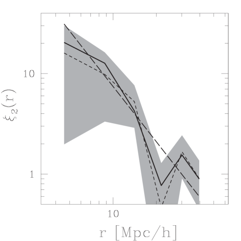
As an illustration of this procedure we calculate the two–point correlation function $\xi_{2}$ from the sample L20. The $\xi_{2}$ together with the number density satisfy the constraint (20) (see Table 2): $\varrho C_{2}<1$. We use this empirical $\xi_{2}$ as an input to the simulation algorithm outlined above. Fig. 7 illustrates that these simulated Gauss–Poisson sets are indeed able to reproduce the observed two–point correlation function. Even the dip of $\xi_{2}$ at 20$h^{-1}$Mpc, is well reproduced by the simulated point sets. By construction no higher–order correlations are present in the simulated point sets in the mean.

Figure 7: The two–point correlation function $\xi_{2}(r)$ estimated from the L20 sample (solid line) is shown together with $\xi_{2}(r)$ estimated from 200 realizations of a Gauss–Poisson process with the same $\xi_{2}$ and number density as for the observed clusters (short dashed line, shaded one–$\sigma$ area). The long dashed line is for $\xi_{2}(r)=(30/r)^{1.83}$.

3.4 Minkowski functionals of a Gauss–Poisson process

In the following the Minkowski functionals for a Gauss–Poisson process will be given. Truncating after the second term in Eq. (15) one obtains the correlated average of the specific Minkowski functionals

$${\overline{M}}_{\nu}(r;\varrho,\xi_{2})= 1-2^{\nu-1}\eta\ \delta{\overline{M}}_{\nu}^{(GP)}(r;\xi_{2}),$$ (23)

$$\delta{\overline{M}}_{\nu}^{(GP)}(r;\xi_{2})= \frac{1}{2^{\nu}M_{0}(B_{r})}\int\limits_{B_{2r}(\mathbf{0})}{\rm d}{\mathbf{x}}\ \xi_{2}(|{\mathbf{x}}|)\ I_{\nu}(r;|{\mathbf{x}}|)$$

with the volume $M_{0}(B_{r})$ of a sphere of radius $r$. From Eq. (23) and using the expressions for $I_{\nu}(r;s)$ given in Eq. (11) we can calculate the normalized Minkowski functionals of the Gauss–Poisson process according to Eq. (16). For example we obtain

$$\Phi_{0}(r;\varrho,\xi_{2})=\big{(}1-{\rm e}^{-\eta{\overline{M}}_{0}}\big{)}/\eta,$$

with

$${\overline{M}}_{0}=1-\frac{\eta\ 4\pi}{2M_{0}(B_{r})}\int_{0}^{2r}{\rm d}s\ s^{2}\xi_{2}(s)\Big{(}1-\frac{3}{2}\frac{s}{2r}+\frac{1}{2}\big{(}\frac{s}{2r}\big{)}^{3}\Big{)},$$

and similar expressions for $\Phi_{1}$, $\Phi_{2}$, and $\Phi_{3}$.

The expansion (10) to linear order in $\eta\propto r^{3}\varrho$ allows us to describe the MFs only for small radii or low number densities. For a Gauss–Poisson process both $I_{\mu}$ and $\eta$ appear non–linearly in Eq. (16) via Eqs. (5, 23, 23). Contrary to the approximation (10) which is only valid for $\eta\ll 1$, the Minkowski functionals of the Gauss–Poisson process, are valid for all $\eta$. A Gauss–Poisson process does not imply the linearity of the MFs in $I_{\mu}$ and $\eta$.

For a Poisson distribution with $\xi_{2}(r)=0$ one obtains

$${\overline{M}}_{\nu}^{(P)}(r)=1\;,\;\;\delta{\overline{M}}_{\nu}^{(P)}(r)=0\;,$$ (24)

i.e., one recovers Eq. (9). Assuming an algebraic scaling form

$$\xi_{2}(s)=\Big{(}\frac{s_{0}}{s}\Big{)}^{\gamma}$$ (25)

for the centered two–point correlation function one obtains with $\gamma<3$ the general result

$$\delta{\overline{M}}_{\nu}^{(GP)}(r)=A_{\nu}(\gamma)\ \Big{(}\frac{s_{0}}{2r}\Big{)}^{\gamma}$$ (26)

with the amplitudes

$$\begin{array}[]{ll}A_{0}(\gamma)=&\frac{24}{3-\gamma}-\frac{36}{4-\gamma}+\frac{12}{6-\gamma},\\ A_{1}(\gamma)=&\frac{12}{3-\gamma}-\frac{12}{4-\gamma},\\ A_{2}(\gamma)=&\frac{6}{3-\gamma}-\frac{6}{4-\gamma}+3\int\limits_{0}^{\pi/2}{\rm d}y\ y\cos^{2}y\sin^{2-\gamma}y,\\ A_{3}(\gamma)=&\frac{3}{3-\gamma}.\\ \end{array}$$ (27)

In the limiting case $\gamma\rightarrow 0$ (with $\varrho\rightarrow 0$) one recovers the result $A_{0}=A_{1}=A_{3}=1$ and $A_{2}=\frac{1}{2}+\frac{3\pi^{2}}{64}$ for the averaged Minkowski functionals

$$A_{\nu}\;=\;2^{-\nu}\int{\rm d}{\mathbf{x}}\;\frac{M_{\nu}(B_{r}(\mathbf{0})\cap B_{r}({\mathbf{x}}))}{M_{\nu}(B_{r})M_{0}(B_{r})}$$ (28)

of the intersection of two overlapping spheres with distance $|{\mathbf{x}}|$ and radius $r$ (see kinematic formula (6)).

One has to be careful in the interpretation of Eq. (27), since a scale–invariant two–point correlation function (25) with $\gamma<3$ does not satisfy the constraint (20), as required for the existence of a Gauss–Poisson process. A cut–off, i.e. $\xi_{2}(s)=0$ for $s>r_{c}$, has to be imposed below some radius $r_{c}$ to guarantee the constraint (20). The maximal allowed $r_{c}$ is depending on the number density through (20). As can be seen directly from Eq. (23), the scaling behavior (26) as well as the amplitudes $A_{\nu}$ in Eq. (27) are still correct for $2r<r_{c}$. Only on larger scales additional terms depending on the cut–off will emerge. In such a scale invariant Gauss–Poisson process the specific MFs $\delta{\overline{M}}_{\nu}(r)$ should show the general scaling form (26) which may be used to test for an algebraic two–point correlation function $\xi_{2}(r)$.

The actual measured specific MFs still depend on the density $\varrho$ and all of the correlation functions $\xi^{(n)}({\mathbf{x}}_{1},\ldots,{\mathbf{x}}_{n})$. The deviations of the measured MFs from the expressions (23) for a Gauss–Poisson process will be used as a measure for the relevance of higher–order correlations among the points (see Sect. 4).

To facilitate future applications we will also quote the Minkowski functionals of a Gauss–Poisson process in two dimensions (Mecke, 1994). With $\eta=\pi r^{2}\varrho$ the reduced Minkowski functionals (compare Eq. (16) for three dimensions)

$$\begin{array}[]{l}\Phi_{0}(r;\varrho,\{\xi_{n}\})=(1-{\rm e}^{-\eta{\overline{M}}_{0}})/\eta\\ \Phi_{1}(r;\varrho,\{\xi_{n}\})={\overline{M}}_{1}{\rm e}^{-\eta{\overline{M}}_{0}}\\ \Phi_{2}(r;\varrho,\{\xi_{n}\})=({\overline{M}}_{2}-\eta{\overline{M}}_{1}^{2}){\rm e}^{-\eta{\overline{M}}_{0}},\end{array}$$ (29)

with the specific Minkowski functionals given by Eq. (15). For a Gauss–Poisson process the specific Minkowski functionals are given by the Eq. (23), the volume $M_{0}(B_{r})=\pi r^{2}$ of a disc of radius $r$, and the functions

$$\begin{array}[]{rl}I_{0}(r;s)=&1-\frac{2}{\pi}\bigg{(}\arcsin\frac{s}{2r}-\frac{s}{2r}\Big{(}1-\big{(}\frac{s}{2r}\big{)}^{2}\Big{)}^{\tfrac{1}{2}}\bigg{)}\\ I_{1}(r;s)=&1-\frac{2}{\pi}\arcsin\frac{s}{2r}\\ I_{2}(r;s)=&\Theta(2r-s).\\ \end{array}$$ (30)

If the correlation function decays algebraicly $\xi(r)=(s_{0}/r)^{\gamma}$, $r=|{\mathbf{x}}_{1}-{\mathbf{x}}_{2}|$, with an scaling exponent $\gamma$ and a correlation length $s_{0}$ one finds for the intensities of the Minkowski measures (16) for homogeneously distributed discs $B_{r}$ of radius $r$ in two dimensions the amplitudes (Mecke, 1994)

$$\begin{array}[]{ll}A_{0}(\gamma)=&\frac{8}{2-\gamma}-2g(\gamma)-f(\gamma),\\ A_{1}(\gamma)=&\frac{4}{2-\gamma}-g(\gamma),\\ A_{2}(\gamma)=&\frac{2}{2-\gamma},\end{array}$$ (31)

with the functions

$$f(\gamma)=\frac{4}{\sqrt{\pi}}\frac{\Gamma\big{(}\tfrac{3}{2}-\tfrac{\gamma}{2}\big{)}}{\Gamma\big{(}3-\tfrac{\gamma}{2}\big{)}},$$ (32)

and

$$g(\gamma) =\frac{8}{\pi}\int\limits_{0}^{1}{\rm d}y\ y^{1-\gamma}\arcsin(y).$$ (33)

One also recovers the result $A_{\nu}=1$ in the limit $\gamma\rightarrow 0$ (with $\varrho\rightarrow 0$) for the averaged Minkowski functionals of the intersection of two discs defined in Eq. (28). In general a cut–off in the scale invariant correlation function is needed to make this model well–defined. See the comments above.

4 Non–Gaussian morphology of the galaxy cluster distribution

In this section we compare the Minkowski functionals determined from the cluster distribution with the Minkowski functionals of a Gauss–Poisson process. In Sect. 3.2 we showed that the number density $\varrho$ and the two–point correlation function $\xi_{2}(r)$ have to fulfill constraints in order to allow them to serve as the ingredients for a Gauss–Poisson point process. The constraint (41) implies $\xi_{2}(r)\geq 0$ for all $r$. There are indications from the analysis of the flux–limited Reflex catalogue that the two–point correlation function of the cluster distribution becomes negative on scales of 40–50$h^{-1}$Mpc (Collins et al., 2000). The violation of constraint (41) already tells us that the cluster distribution exhibits non–Gaussian features even on such large scales. Due to the limited number of clusters and the smaller extent of samples we can not detect this zero crossing unambiguously in the volume–limited samples we analyzed. To obtain a well–defined model of the two–point correlation function we impose a cut at $r_{c}=48{{h^{-1}{\rm Mpc}}}$ with $\xi_{2}(r)=0$ at $r>r_{c}$.

Another more stringent constraint is Eq. (40) which may be cast into the form

$$\varrho\ \int_{{\mathbb{R}}^{3}}{\rm d}{\mathbf{y}}\ \xi_{2}(|{\mathbf{y}}|)=\varrho\ C_{2}\leq 1.$$ (34)

As can be seen from Table 2, the smaller volume–limited samples L05–L12, with their higher number density clearly violate this constraint. Hence, already by inspecting the two–point correlation function $\xi_{2}$ in conjunction with the number density $\varrho$ we can conclude that there are non–negligible higher–order correlations in the point distribution of galaxy cluster in the samples L05 and L12.

In Sect 3.3 we showed how to simulate a Gauss–Poisson process for a given two–point correlation function $\xi_{2}$ and $\varrho$. The violation of the constraint (34) prohibits the simulation of a Gauss–Poisson process corresponding to the samples L05 and L12. However for the samples L20 and L30 the constraint (34) is satisfied (see Table 2) and we may generate realizations of a Gauss–Poisson process with the same number density and the same two–point correlation function, as estimated from these samples, (see Sect. 3.2 and especially Fig. 7). Both constraints (20) and (21) are only necessary conditions for the existence of a Gauss–Poisson process. Still higher–order correlations may be present in the cluster distribution. We calculate the Minkowski functionals of these Gauss–Poisson samples and compare them with the Minkowski functionals of the observed cluster distribution. Since correlations of any order enter the Minkowski functionals (see Eq. (5) or Eqs. (15) and (16)), deviations of the Minkowski functionals of the cluster distribution from the Minkowski functionals of the Gauss–Poisson process indicate the presence of higher–order correlations even in these deep samples. To facilitate the comparison we use the normalized Minkowski functionals

$$\Phi_{\nu}(r)=\frac{{m}_{\nu}({\cal A}_{r})}{M_{\nu}(B_{r})\;\varrho(r)}.$$ (35)

To get unbiased estimates of the MFs we employ a boundary corrected estimator where we shrink the observational window $W(r)$ with increasing radius $r$ of the spheres (Mecke et al. 1994, Schmalzing & Diaferio 2000). As an estimate of the number density inside $W(r)$ we use $\varrho(r)=N(r)/|W(r)|$ with $N(r)$ the number of points inside the shrunken window with the volume $|W(r)|$.

Figure 8: The reduced Minkowski functionals $\Phi_{\mu}$ of the volume–limited sample L20 (solid line, see also Fig. 5) compared to the Minkowski functionals of a Gauss–Poisson process (short dashed line, shaded one–$\sigma$ area) with the empirical two–point correlation function as input (see Fig. 7). The long dashed line is obtained from the scale invariant model (see Eq. (26)) with $s_{0}=30{{h^{-1}{\rm Mpc}}}$, $\gamma=1.83$ and the amplitudes $A_{0}=6.8$, $A_{1}=4.73$, $A_{2}=2.70$, and $A_{3}=2.56$ according to Eq. (27). The mean Minkowski functionals of a Poisson process are shown as a dotted line. The errors for the Poisson process (not shown) are smaller than the errors from the Gauss–Poisson process.

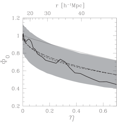
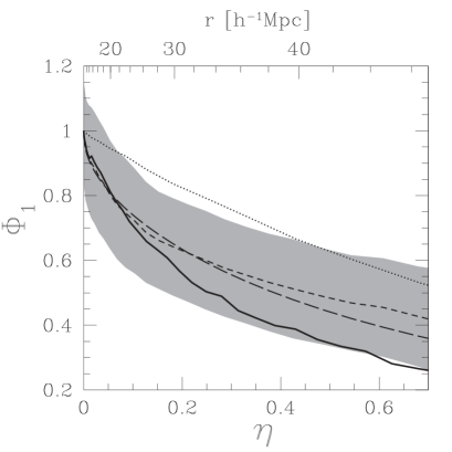
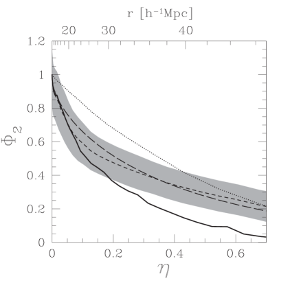
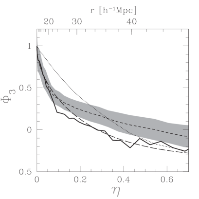
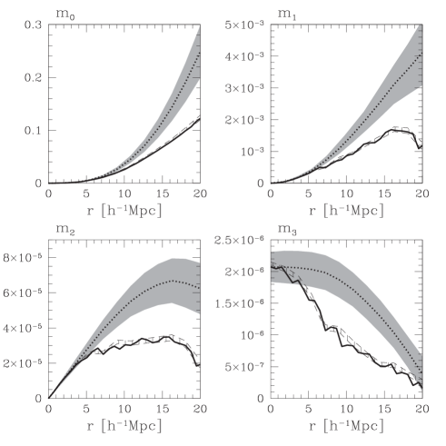
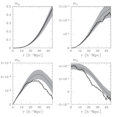
In Fig. 8 the results of our comparison are shown, where the $\Phi_{\mu}$’s are plotted against $\eta=\varrho(4\pi/3)r^{3}$. We used the empirical two–point correlation function to generate the realizations of the Gauss–Poisson process inside the sample geometry of the Reflex cluster catalog. The shaded one–$\sigma$ area with the short dashed line in the center was estimated from one hundred realizations. The initial slope of the MFs of the cluster distribution (solid line) is well approximated by the expression (10). But already for fairly small $\eta$ this linear approximation breaks down. As discussed in Sect. 3.4 a Gauss–Poisson process does not imply the linearity of the MFs in $\eta$, which is readily observed in Fig. 8. It is necessary to compare the measured values of $M_{\nu}(r)$ with Eq. (16) which is available in the analytic form only because of additivity. So our heuristic argument in the beginning (to look for additive integral information on higher correlations) turns out to be useful in deriving analytic results which are necessary for the comparison with measured values. Over the whole range of scales probed, the normalized volume $\Phi_{0}$ and surface area $\Phi_{1}$ of the cluster samples are consistent with the Gauss–Poisson process. However, both the normalized integral mean curvature $\Phi_{2}$ and the normalized Euler characteristic $\Phi_{3}$ are lowered with respect to the Gauss–Poisson process, clearly outside the one–$\sigma$ range. The deviations are especially prominent for radii larger than 30$h^{-1}$Mpc. This is a firm indication that higher–order correlations are necessary to account for the shape and topology of the cluster distribution for such large scales, given by the radii of the spheres.

In Fig. 8 also the MFs of a Gauss–Poisson process with a scale invariant two–point correlation function $\xi_{2}(r)=(s_{0}/r)^{\gamma}$ are shown (see Eqs. (26), (27) and (16)). The exponent is $\gamma=1.83$ as determined by Collins et al. (2000) and $s_{0}=30{{h^{-1}{\rm Mpc}}}$. These parameters give a reasonable fit to the wiggly two–point correlation function determined from volume–limited sample L20 (Fig. 7). The normalized volume $\Phi_{0}$, surface area $\Phi_{1}$ and integral mean curvature $\Phi_{2}$ of a Gauss–Poisson process with this scale invariant $\xi_{2}$ follow closely the corresponding quantities determined from the Gauss–Poisson process using the two–point correlation function from the data. A significant difference between the two Gaussian models shows up only in the Euler characteristic $\Phi_{3}$.

To quantify the deviation of the distribution of galaxy clusters from a Gauss–Poisson process we perform a non–parametric significance test (Besag & Diggle, 1977; Stoyan, 2000). Using $M=10$ equidistant radii $r_{i}$ in the range from 30$h^{-1}$Mpc to 45$h^{-1}$Mpc we define the “distance”

$$d_{\nu}^{k}=\frac{1}{M}\sum_{i=1}^{M}\Big{(}\Phi_{\nu}^{k}(r_{i})-\Phi_{\nu}^{\text{GP}}(r_{i})\Big{)}^{2}$$ (36)

between the normalized Minkowski functionals $\Phi_{\nu}^{k}$ of the sample labeled with $k$ and the mean value $\Phi_{\nu}^{\text{GP}}$ of the Gauss–Poisson process calculated from one hundred realizations inside the same sample geometry as the Reflex samples and using the empirical $\varrho$ and $\xi_{2}$. Additional to the distances $d_{\nu}^{\text{L20}}$ of the cluster sample L20, we also calculate the distances $d_{\nu}^{k}$ for $k=1\ldots 99$ realizations of the Gauss–Poisson process (these 99 realizations are independent from the realizations used to calculate the mean $\Phi_{\nu}^{\text{GP}}$). We order these distances including $d_{\nu}^{\text{L20}}$ ascending. If $d_{\nu}^{\text{L20}}$ is under the five highest distance values, we may exclude a Gauss–Poisson process with a significance of 95% (see the comments by Marriott 1978 concerning the significance level). The beauty of this Monte–Carlo significance test is that we neither make assumptions about the distribution of the Reflex clusters, nor about the distribution of the errors of the MFs in the model.

Table 3: The rank of the cluster sample L20 within the ascending list of one hundred ordered distances $d_{\nu}^{k}$. A rank larger than 95 indicates rejection with significance of 95%.

$\nu$	0	1	2	3
rank	26	52	97	96

In Table 3 the rank of the cluster sample L20 within the ordered list of distances is given. As expected from the visual impression in Fig. 8 the volume $\Phi_{0}$ and the surface area $\Phi_{1}$ are consistent with the expectation from a Gauss–Poisson process. Both the integral mean curvature $\Phi_{2}$ and the Euler characteristic $\Phi_{3}$ allows us to reject the hypotheses that the cluster distribution stems from a Gauss–Poisson process at a significance level of 95%. This result is stable against extending or shrinking the radial range. One may also use the overall mean number density $\varrho$ of the full sample in Eq. (35) instead of $\varrho(r)$.

We implemented this Monte–Carlo test using the empirical two–point correlation function as input to the simulations of the Gauss–Poisson process. For a scale–invariant $\xi_{2}(r)=(30{{h^{-1}{\rm Mpc}}}/r)^{1.83}$ the normalized Euler characteristic $\Phi_{3}$ according to Eq. (26) seems to be in agreement with the observed MFs. However, the family of MFs provides us with a consistency check, still the integral mean curvature $\Phi_{2}$ from the scale invariant model and the data are differing, illustrating the relevance of higher–order correlations. Hence, also a Gauss–Poisson process with a scale–invariant correlation function is inconsistent with the data.

Figure 9: The reduced Minkowski functionals $\Phi_{\mu}$ of the volume–limited sample L30 (see also Fig. 6). The same conventions as in Fig. 8 apply.

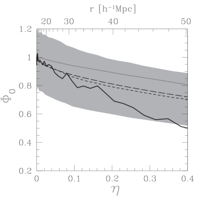
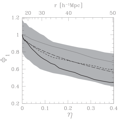
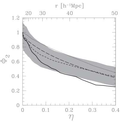
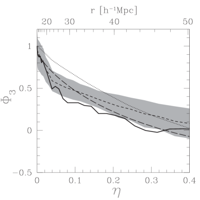
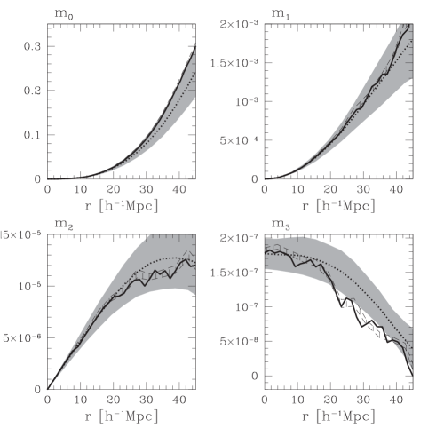
We conducted a similar analysis for the cluster sample L30 (see Fig. 9). Again $\Phi_{0}$ and $\Phi_{1}$ fall within the one–$\sigma$ range of the Gauss–Poisson process. The $\Phi_{2}$ and $\Phi_{3}$ only marginally stand out. As discussed in Sect. 2.3 this sample hardly allows for a discrimination from the Poisson process, which can be explained by Eq. (10) and the significantly lowered number density. Nevertheless the same tendency can be observed as for the sample L20 although the statistics does not allow a discrimination.

5 Summary

The Reflex cluster catalogue is well suited for studying the large–scale structure of the Universe. The detection of the clusters is based on their X–ray flux, allowing the construction of a flux–limited sample. X–ray selected cluster catalogues are not impaired by projection effects. Moreover, the flux–limit, together with the well documented selection effects allows the extraction of clean volume–limited samples.

We calculated Minkowski functionals of a series of volume–limited samples, extracted from the Reflex cluster catalogue. The comparison with the MFs of Poisson distributed points revealed similar features as detected in the Abell/ACO cluster sample (Kerscher et al., 1997). Although the number of clusters in the samples is always less than one hundred, MFs allow for a sensitive and discriminatory analysis. The stability of the results obtained from this small number of points can be attributed to the additivity property of the MFs, which served as a construction principle.

Our aim was the quantification of non–Gaussian features in the large–scale distribution of clusters, therefore we first gave a precise definition of a Gaussian point distribution, the Gauss–Poisson process. Contrary to a Gaussian random field, constraints for number density and the two–point correlation function arise. In the smaller volume–limited samples L05 and L12 these constraints are violated. Hence, a Gauss–Poisson process with the observed density and two–point correlation function does not exist. This is an indirect detection of higher–order correlation functions. Higher–order correlation functions are needed to allow for the increased variance. Clearly, the relevance of these higher–order correlations has to be checked independently, e.g. using the MFs. Due to the decreasing number density of galaxy clusters the deeper volume–limited samples L20 and L30 comply with the constraints. A Gauss–Poisson process based on the observed correlation function becomes feasible as a model. MFs summarize the influence of the two–point correlations and higher–order correlations on the morphology of large–scale structure. They include correlations of any order in an integral way. We calculated the MFs for a general correlated point set. Detailed results were given for the Gauss–Poisson process. To quantify higher–order correlations in the cluster distribution we compare the analytical known MFs known for the Gauss–Poisson process with the actual observed MFs of the cluster distribution. Two of the four MFs, the volume and the surface area, are consistent with the Gaussian model. However a clear detection of non–Gaussian features at large scales was possible with the integral mean curvature and the Euler characteristic.

The definition of the Gauss–Poisson process directly lead to a method for simulating Gaussian point distributions. With such simulated point distributions we performed a non–parametric Monte–Carlo test. The main result is that we can exclude a Gauss–Poisson process as a viable model for the distribution of galaxy clusters at the significance level of 95%.

Non–Gaussian features seen in the distribution of galaxy clusters may be already imprinted on the initial density field (see e.g. Linde & Mukhanov 1997), or may be a result of topological defects (see e.g. Shellard & Brandenberger 1988). We would like to point out that also explanations facilitating Gaussian initial conditions are possible. Introducing a threshold and considering only peaks in a Gaussian density field Bardeen et al. (1986) could show that the point distribution of the peaks has non zero higher–order correlations $\xi_{n}\neq 0$ for $n>2$. Still the importance of the higher–order correlations on large scales comes as a surprise within this model. On physical grounds, the peak biasing picture may only serve as a first approximation. Evolving a Gaussian density field in time using the linear approximation leads to larger and larger regions with a non–physical negative mass density. Only the non–linear evolution of the density field can remedy these shortcomings, allowing on the one hand for high density peaks with an over–density of several hundreds, and on the other hand allowing voids with a negative density contrast always larger than minus one. At the peaks of this non–linear evolved density fields one may assume the clusters to reside. As already discussed in the introduction non–Gaussian features in the large–scale distribution of mass, like walls and filaments, are predicted both by the Zel’dovich and related approximations as well as by $N$–body simulations, both based on Gaussian initial conditions. These structures in the mass distribution, perhaps amplified by a biasing mechanism, can be associated with the non–Gaussian structures observed in the large–scale distribution of Reflex galaxy clusters. Our results suggest that within these scenarios, using Gaussian initial conditions, it is necessary to consider non–linear models to describe the observed large–scale structures.

Acknowledgments

We thank Jörg Retzlaff for help in generating Fig. 1. MK acknowledges support from the NSF grant AST 9802980 and from the Sonderforschungsbereich 375 für Astroteilchenphysik der DFG. KM acknowledges support from the DFG grant ME1361/6-1.

Appendix A The constraints

In this appendix we recall the derivation of the constraints on the number density $\varrho$ and $\xi_{2}(r)$ for the Gauss–Poisson process as presented by Milne & Westcott (1972) (see also Kerscher 2001).

Consider $k$ compact disjoint sets $A_{j}$, and let $n_{j}=N(A_{j})$ be the number of points inside $A_{j}$. The probability generating function of the $k$-dimensional random vector $(n_{1},\cdots,n_{k})$ is then

$$P_{k}({\mathbf{z}})=P_{k}(z_{1},\ldots,z_{k})={\mathbb{E}}\bigg{[}\prod_{j=1}^{k}z_{j}^{n_{j}}\bigg{]}.$$ (37)

Together with a continuity requirement the knowledge of all finite–dimensional probability generating functions $P_{k}$ determines the p.g.fl. $G[h]$ (see Eq. (18)) and the point process completely (e.g. Westcott 1970). Setting

$$h({\mathbf{x}})=1-\sum_{j=1}^{k}(1-z_{j})\mbox{1l}_{A_{j}}({\mathbf{x}}),$$ (38)

one obtains the probability generating function of these finite–dimensional distributions from the probability generating functional of the point process: $P_{k}({\mathbf{z}})=G[h]$. Here $\mbox{1l}_{A}({\mathbf{x}})$ is the indicator–function of the set $A$, with $\mbox{1l}_{A}({\mathbf{x}})=1$ for ${\mathbf{x}}\in{A}$ and zero otherwise.

Since $P_{k}({\mathbf{z}})$ is a probability generating function of a random vector, it is positive and monotonically increasing in each component $z_{i}$, hence $\log P_{k}({\mathbf{z}})$ is non–decreasing. Inserting Eq. (38) into the probability generating functional of the Gauss–Poisson process (19) one immediately obtains

$$\frac{\partial\log P_{k}({\mathbf{z}})}{\partial z_{l}}=\varrho|A_{l}|+\\ +\varrho^{2}\sum_{j=1}^{k}\int_{A_{l}}{\rm d}{\mathbf{x}}\int_{A_{j}}{\rm d}{\mathbf{y}}\ \xi_{2}(|{\mathbf{x}}-{\mathbf{y}}|)(z_{j}-1)\geq 0$$ (39)

for any $z_{j}\geq 0$, where $|A_{l}|$ is the volume of the set $A_{l}$. We chose $z_{j}=1$ for all $j\neq i$ and set the remaining $z_{i}$ either to $z_{i}=0$ or $z_{i}\gg 1$. Then the following two constraints emerge:

$$\frac{\varrho}{|A_{i}|}\ \int_{A_{i}}{\rm d}{\mathbf{x}}\int_{A_{j}}{\rm d}{\mathbf{y}}\ \xi_{2}(|{\mathbf{x}}-{\mathbf{y}}|) \leq 1,$$ (40)

$$\int_{A_{i}}{\rm d}{\mathbf{x}}\int_{A_{j}}{\rm d}{\mathbf{y}}\ \xi_{2}(|{\mathbf{x}}-{\mathbf{y}}|) \geq 0,$$ (41)

for any subset $A_{i},A_{j}$ of ${\mathbb{R}}^{3}$. Milne & Westcott (1972) showed that these two conditions are necessary and sufficient for the existence of the Gauss–Poisson process.

With $A_{i}$ as an infinitesimal volume element centered on the origin and $A_{j}$ equal to some volume $A$ the first constraint (40) implies the simplified constraint (20). Considering two volume elements $A_{i}={\rm d}V_{i}$ and $A_{j}={\rm d}V_{j}$, then Eq. (41) implies Eq. (21).

References

- Abell (1958) Abell, G. O. 1958, ApJS, 3, 211
- Abell et al. (1989) Abell, G. O., Corwin Jr., H. G., & Olowin, R. P. 1989, ApJS, 70, 1
- Arnol’d et al. (1982) Arnol’d, V. I., Shandarin, S. F., & Zel’dovich, Ya. B. 1982, Geophysical and Astrophysical Fluid Dynamics, 20, 111
- Arns et al. (2001a) Arns, C., Knackstedt, M., Pinczewski, W., & Mecke, K. 2001a, Phys. Rev. E, 63, 31112
- Arns et al. (2001b) —. 2001b, submitted to PRL
- Baddeley & Silverman (1984) Baddeley, A. J. & Silverman, B. W. 1984, Biometrics, 40, 1089
- Bahcall (2000) Bahcall, N. A. 2000, Physics Rep., 333, 233
- Balian & Schaeffer (1989) Balian, R. & Schaeffer, R. 1989, A&A, 220, 1
- Bardeen et al. (1986) Bardeen, J. M., Bond, J. R., Kaiser, N., & Szalay, A. S. 1986, ApJ, 304, 15
- Beisbart et al. (2001) Beisbart, C., Buchert, T., Wagner, H., 2001, Physica A 293, 592
- Besag & Diggle (1977) Besag, J. & Diggle, P. J. 1977, Appl. Statist., 26, 327
- Blaschke (1936) Blaschke, W. 1936, Integralgeometrie. Erstes Heft (Leipzig, Berlin: Bernd G. Teubner)
- Böhringer et al. (2001) Böhringer, H., Schuecker, P., Guzzo, L., et al. 2001, A&A, 826
- Böhringer et al. (2000) Böhringer, H., Voges, W., Huchra, J.P., et al. 2000, ApJS, 435
- Bond et al. (1996) Bond, J. R., Kofman, L., & Pogosyan, D. Yu. 1996, Nature, 380, 603
- Borgani et al. (1999) Borgani, S., Rosati, P., Tozzi, P., & Norman, C. 1999, ApJ, 517, 40
- Broadhurst et al. (1990) Broadhurst, T. J., Ellis, R. S., Koo, D. C., & Szalay, A. S. 1990, Nature, 343, 726
- Collins et al. (2000) Collins, C., Guzzo, L., Böhringer, H., et al. 2000, MNRAS, 319, 939
- Daley & Vere-Jones (1988) Daley, D. J. & Vere-Jones, D. 1988, An Introduction to the Theory of Point Processes (Berlin: Springer Verlag)
- Dalton et al. (1997) Dalton, G., Maddox, S., Sutherland, W., & Efstathiou, G. 1997, MNRAS, 289, 263
- Doroshkevich et al. (1996) Doroshkevich, A. G., Fong, R., Gottlöber, S., Mücket, J. P., & Müller, V. 1996, MNRAS, 284, 633
- Eddington (1940) Eddington, A. S. 1940, MNRAS, 100, 354
- Einasto et al. (1997) Einasto, J., Einasto, M., Gottlöber, S., et al. 1997, Nature, 385, 139
- Gal et al. (2000) Gal, R. R., de Carvalho, R., Odewahn, S., Djorgovski, S., & Margoniner, V. 2000, AJ, 119, 12
- Hadwiger (1957) Hadwiger, H. 1957, Vorlesungen über Inhalt, Oberfläche und Isoperimetrie (Berlin: Springer Verlag)
- Hamilton et al. (1986) Hamilton, A. J. S., Gott III, J., & Weinberg, D. 1986, ApJ, 309, 1
- Huchra et al. (1990) Huchra, J. P., Geller, M. J., De Lapparent, V., & Corwin Jr., H. G. 1990, ApJS, 72, 433
- Jenkins et al. (1998) Jenkins, A., Frenk, C. S., Pearce, F. R., et al. 1998, ApJ, 499, 20
- Kaiser (1984) Kaiser, N. 1984, ApJ, 284, L9
- Katgert et al. (1996) Katgert, P., Mazure, A., Perea, J., et al. 1996, A&A, 310, 8
- Kendall & Stuart (1977) Kendall, M. G. & Stuart, A. 1977, The Advanced Theory of Statistics, 4th edn., Vol. 1 (New York: MacMillan)
- Kerscher (2000) Kerscher, M. 2000, in Statistical Physics and Spatial Statistics: The art of analyzing and modeling spatial structures and pattern formation, ed. K. R. Mecke & D. Stoyan, Lecture Notes in Physics No. 554 (Berlin: Springer Verlag), astro-ph/9912329
- Kerscher (2001) Kerscher, M. 2001, astro-ph/0102153, submitted to PRE
- Kerscher et al. (2001a) Kerscher, M., Buchert, T., & Futamase, T. 2001a, astro-ph/0007284, submitted to ApJL
- Kerscher et al. (2001b) Kerscher, M., Mecke, K., Schmalzing, J., et al. 2001b, A&A, 373, 1
- Kerscher et al. (1998) Kerscher, M., Schmalzing, J., Buchert, T., & Wagner, H. 1998, A&A, 333, 1
- Kerscher et al. (1997) Kerscher, M., Schmalzing, J., Retzlaff, J., et al. 1997, MNRAS, 284, 73
- Kitayama & Suto (1997) Kitayama, T. & Suto, Y. 1997, ApJ, 490, 557
- Kofman et al. (1992) Kofman, L., Pogosyan, D., Shandarin, S. F., & Melott, A. L. 1992, ApJ, 393, 437
- Kolb & Turner (1990) Kolb, E. W. & Turner, M. S. 1990, The Early Universe (Reading, MA: Addison–Wesley)
- Linde & Mukhanov (1997) Linde, A. & Mukhanov, V. F. 1997, Phys. Rev. D, 56, 535
- Marriott (1978) Marriott, F. H. C. 1978, Appl. Statist., 28, 75
- Mecke (2000) Mecke, K. 2000, in Statistical Physics and Spatial Statistics: The art of analyzing and modeling spatial structures and pattern formation, ed. K. Mecke & D. Stoyan, Lecture Notes in Physics No. 554 (Berlin: Springer Verlag)
- Mecke (1994) Mecke, K. R. 1994, Integralgeometrie in der Statistischen Physik: Perkolation, komplexe Flüssigkeiten und die Struktur des Universums (Thun, Frankfurt/Main: Harri Deutsch)
- Mecke et al. (1994) Mecke, K. R., Buchert, T., & Wagner, H. 1994, A&A, 288, 697
- Mecke & Wagner (1991) Mecke, K. R. & Wagner, H. 1991, J. Stat. Phys., 64, 843
- Melott (1990) Melott, A. L. 1990, Physics Rep., 193, 1
- Melott & Shandarin (1990) Melott, A. L. & Shandarin, S. F. 1990, Nature, 346, 633
- Milne & Westcott (1972) Milne, R. K. & Westcott, M. 1972, Adv. Appl. Prob., 4, 151
- Newman (1970) Newman, D. S. 1970, J. Appl. Prob., 7, 338
- Pan & Coles (2000) Pan, J. & Coles, P. 2000, MNRAS, 318, L51
- Peebles (1980) Peebles, P. J. E. 1980, The Large Scale Structure of the Universe (Princeton, New Jersey: Princeton University Press)
- Plionis & Valdarnini (1991) Plionis, M. & Valdarnini, R. 1991, MNRAS, 249, 46
- Postman et al. (1992) Postman, M., Huchra, J. P., & Geller, M. J. 1992, ApJ, 384, 404
- Santaló (1976) Santaló, L. A. 1976, Integral Geometry and Geometric Probability (Reading, MA: Addison–Wesley)
- Schmalzing & Diaferio (2000) Schmalzing, J. & Diaferio, A. 2000, MNRAS, 312, 638
- Schmalzing et al. (1999) Schmalzing, J., Gottlöber, S., Kravtsov, A., & Klypin, A. 1999, MNRAS, 309, 1007
- Schuecker et al. (2001) Schuecker, P., Böhringer, H., Guzzo, L., et al. 2001, A&A, 368, 86
- Scoccimarro (2000) Scoccimarro, R. 2000, ApJ, 544, 597
- Serra (1982) Serra, J. 1982, Image analysis and mathematical morphology (New York and London: Academic Press)
- Serra (1988) —. 1988, Image analysis and mathematical morphology II (New York and London: Academic Press)
- Shandarin (1983) Shandarin, S. F. 1983, Sov. Astron. Lett., 9, 104
- Shectman et al. (1996) Shectman, S. A., Landy, S. D., Oemler, A., et al. 1996, ApJ, 470, 172
- Shellard & Brandenberger (1988) Shellard, E. & Brandenberger, R. 1988, Phys. Rev. D, 38, 3610
- Stoyan (2000) Stoyan, D. 2000, in Statistical Physics and Spatial Statistics: The art of analyzing and modeling spatial structures and pattern formation, ed. K. Mecke & D. Stoyan, Lecture Notes in Physics No. 554 (Berlin: Springer Verlag)
- Stoyan et al. (1995) Stoyan, D., Kendall, W. S., & Mecke, J. 1995, Stochastic Geometry and its Applications, 2nd edn. (Chichester: John Wiley & Sons)
- Szalay (1997) Szalay, A. S. 1997, in Proc. of the 18th Texas Symposium on Relativistic Astrophysics, ed. A. Olinto (New York: AIP)
- Szapudi & Szalay (1993) Szapudi, I. & Szalay, A. S. 1993, ApJ, 408, 43
- Toth et al. (1989) Toth, G., Hollosi, J., & Szalay, A. S. 1989, ApJ, 344, 75
- van Haarlem et al. (1997) van Haarlem, M., Frenk, C., & White, S. 1997, MNRAS, 287, 817
- Voges et al. (1999) Voges, W., Aschenbach, B., Boller, T., et al. 1999, A&A, 249, 389
- Westcott (1970) Westcott, M. 1970, J. Aust. Math. Soc., 14, 448
- Zel’dovich (1970) Zel’dovich, Ya. B. 1970, Astrophysics, 6, 164
- Zucca et al. (1997) Zucca, E., Zamorani, G., Vettolani, G., et al. 1997, A&A, 326, 477