Constraints on Cosmological and Biasing models using AGN clustering

Abstract

We attempt to put constraints on different cosmological and biasing models by combining the recent clustering results of X-ray sources in the local ($z\leq 0.1$) and distant universe ($z\sim 1$). To this end we compare the measured angular correlation function for bright (Akylas et al. 2000) and faint (Vikhlinin & Forman 1995) ROSAT X-ray sources respectively with those expected in three spatially flat cosmological models. Taking into account the different functional forms of the bias evolution, we find that there are two cosmological models which performs well the data. In particular, low-$\Omega_{\circ}$ cosmological models ($\Omega_{\Lambda}=1-\Omega_{\circ}=0.7$) which contain either (i) high $\sigma_{8}^{\rm mass}=1.13$ value with galaxy merging bias, $b(z)\propto(1+z)^{1.8}$ or (ii) low $\sigma_{8}^{\rm mass}=0.9$ with non-bias, $b(z)\equiv 1$ best reproduce the AGN clustering results. While $\tau$CDM models with different bias behaviour are ruled out at a high significance level.

Keywords: galaxies: clustering- X-ray sources - cosmology:theory - large-scale structure of universe

1 Introduction

The study of the distribution of matter on large scales, based on different extragalactic objects, provides important constraints on models of cosmic structure formation. In particular Active Galactic Nuclei (AGN) can be detected up to very high redshifts and therefore provide information on how the X-ray selected sources trace the underlying mass distribution as well as the evolution of large scale structure (cf. Hartwick & Schade 1989).

However, a serious problem here is how the luminous matter traces the underlying mass distribution. Many authors have claimed that the large scale clustering pattern of different mass tracers (galaxies or clusters) is characterized by a bias picture (cf. Kaiser 1984). In this framework, biasing is assumed to be statistical in nature; galaxies and clusters are identified as high peaks of an underlying, initially Gaussian, random density field. Biasing of galaxies with respect to the dark matter distribution was also found to be an essential ingredient of CDM models of galaxy formation in order to reproduce the observed galaxy distribution (cf. Benson et al. 2000). Furthermore, different studies have shown that the bias factor, $b(z)$, is a monotonically increasing function of redshift (cf. Fry 1996; Mo & White 1996; Matarrese et al. 1997; Moscardini et al. 1998; Tegmark & Peebles 1998; Basilakos & Plionis 2001). For example, Steidel et al. (1998) confirmed that the Lyman-break galaxies are very strongly biased tracers of mass and they found that $b(z=3.4)\raise-3.0pt\hbox{\hbox to0.0pt{\hbox{$\sim$}\hss}\raise 4.0pt\hbox{$>$}\ }6,4,2$, for SCDM, $\Lambda$CDM $(\Omega_{\circ}=0.3)$ and OCDM $(\Omega_{\circ}=0.2)$, respectively.

Studies based on the traditional indicators of clustering, like the two point correlation function, have been utilized in order to describe the AGN clustering properties. Our knowledge regarding the AGN clustering comes mostly from optical surveys for QSO’s (cf. Shanks & Boyle 1994; Croom & Shanks 1996; La Franca et al. 1998 and reference therein). It has been established, from Croom & Shanks (1996), that QSO’s have a clustering length of $r_{\circ}=5.4\pm 1.1h^{-1}$Mpc (with mean redshift of 1.27), while La Franca et al. (1998), analysing a sample of $\sim 700$ quasars in the redshift range $0.3\leq z\leq 3.2$, found $r_{\circ}=6.2\pm 1.6h^{-1}$Mpc. It is very important to note that comparison of these clustering results in different redshifts rather favours a comoving model for the evolution of clustering.

Similarly, Vikhlinin & Forman (1995) studied the angular clustering properties using a set of deep ROSAT observations. Carrera et al. (1998) combined two soft X-ray surveys (235 AGN), the ROSAT Deep Survey (Georgantopoulos et al. 1996) and the RIXOS survey (Mason et al. 2000) and found a spatial correlation length $1.5h^{-1}$Mpc $\leq r_{\circ}\leq 5.5h^{-1}$Mpc, depending on the adopted model of clustering evolution. Boyle & Mo (1993) analysing the EMSS survey which contains 183 low redshift AGNs, found a feeble clustering signal on scales $<10h^{-1}$Mpc. Recently, Akylas et al (2000) using 2096 sources detected in the ROSAT All Sky Survey Bright Source Catalogue (RASSBSC), derived the AGN angular correlation function in the nearby Universe and utilizing Limber’s equation obtained $r_{\circ}=6.7\pm 1.0h^{-1}$Mpc, assuming comoving clustering evolution.

In this paper we present the standard theoretical approach to estimate the angular correlation function $w(\theta)$, using different models for the bias evolution in different spatially flat cosmological models. Comparing the latter with observational results, we attempt to put constraints on the different cosmological and bias models. The plan of this paper is the following: In section 2, (a) we present the calculation of the theoretical predictions for $w(\theta)$, (b) we describe the models for bias evolution and (c) we discuss the AGN selection function. In section 3 we present the CDM spatially flat cosmologies, while in section 4 we present the predictions for $w(\theta)$. The observational results are compared with the predictions in section 5 and finally in section 6 we draw our conclusions.

2 The Integral Equation

For the purpose of this study we will utilize the relation between the angular $w(\theta)$ and spatial $\xi(r,z)$ two point correlation functions (cf. Maglioccheti et al. 1999 and references theirin). As it is well known, this connection can be done using the Limber equation (cf. Peebles 1980). For example, in the case of a spatially flat Universe ($\Omega_{\circ}+\Omega_{\Lambda}=1$), the Limber equation can be written as

$$w(\theta)=2\frac{\int_{0}^{\infty}\int_{0}^{\infty}x^{4}\phi^{2}(x)\xi(r,z){\rm d}x{\rm d}u}{[\int_{0}^{\infty}x^{2}\phi(x){\rm d}x]^{2}}\;\;,$$ (1)

where $\phi(x)$ is the selection function (the probability that a source at a distance $x$ is detected in the survey) and $x$ is the comoving coordinate related to the redshift through

$$x=\frac{c}{H_{\circ}}\int_{0}^{z}\frac{{\rm d}y}{E(y)}\;\;,$$ (2)

with

$$E(z)=[\Omega_{\circ}(1+z)^{3}+\Omega_{\Lambda}]^{1/2}$$ (3)

(see Peebles 1993). The mean surface density, ${\cal N}$, on a survey of solid angle $\Omega_{s}$ is:

$${\cal N}=\int_{0}^{\infty}x^{2}\phi(x){\rm d}x=\frac{1}{\Omega_{s}}\int_{0}^{\infty}N(z){\rm d}z\;\;,$$ (4)

where $N(z)$ is the number of objects in the given survey within the shell $(z,z+{\rm d}z)$. Therefore, combining the above system of equations, the expression for $w(\theta)$ satisfies the form

$$w(\theta)=2\frac{H_{\circ}}{c}\frac{\int_{0}^{\infty}N^{2}(z)E(z){\rm d}z\int_{0}^{\infty}\xi(r,z){\rm d}u}{[\int_{0}^{\infty}N(z){\rm d}z]^{2}}\;\;.$$ (5)

The physical separation between two sources, separated by an angle $\theta$ considering a small angle approximation is given by:

$$r\simeq\frac{1}{(1+z)}\left(u^{2}+x^{2}\theta^{2}\right)^{2}\;\;.$$ (6)

Extending this picture, we quantify the evolution of clustering with epoch presenting the spatial correlation function of the X-ray sources as

$$\xi(r,z)=\xi_{\rm mass}(r)R(z)\;\;,$$ (7)

with

$$R(z)=D^{2}(z)b^{2}(z)$$ (8)

where $D(z)$ is the linear growth rate of clustering (cf. Peebles 1993) being given by

$$D(z)=\frac{5\Omega_{\circ}E(z)}{2}\int^{\infty}_{z}\frac{(1+y)}{E^{3}(y)}{\rm d}y$$ (9)

and $b(z)$ is the evolution of bias. On large scales, we utilize the standard procedure based on the linear theory predictions from the power spectrum $P(k)$. On small scales we will follow the notation of Maglioccheti et al. (1999), who used the APM correlation function (Maddox et al. 1990) in order to estimate the angular correlation function of radio sources. In partcular, for $\Gamma=0.2$ the above extrapolation is used for $r\leq r_{\circ}^{\rm opt}=5.4h^{-1}$Mpc while for other values of $\Gamma$ we have re-scaled $\xi(r)$ using $\xi(r)\propto\xi(r\Gamma_{1}/\Gamma_{2})$.

2.1 Bias Evolution

The concept of biasing between different classes of extragalactic objects and the background matter distribution was put forward by Kaiser (1984) and Bardeen et al. (1986) in order to explain the higher amplitude of the 2-point correlation function of clusters of galaxies with respect to that of galaxies themselves.

The deterministic and linear nature of biasing has been challenged (cf. Bagla 1998; Dekel & Lahav 1999) and indeed on small scales ($r<10h^{-1}$Mpc) there are significant deviations from $b(r)=const$. Despite the above, the linear biasing assumption is still a useful first order approximation which, due to its simplicity, it is used in most studies of large scale clustering (cf. Magliocchetti et al. 1999). In this paper however, we will not indulge any variation of bias with scale but rather, working within the paradigm of linear and scale-independent bias. Therefore, we shortly describe some of the bias evolution models in order to introduce them to our analysis (see eq. 7 and eq. 8).

• No evolution of bias (B0): This model considers constant bias at all epochs:

  $$b(z)=b_{\circ}\simeq b_{\circ}^{\rm opt}\left(\frac{r_{\circ}}{r_{\circ}^{\rm opt}}\right)^{\gamma/2}$$ (10)

  where $r_{\circ}^{\rm opt}=5.4h^{-1}$Mpc is the correlation length in comoving coordinates estimated by the APM correlation function (Maddox et al. 1990) and $r_{\circ}$ is the corresponding length for the X-ray sources. Finally, $b_{\circ}^{\rm opt}=1/\sigma_{8}^{\rm mass}$ is the present bias of optical galaxies relative to the distribution of mass and $\sigma_{8}^{\rm mass}$ is the mass rms fluctuations in sphere of radius 8$h^{-1}$Mpc. Using the above ideas, if ones assumes that $r_{\circ}>r_{\circ}^{\rm opt}$, then it is quite obvious that the X-ray sources are indeed more biased with respect to optical galaxies by the factor $(r_{\circ}/r_{\circ}^{\rm opt})^{\gamma/2}$. In case that $b(z)\equiv 1$, we have the so called non-bias model.

• Test Particle or Galaxy Conserving Bias (B1): This model, proposed by Nusser & Davis (1994), Fry (1996), Tegmark & Peebles (1998), predicts the evolution of bias, independent of the mass and the origin of halos, assuming only that the test particles fluctuation field is related proportionally to that of the underlying mass. Thus, the bias factor as a function of redshift can be written:

  $$b(z)=1+\frac{(b_{\circ}-1)}{D(z)}\;\;\;\;,$$ (11)

  where $b_{\circ}$ is the bias factor at the present time. Bagla (1998) has found, that in the range $0\leq z\leq 1$, the above formula describes well the evolution of bias.

• Merging Bias Model (B2): Mo & White (1996) have developed a model for the evolution of the correlation bias, using the Press-Schechter formalism. Utilizing a similar formalism, Matarrese et al. (1997) extended the Mo & White results to include the effects of different mass scales (see also Moscardini et al. 1997; Bagla 1998; Catelan et al. 1998; Magliocchetti et al. 2000). In this case we have that

  $$b(z)=0.41+\frac{(b_{\circ}-0.41)}{D(z)^{\beta}}\;\;,$$ (12)

  with $\beta\simeq 1.8$.

2.2 Selection Function

In flux-limited samples, it is well known that there is a degradation of sampling as a function of distance from the observer (codified by the so called selection function). The latter also depends on the evolution of the source luminosity function. Thus for the X-ray sources the selection function can be written as

$$\phi(x)=\int_{L_{\rm min}}^{\infty}\Phi(L_{x},z){\rm d}L\;\;.$$ (13)

In this work we used a luminosity function of the form assumed by Boyle et al. (1993), which takes into account the cosmological evolution of the QSO’s in the form of pure luminosity evolution.

3 Cold Dark Matter (CDM) Cosmologies

In this section, we present the cosmological models that we use in this work. For the power spectrum of our CDM models, we consider $P(k)\approx k^{n}T^{2}(k)$ with scale-invariant ($n=1$) primeval inflationary fluctuations. We utilize the transfer function parameterization as in Bardeen et al. (1986), with the corrections given approximately by Sugiyama’s (1995) formula:

$$T(k)=\frac{{\rm ln}(1+2.34q)}{2.34q}[1+3.89q+(16.1q)^{2}+$$

$$(5.46q)^{3}+(6.71q)^{4}]^{-1/4}\;\;.$$

with

$$q=\frac{k}{\Omega_{\circ}h^{2}{\rm exp}[-\Omega_{b}-(2h)^{1/2}\Omega_{b}/\Omega_{\circ}]}$$ (14)

where $k=2\pi/\lambda$ is the wavenumber in units of $h$ Mpc^-1 and $\Omega_{b}$ is the baryon density. In this analysis, we have taken into account three different cold dark matter models (CDM) in order to isolate the effects of different parameters on the X-ray sources clustering predictions.

The $\tau$CDM and $\Lambda$CDM (see Martini & Weinberg 2000) are approximately COBE normalized and the latter cosmological model is consistent with the results from Type Ia supernovae (Riess et al. 1998; Perlmutter et al. 1999). In the same framework, the $\tau$CDM and $\Lambda$CDM models have $\Gamma\sim 0.2$, in approximate agreement with the shape parameter estimated from galaxy surveys (cf. Maddox et al. 1990; Peacock & Dodds 1994) and they have fluctuation amplitude in 8 $h^{-1}$Mpc scale, $\sigma_{8}^{\rm mass}$, consistent with the cluster abundance, $\sigma_{8}^{\rm mass}=0.55\Omega_{\circ}^{-0.6}$ (Eke, Cole, & Frenk 1996).

Furthermore, in order to investigate cosmological models with high value of $\sigma_{8}^{\rm mass}$, we include a new model named $\Lambda$CDM2 (cf. Cole et al. 1998). The $\sigma_{8}^{\rm mass}$ value for the latter cosmological model is in good agreement with both cluster and the 4-years COBE data with a shape parameter $\Gamma=0.25$. Therefore, it is quite obvious that two of our models ($\tau$CDM and $\Lambda$CDM) have the same power spectrum and geometry but different values of $\Omega_{\circ}$ and $\sigma_{8}^{\rm mass}$, while the two spatially flat, low-density CDM models ($\Lambda$CDM and $\Lambda$CDM2) have different $\sigma_{8}$ and $\Gamma$ respectively. In table 1, we present the normalizations for the above specific cosmological models as well as the values of the AGN bias, $b_{\circ}$, at the present time (described by eq. 10). Thus it turns out that in $\Lambda$CDM and $\tau$CDM models the distribution of X-ray sources is “biased” relative to the distribution of mass; while the $\Lambda$CDM2 model is almost non “biased”.

Table 1: Small Scale Normalizations

Model	$\Omega_{\circ}$	$\Omega_{\Lambda}$	$h$	$\sigma_{8}^{\rm mass}$	$b_{\circ}$	$\Omega_{b}$
$\tau$CDM	1.0	0.0	0.50	0.55	2.18	0.050
$\Lambda$CDM	0.3	0.7	0.65	0.90	1.33	0.036
$\Lambda$CDM2	0.3	0.7	0.60	1.13	1.06	0.035

4 Theoretical Predictions

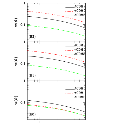
In this section we will first present results on the predicted angular correlation function $w(\theta)$ (see Figure 1) estimated for three different CDM spatially flat cosmological models taking into account the functional forms of the bias evolution (B0, B1, B2) introduced in the previous section. From figure 1, it is obvious that the amplitude of $w(\theta)$ increases for models with bias evolution in all cosmological models. This is to be expected due to the fact that the amplitude of the angular correlation function is affected by the expression $R(z)$, especially at high redshifts. Indeed, we observe that models with increasing bias as a function of redshift, give a stronger clustering signal (in small angular scales), relative to models with non-bias (B0). For the latter bias behaviour, it is interesting to see, that the predictions for $w(\theta)$ for the case of the $\tau$CDM and $\Lambda$CDM2 are almost the same.

Figure 1: Theoretical predictions of the angular correlation function $w(\theta)$.

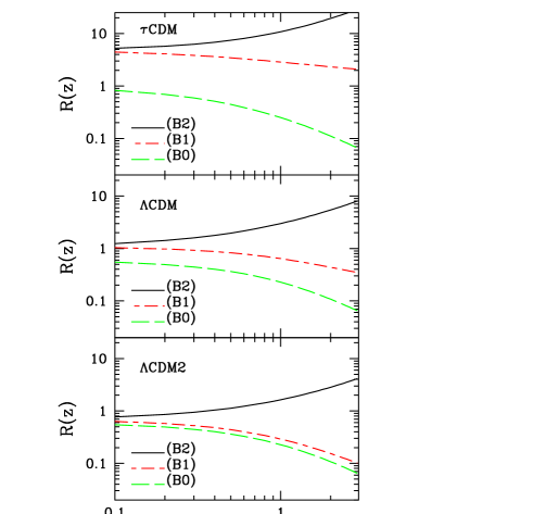
Therefore, in order to understand better the effects of AGN clustering, we present in figure 2 the quantity $R(z)=D^{2}(z)b^{2}(z)$ as a function of redshift for the three cosmological models, utilizing at the same time different bias evolution. It is quite obvious that the behaviour of the function $R(z)$ characterizes the clustering evolution with epoch. Figure 2, for example, clearly shows that the bias at high redshifts has different values in different cosmological models. In particular for the high $\sigma_{8}^{\rm mass}$ low-$\Omega_{\circ}$ flat model ($\Lambda$CDM2) the distribution of X-ray sources is only weakly biased, as opposed to the strongly biased distribution in the $\tau$CDM cosmological model.

Indeed the different functional forms of $b(z)$, provide clustering models where:

• AGN clustering is a decreasing function with redshift for (B0),

• AGN clustering is roughly constant for (B1). However, the $\Lambda$CDM2-B1 model gives lower $R(z)$ simply because the higher $\sigma_{8}^{\rm mass}$ normalization largely removes the clustering difference between the two other flat cosmological models with low $\sigma_{8}^{\rm mass}$ normalizations. In other words, the present bias value of the above model is almost $\sim 1$, which gives clustering behaviour similar to the $\Lambda$CDM2-B0.

• AGN clustering is a monotonically increasing function of redshift for (B2).

Figure 2: The function $R(z)=D^{2}(z)b^{2}(z)$ as a function of redshift, for different bias evolution models.

5 Application to the data

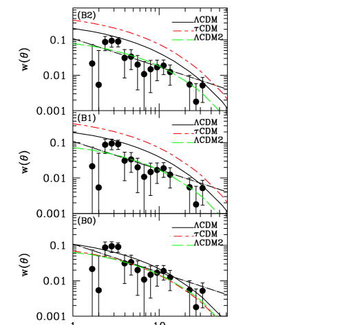
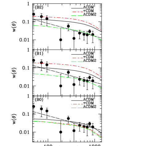
In Figure 3 we compare the angular correlation function of a sample of 2096 sources with a total sky coverage of 4.9sr detected in the ROSAT All-Sky Survey Bright Source Catalogue (see Akylas et al. 2000) with that predicted in various flat cosmological models. Considering a two point angular correlation function of the form $w(\theta)=(\theta/\theta_{\circ})^{1-\gamma}$, the above authors found $\theta_{\circ}=0.062^{\circ}$, $\gamma=1.8$ and spatial correlation length of $r_{\circ}\approx 6.5\pm 1.0h^{-1}$Mpc and $r_{\circ}\approx 6.7\pm 1.0h^{-1}$Mpc for stable and comoving clustering evolution respectively, similar to the optically selected AGN. Due to the fact that the above estimates have been focused on the local X-ray Universe, in this work we use complementary observational results from Vikhlinin & Forman (1995). They have analysed a set of deep ROSAT observations with a total sky coverage of 40 deg², in order to investigate the clustering properties of faint X-ray sources. Therefore, taking into account the correction for the amplification bias they claimed that the two point angular correlation function is well described by a power low with $\gamma=1.8$. Thus, in figure 4 we plot their results and the estimated angular correlation function for all nine models.

Figure 3: Comparison of the predicted angular correlation function for various cosmological models with that of the local AGN distribution, estimated by Akylas et al. (2000). Errorbars are determined by assuming Poisson statistics. The continuous dot-dash line represent the best fit to $w_{x}(\theta)$ derived by the above authors.

Figure 4: Comparison of the predicted angular correlation function for various models with that estimated by Vikhlinin & Forman (1995). The continuous dot-dash line represent the best fit to $w_{x}(\theta)$ derived by the above authors.

Table 2: $\chi^{2}$ probabilities (${\cal P}_{>\chi^{2}}^{B}$) of consistency between RASSBSC data and models.

Comparison Pair	${\cal P}_{>\chi^{2}}^{B}$
RASSBSC - $\Lambda$CDM-B0	0.81
RASSBSC - $\Lambda$CDM-B1	0.067
RASSBSC - $\Lambda$CDM-B2	0.019
RASSBSC - $\Lambda$CDM2-B0	0.19
RASSBSC - $\Lambda$CDM2-B1	0.42
RASSBSC - $\Lambda$CDM2-B2	0.57
RASSBSC - $\tau$CDM-B0	0.19
RASSBSC - $\tau$CDM-B1	2.88$\times 10^{-8}$
RASSBSC - $\tau$CDM-B2	3.00$\times 10^{-9}$

Table 3: $\chi^{2}$ probabilities (${\cal P}_{>\chi^{2}}^{F}$) of consistency between faint ROSAT data and models.

Comparison Pair	${\cal P}_{>\chi^{2}}^{F}$
faint ROSAT - $\Lambda$CDM-B0	0.037
faint ROSAT - $\Lambda$CDM-B1	3.67 $\times 10^{-4}$
faint ROSAT - $\Lambda$CDM-B2	1.72 $\times 10^{-6}$
faint ROSAT - $\Lambda$CDM2-B0	3.44 $\times 10^{-4}$
faint ROSAT - $\Lambda$CDM2-B1	3.21 $\times 10^{-3}$
faint ROSAT - $\Lambda$CDM2-B2	0.036
faint ROSAT - $\tau$CDM-B0	4.64 $\times 10^{-3}$
faint ROSAT - $\tau$CDM-B1	1.07$\times 10^{-12}$
faint ROSAT - $\tau$CDM-B2	4.73 $\times 10^{-15}$

In order to quantify the differences between models and data, we perform a standard $\chi^{2}$ test, for the bright (RASSBSC) and faint sources respectively, and we present the ${\cal P}_{>\chi^{2}}^{N}$ results in tables 2 and 3. Comparing the statistical results for both (a) high (faint sources) and (b) low (bright) redshift regimes, we can point out that for the bright X-ray sources the only models that are excluded by the data, at a relatively high significance level, are $\Lambda$CDM-B2, $\tau$CDM-B1 and $\tau$CDM-B2. Interestingly, for the faint objects the excluded models are $\Lambda$CDM-B1, $\Lambda$CDM-B2, $\Lambda$CDM2-B0, $\Lambda$CDM2-B1, $\tau$CDM-B0, $\tau$CDM-B1 and $\tau$CDM-B2. The above differences between the two kind of populations are to be expected simply because the cosmological evolution plays an important role on large scale structure clustering due to the fact that the high redshift objects are more biased tracers of the underlying matter distribution with respect to the low redshift objects (cf. Steidel et al. 1998). Also, from the faint X-ray sources results we would like to point out that there is not a single $\tau$CDM model that fits the data.

If we make the reasonable assumption that there is no correlation between the two X-ray populations, mostly due to the large distances involved, we can consider the RASSBSC and faint ROSAT catalogues as being independent of each other. Under this assumption the previous statistical tests can also be considered as independent. Indeed performing a standard Kolmogorov-Smirnov test comparing the two different spatial correlation functions, described by Akylas et al. (2000) and Vikhlinin & Forman (1995) we find that they are significantly different. In this framework the joint (overall) probability can be given by the following expression:

$$P={\cal P}_{>\chi^{2}}^{B}{\cal P}_{>\chi^{2}}^{F}\left[1-{\rm ln}({\cal P}_{>\chi^{2}}^{B}{\cal P}_{>\chi^{2}}^{F})\right]\;\;.$$ (15)

In table 4 we can see the corresponding joint probabilities for all our models. This overall statistical test proves that the $\Lambda$CDM-B0 and $\Lambda$CDM2-B2 models fit well the observational data at a relatively high significance level.

Table 4: The joint probabilities $P$.

Fitted Models	$P$
$\Lambda$CDM-B0	0.14
$\Lambda$CDM-B1	2.86 $\times 10^{-4}$
$\Lambda$CDM-B2	5.96 $\times 10^{-7}$
$\Lambda$CDM2-B0	7.00 $\times 10^{-4}$
$\Lambda$CDM2-B1	0.01
$\Lambda$CDM2-B2	0.10
$\tau$CDM-B0	7.08 $\times 10^{-3}$
$\tau$CDM-B1	1.41$\times 10^{-18}$
$\tau$CDM-B2	7.29$\times 10^{-22}$

Note that we have tested the AGN clustering predictions using also the SCDM (COBE normalized from Bunn & White 1997, with $h=0.5$, $\Gamma=0.5$ and $\sigma_{8}^{\rm mass}=1.22$) cosmological model and we found that it is excluded by the data at a high significance level (${\cal P}_{>\chi^{2}}^{B,F}\simeq 10^{-6}-10^{-9}$). Finally, a possible contamination of the AGN samples by stars, which can be assumed at first order to be distributed randomly on the sky, will lower the true amplitude of the AGN $w(\theta)$. We have crudely tested the effect on our model comparion results of an AGN amplitude drop of $\sim 10$% and found no qualitative differences whatsoever.

We should conclude that the behaviour of the observed angular correlation function of the X-ray sources is sensitive to the different cosmologies but at the same time there is a strong dependence on the bias models that we have considered in our analysis. By separating between low and high redshift regimes, we obtain results being consistent with the hierarchical clustering scenario, in which the AGN’s are strongly biased at all cosmic epochs (cf. Magliocchetti et al. 1999).

6 Conclusions

We have studied the clustering properties of the X-ray sources using the predicted angular correlation function for several cosmological models. We parametrize the predictions for $w(\theta)$ taking into account the behaviour of $b(z)$ for a non-bias model, a galaxy conserving bias model with $b(z)\propto(1+z)$ and for a galaxy merging bias model with $b(z)\propto(1+z)^{1.8}$. Utilising the measured angular correlation function, for faint and bright X-ray ROSAT sources, estimated in Vikhlinin & Forman (1995) and Akylas et al. (2000) respectively, we have compared them with the corresponding ones predicted in three cosmological models, namely the $\tau$CDM, $\Lambda$CDM and $\Lambda$CDM2 (with a high $\sigma_{8}^{\rm mass}$ value). We find that the models that best reproduce the observational results are:

• $\Lambda$CDM2 model ($\Omega_{\Lambda}=1-\Omega_{\circ}=0.7$) with high $\sigma_{8}^{\rm mass}=1.13$ and bias evolution described by $b(z)\propto(1+z)^{1.8}$.

• $\Lambda$CDM model ($\Omega_{\Lambda}=1-\Omega_{\circ}=0.7$) with low $\sigma_{8}^{\rm mass}=0.9$ and bias evolution by $b(z)\equiv 1$.

References

- [] Akylas, A., Georgantopoulos, I., Plionis, M., 2000, MNRAS, 318, 1036
- [] Bagla J. S. 1998, MNRAS, 299, 424
- [] Bardeen, J.M., Bond, J.R., Kaiser, N. & Szalay, A.S., 1986, ApJ, 304, 15
- [] Basilakos S., & Plionis, M., 2001, ApJ, in press
- [] Benson, A. J., Cole, S., Frenk, S. C., Baugh, M. C., & Lacey, G. C., 2000, MNRAS, 311, 793
- [] Boyle, B. J., Griffiths, R. E., Shanks, T., Stewart, G. C., Georgantopoulos, I., 1993, MNRAS, 260, 49
- [] Boyle, B. J., & Mo, H. J., 1993, MNRAS, 260, 925
- [] Bunn, E. F., White, M., 1997, ApJ, 480, 6
- [] Catelan, P., Lucchin, F., Mataresse, S. & Porciani, C., 1998, MNRAS, 297, 692
- [] Carrera, F. J., Barcons, X., Fabian, A. C., Hasinger, G., Mason, K. O., McMahon, R. G., Mittaz, J. P. D., Page, M. J., 1998, MNRAS, 299, 229
- [] Georgantopoulos, I., Stewart, G. C., Shanks, T., Boyle, B J., Griffiths, R. E., 1996, MNRAS, 280, 276
- [] Cole, S., Hatton, S., Weinberg, D. H., Frenk, C. S., 1998, MNRAS, 300, 945
- [] Croom, S. M., & Shanks, T., 1996, MNRAS, 281, 893
- [] Dekel, A., & Lahav, O., 1999, ApJ, 520, 24
- [] Eke, V., Cole, S., Frenk, C. S., 1996, MNRAS, 282, 263
- [] Fry, J.N., 1996, ApJ, 461, 65
- [] Hartwick, F. D. A., Schade, D., 1989, ARA&A, 28, 437
- [] Kaiser, N., 1984, ApJ, 284, L9
- [] La Franca F., Andreani, P., Cristiani, S., 1998, ApJ, 497, 529
- [] Maddox, S., Efstathiou, G., Sutherland, W. J., Loveday, J., 1990, MNRAS, 242, 457
- [] Magliocchetti, M., Maddox, S. J., Lahav, O., Wall, J. V., 1999, MNRAS, 306, 943
- [] Magliocchetti, M., Bagla, J. S., Maddox, S. J., Lahav, O., 2000, MNRAS, 314, 546
- [] Martini, P., & Weinberg, D. H., 2000, ApJ, 547, 12
- [] Mason, K. O., et al., 2000, MNRAS, 311, 456
- [] Matarrese, S., Coles, P., Lucchin, F., Moscardini, L., 1997, MNRAS, 286, 115
- [] Mo, H.J, & White, S.D.M 1996, MNRAS, 282, 347
- [] Moscardini, L., Coles, P., Lucchin, F., Matarrese, S., 1998, MNRAS, 299, 95
- [] Nusser, A. & Davis, M., 1994, ApJ, 421, L1
- [] Peacock, J. A., Dodds, S. J., 1994, MNRAS, 267, 1020
- [] Peebles P.J.E., 1980, The Large-Scale Structure of the Universe, Princeton University Press, Princeton New Jersey
- [] Peebles P.J.E., 1993, Principles of Physical Cosmology, Princeton University Press, Princeton New Jersey
- [] Perlmutter, S., et al., 1999, ApJ, 517, 565
- [] Riess, A. G., et al., 1998, AJ, 116, 1009
- [] Shanks, T., & Boyle, B. J., 1994, MNRAS, 271, 753
- [] Steidel, C.C., Adelberger, L.K., Dickinson, M., Giavalisko, M., Pettini, M., Kellogg, M., 1998, ApJ, 492, 428
- [] Sugiyama, N., 1995, ApJS, 100, 281
- [] Tegmark, M. & Peebles, P.J.E, 1998, ApJ, 500, L79
- [] Vikhlinin, A. & Forman, W., 1995, ApJ, 455, 109