Generating non-Gaussian maps with a given power spectrum and bispectrum

Abstract

We propose two methods for generating non-Gaussian maps with fixed power spectrum and bispectrum. The first makes use of a recently proposed rigorous, non-perturbative, Bayesian framework for generating non-Gaussian distributions. The second uses a simple superposition of Gaussian distributions. The former is best suited for generating mildly non-Gaussian maps, and we discuss in detail the limitations of this method. The latter is better suited for the opposite situation, i.e. generating strongly non-Gaussian maps. The ensembles produced are isotropic and the power spectrum can be jointly fixed; however we cannot set to zero all other higher order cumulants (an unavoidable mathematical obstruction). We briefly quantify the leakage into higher order moments present in our method. We finally present an implementation of our code within the HEALPIX package [1].

I Introduction

In most inflationary scenarios the fluctuations in the matter fields generated by the oscillating inflaton display Gaussian statistics. This requires the temperature fluctuations in the Cosmic Microwave Background (CMB) to be Gaussian distributed to a very high degree of accuracy at sufficiently large angular scales. On smaller scales the effect of late time non-linear evolution will introduce a certain amount of non-Gaussianity in the CMB. The study of the non-Gaussianity of CMB fluctuations is therefore crucial to both the understanding of the fundamental processes generating the fluctuations and to the understanding of the various foreground and astrophysical contributions.

In addressing an issue of this nature with reference to observational strategies it is important to be able to simulate CMB maps with non-Gaussian signatures. These can then be used in the refinement of estimation techniques and the design of evermore accurate satellite, balloon-borne, and ground-based experiments. It seems therefore desirable to develop fast algorithms for simulating not only Gaussian signals (as extensively done in the past, e.g.[1]), but also maps allowing for non-Gaussianity. In the past the bispectrum has proved an invaluable tool in studying CMB non-Gaussianity (see for instance [2, 3, 4, 5, 6, 7]). Also algorithms generating Gaussian maps usually use the power spectrum as a controlling parameter. We therefore seek to complement earlier work by producing an algorithm for generating non-Gaussian maps with fixed power spectrum and bispectrum. As a matter of fact the algorithm we shall propose can be extended to fix simultaneously any higher order moment, naturally at a computational cost.

The difficulty in generating non-Gaussian maps is in part due to the lack of suitable Probability Distribution Functions (PDFs) with the required parametrisation, and in part due to the requirement that non-zero higher moments require the multivariate generation of correlated sets of modes. The latter is imposed by statistical isotropy, in all cases except in Gaussian maps. We shall address the first of these problems with reference to the recent work in [7], in which a rigorous, non-perturbative, Bayesian framework for generating non-Gaussian distributions was proposed. We also propose an alternative PDF, a simple superposition of Gaussian distributions. We then address the second problem with a rather simple trick for creating the required mode correlations enforcing isotropy.

This paper is organised as follows. In section II we introduce two exact, non-perturbative univariate distributions which produce non-Gaussian ensembles with fixed variance and skewness. In section III we derive the higher moments for both distributions. Section IV shows how we can employ the non-Gaussian 1-D distributions to generate isotropic ensembles of non-Gaussian maps with given angular power spectra and bispectra. We show examples of such distributions in section V and discuss the results and applications of this work section VI.

II Exact non-Gaussian 1-D distributions

In this section we introduce two classes of distributions which can be employed to generate random numbers with exactly specified second and third moments. The first was introduced as a non-perturbative, non-Gaussian likelihood in the Bayesian analysis of the CAT/VSA data [7]. It was originally introduced, in a theoretical context, in the study of off-the-ground state perturbations in the inflaton field[8]. The second class of distributions is an ad hoc solution obtained by requiring the simplest superposition of Gaussian PDFs that results in a distribution with a given second and third moments.

Both PDF functions can be used to generate distributions with fixed power spectra and bispectra (and optionally higher order spectra). The first is best suited for mild non-Gaussianity; the latter for strong departures from Gaussianity.

A The non-perturbative harmonic likelihood

We now summarise the method of Rocha et al. [7, 9]. Let $x$ represent a general random variable. We build its distribution from the space of wave-functions which are energy eigenmodes of a linear harmonic oscillator (see e.g [10]). We have that

$$\psi(x)=\sum\alpha_{n}\psi_{n}(x),$$ (1)

where $n$ labels the energy spectrum $E_{n}=\hbar\omega(n+1/2)$, and

$$\psi_{n}(x)=C_{n}H_{n}{\left(x\over{\sqrt{2}}\sigma_{0}\right)}e^{-{x^{2}\over 4\sigma_{0}^{2}}},$$ (2)

with normalisation fixing $C_{n}$ as

$$C_{n}={1\over(2^{n}n!{\sqrt{2\pi}}\sigma_{0})^{1/2}}\,.$$ (3)

The only constraint upon the amplitudes $\alpha_{n}$ is

$$\sum|\alpha_{n}|^{2}=1,$$ (4)

which can be eliminated explicitly by imposing the condition

$$\alpha_{0}=\sqrt{1-\sum_{1}^{\infty}|\alpha_{n}|^{2}}.$$ (5)

$\sigma_{0}^{2}$ is the variance associated with the (Gaussian) probability distribution for the ground state $|\psi_{0}|^{2}$. We define Hermite polynomials $H_{n}(x)$ as

$$H_{n}(x)=(-1)^{n}e^{x^{2}}\frac{d^{x}}{dx^{n}}e^{-x^{2}},$$ (6)

with normalisation

$$\int^{\infty}_{-\infty}e^{-x^{2}}H_{n}(x)H_{m}(x)dx=2^{n}\pi^{1/2}n!\delta_{nm}.$$ (7)

The most general probability density is thus:

$$P=|\psi|^{2}={e^{-{x^{2}\over 2\sigma_{0}^{2}}}\over{\sqrt{2\pi}}}|\alpha_{n}C_{n}H_{n}{\left(x\over{\sqrt{2}}\sigma_{0}\right)}|^{2}$$ (8)

The ground state (or “zero-point”) fluctuations are Gaussian, but any admixture with other states will be reflected in a non-Gaussian distribution function.

It can be shown [9, 7] that the $\alpha_{n}$ reduce to the cumulants $\kappa_{n}$ (up to a multiplicative constant) for mild, “perturbative”, non-Gaussianity. This is achieved by reducing the probability density (8) to an asymptotic expansion around the Gaussian distribution function (the so-called Edgeworth expansion). Such asymptotic expansions on the space of orthonormal Hermite polynomials suffer from the fact that truncations at a finite order of cumulants lead to pseudo-distributions which are not positive definite. This is not the case here and the advantage of using the $\alpha_{n}$ over cumulants is that setting all but a finite number of them to zero still leads to proper distributions. In some sense the $\alpha_{n}$ are non-perturbative generalizations of cumulants.

The above probability density may be easily applied to generate a centered distribution with a fixed variance and skewness. Let us start with the PDF

$$P(x)=\frac{\exp(-x^{2}/2\sigma^{2})}{\sqrt{2\pi}\sigma}\left[\alpha_{0}+\frac{\alpha_{1}}{\sqrt{2}}H_{1}\left(\frac{x}{\sqrt{2}\sigma}\right)+\frac{\alpha_{2}}{\sqrt{8}}H_{2}\left(\frac{x}{\sqrt{2}\sigma}\right)+\frac{\alpha_{3}}{\sqrt{48}}H_{3}\left(\frac{x}{\sqrt{2}\sigma}\right)\right]^{2},$$ (9)

in which all the $\alpha_{n}$ are real and we have set all $\alpha_{n}=0$ for $n>3$. We then calculate moments around the origin defined as

$$\mu_{n}=\langle x^{n}\rangle=\int^{\infty}_{-\infty}x^{n}P(x)dx.$$ (10)

For a normalised density we have $\mu_{0}=\alpha_{0}^{2}+\alpha_{1}^{2}+\alpha_{2}^{2}+\alpha_{3}^{2}=1$ and the first three moments given by

$$\mu_{1} = (2\sigma^{2})^{1/2}\left(2\alpha_{1}\alpha_{2}+\sqrt{2}\alpha_{0}\alpha_{1}+\sqrt{6}\alpha_{2}\alpha_{3}\right),$$ (11)

$$\mu_{2} = \sigma^{2}\left(\alpha_{0}^{2}+3\alpha_{1}^{2}+5\alpha_{2}^{2}+7\alpha_{3}^{2}+2\sqrt{2}\alpha_{0}\alpha_{2}+2\sqrt{6}\alpha_{1}\alpha_{3}\right),$$ (12)

$$\mu_{3} = (2\sigma^{2})^{3/2}\left(\frac{3}{\sqrt{2}}\alpha_{0}\alpha_{1}+6\alpha_{1}\alpha_{2}+\frac{9\sqrt{3}}{\sqrt{2}}\alpha_{2}\alpha_{3}+\sqrt{3}\alpha_{0}\alpha_{3}\right).$$ (13)

The aim is to have a centered distribution with $\mu_{1}=0$. This can be achieved by setting $\alpha_{1}=0$ and $\alpha_{2}=0$ in which case we are left with the system

$$1 = \alpha_{0}^{2}+\alpha_{3}^{2},$$ (14)

$$\mu_{2} = {\sigma^{2}}\left(\alpha_{0}^{2}+7\alpha_{3}^{2}\right),$$ (15)

$$\mu_{3} = (2\sigma^{2})^{3/2}\sqrt{3}\alpha_{0}\alpha_{3}.$$ (16)

Setting $\alpha_{0}=\sqrt{1-\alpha_{3}^{2}}$, we then solve for $\sigma$ and $\alpha_{3}$ for particular values of the required second and third moments $\mu_{2}$ and $\mu_{3}$

$$\sigma^{3} = \frac{\mu_{3}}{2\sqrt{6}(1-\alpha_{3}^{2})^{1/2}\alpha_{3}},$$ (17)

$$\alpha_{3}^{2} = \frac{1}{6}\left(\frac{\mu_{2}}{\sigma^{2}}-1\right).$$ (18)

a problem we deal with numerically. Hence we arrive at a 1-D centered distribution with fixed variance and skewness.

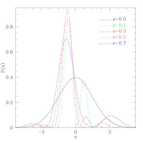
By restricting ourselves to only two parameters we have in fact constrained the space of possible distribution functions. This is reflected in the fact that we cannot generate distributions with any given variance and skewness. By studying the function for the relative skewness $s$

$$s\equiv{\mu_{3}\over\mu_{2}^{3/2}}={2\sqrt{6}(1-\alpha_{3}^{2})\alpha_{3}\over(1+6\alpha_{3}^{2})^{3/2}}$$ (19)

it is easy to see that the maximal relative skewness is

$$s=\pm 0.739\ \ \ \ \mbox{at}\ \ \ \ \alpha_{3}=\pm 0.278.$$ (20)

In general our method can generate higher values of $s$ (since it can generate any distribution), but for that purpose one needs more parameters $\alpha_{n}$. The generalization of the above construction for more parameters is trivial if somewhat tedious.

FIG. 1.: The left panel shows the distribution $P(x)$ for various values for the relative skewness parameter $s=\mu_{3}/\mu_{2}^{3/2}$ ($0.0\leq s\leq 0.7$) . The right panel shows the distribution $T(x)$ for $0.0\leq s\leq 10.0$.

B A tailor made distribution function

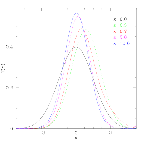
One way to overcome the limitations of the distribution described above without increasing the number of parameters is to build a distribution by ‘summing’ Gaussians. In fact it is obvious that the distribution $P(x)$ can be well approximated by a series of uncentered Gaussian functions of different heights and widths. Consider, for example, the distribution obtained by the superposition of three Gaussian distributions

$$T(x)=\frac{1}{(2+\beta_{0})\sqrt{\pi}}\left(e^{-x^{2}}+e^{-(x-\beta_{0}\beta_{1})^{2}}+\beta_{0}e^{-(x+\beta_{1})^{2}}\right).$$ (21)

In this case the first three moments of the distribution are given by

$$\mu_{1} = 0,$$ (22)

$$\mu_{2} = \frac{1}{2(2+\beta_{0})}\left(2+\beta_{0}+2\beta_{0}\beta_{1}^{2}(1+\beta_{0})\right),$$ (23)

$$\mu_{3} = \frac{\beta_{0}\beta_{1}^{3}(\beta_{0}^{2}-1)}{2+\beta_{0}}.$$ (24)

In contrast to the previous distribution the value of $s$ is now effectively unconstrained. In practice we find that in this case the range of $s$ is limited only by numerical effects in the random number generation process.

Fig. 1 compares the distributions $P(x)$ and $T(x)$ for various values of the relative skewness $s$. The former may be considered somewhat ‘unphysical’ since the minima in the functions will tend to produce ‘holes’ in the distribution of variates for each particular set of moments (this is not surprising since the PDF originates from the wavefunction of an oscillator). We should point out though that the present exercise is aimed at producing maps for the sole purpose of testing statistical tools and not to reproduce theoretically motivated models of the cosmic microwave backgrounds. The adaptation of the method to more suitably physical non-Gaussian distribution functions such as the PDF $T(x)$ above is trivial as we have shown.

A word of caution is in order, concerning the numerical aspects of generating univariate random numbers with a given non-Gaussian PDF. The Jacobian required to generate the random variables using the transformation method is not easily computable in the case of the PDFs $P(x)$ and $T(x)$. We advocate, instead, the use of the well known rejection method [11] to generate the required one dimensional random variables.

III Leakage into the higher moments

Both distributions have general solutions for all higher order moments $\mu_{n}$. The fourth and sixth order moments are of particular interest since they generate the sample variance and hence the cosmic variance in the observed power spectrum and bispectrum of the realisations. For $n$ even we find the following relatively simple expressions for the moments

$$\mu_{n}=\frac{(2\sigma)^{n}}{\sqrt{\pi}}\left[\alpha_{0}^{2}\Gamma\left(\frac{1+n}{2}\right)+\alpha_{3}^{2}\left\{3\Gamma\left(\frac{3+n}{2}\right)-4\Gamma\left(\frac{5+n}{2}\right)+\frac{4}{3}\Gamma\left(\frac{7+n}{2}\right)\right\}\right],$$ (25)

for the distribution $P(x)$ and

$$\mu_{n}=\frac{\Gamma\left(\frac{1+n}{2}\right)}{(2+\beta_{0})\sqrt{\pi}}\left[e^{-\beta_{1}^{2}}\beta_{0}M\left(\frac{1+n}{2},\frac{1}{2},\beta_{1}^{2}\right)+e^{-\beta_{0}^{2}\beta_{1}^{2}}M\left(\frac{1+n}{2},\frac{1}{2},\beta_{0}^{2}\beta_{1}^{2}\right)+1\right],$$ (26)

for the distribution $T(x)$ where $M(a,b,c)$ are the confluent hypergeometric functions [19]. Unfortunately the non-linear dependence of the parameters $\sigma,\alpha_{n}$ and $\beta_{n}$ on the required ensemble moments complicates the analytical form for the sample variances $\sigma^{2}(\mu_{2})$ and $\sigma^{2}(\mu_{3})$. In practice therefore the sample variances would be calculated numerically via the above expressions and making use of the solutions to the systems (14) and (22) or via Monte-Carlo simulations.

IV Generating non-Gaussian maps with fixed angular power spectrum and bispectrum

We now propose to apply this method to the generation of non-Gaussian maps with fixed angular power spectrum $C_{\ell}$ and bispectrum $B_{\ell}$. The broader context is the generation of non-Gaussian signals to be be used in simulations of upcoming satellite experiments.

The distributions of the previous section have the disadvantage that they can only generate non-Gaussian 1-D distributions. As a result, when a likelihood constructed using $P(x)$ is applied to CMB maps as in Rocha et al., it probes a combination of non-Gaussianity and anisotropy. Consider, for instance, the generation of a full-sky map with temperature fluctuations $\frac{\Delta T}{T}({\bf n})$, by means of its spherical harmonic components:

$$\frac{\Delta T}{T}({\bf n})=\sum_{\ell m}a_{\ell m}Y_{\ell m}({\bf n}).$$ (27)

If we set $\alpha_{3}\neq 0$ in the above distribution and use it to generate a set of $\Re(a_{\ell 0})$ we will have $\langle(\Re a_{\ell 0})^{3}\rangle\neq 0$, with $\langle(\Re a_{\ell m})^{3}\rangle=0$ for $m\neq 0$. Isotropy, on the other hand, imposes “selection rules” upon correlators, in this case

$${\langle a_{\ell_{1}m_{1}}a_{\ell_{2}m_{2}}a_{\ell_{3}m_{3}}\rangle}=\left(\begin{array}[]{ccc}\ell_{1}&\ell_{2}&\ell_{3}\\ m_{1}&m_{2}&m_{3}\end{array}\right)B_{\ell_{1}\ell_{2}\ell_{3}},$$ (30)

where the quantity $(\ldots)$ is the Wigner $3J$ symbol, and the coefficients $B_{\ell_{1}\ell_{2}\ell_{3}}$ are the bispectrum (abbreviated to $B_{\ell}$ for the case $\ell_{1}=\ell_{2}=\ell_{3}$). Hence the distribution we have just generated is not only non-Gaussian but also automatically anisotropic since all third order correlators except for $\langle a_{\ell 0}\rangle$ are zero.

If we are to impose isotropy, we must necessarily have correlated $a_{\ell m}$, a feature not allowed by the method of Rocha et al. In the present context a correlated set of $a_{\ell m}$ is equivalent to a series of coupled harmonic oscillators. The obvious way to achieve the necessary correlations would be to use the Hilbert space of coupled harmonic oscillators to set up the most general multi-variate distribution but this proves to be impractical. Here we introduce a simple but crucial modification which restores isotropy.

We propose to set up an isotropic ensemble in two steps. First we generate an anisotropic ensemble by drawing all $a_{\ell m}$ from a Gaussian distribution with variance spectrum $C_{\ell}$, except for the $m=0$ mode. The latter is given one of the PDFs described in the previous section, with variance $C_{\ell}$ and skewness

$$s_{\ell}=\left(\begin{array}[]{ccc}\ell&\ell&\ell\\ 0&0&0\end{array}\right)^{-1}B_{\ell}$$ (31)

The appropriate PDF is enforced using the rejection method, as described above. For each set of $C_{\ell}$ and $B_{\ell}$ we solve the systems given by Eqs. (14) or (22) numerically to obtained the required values for the parameters $\sigma$, $\alpha_{0}$ and $\alpha_{3}$ or $\beta_{0}$ and $\beta_{1}$ . We label the resulting ensemble $a$, for anisotropic.

We then apply a random rotation to each realization in the ensemble $a$, with a uniform distribution of Euler angles. In this way we arrive at an isotropic ensemble of temperature maps, labelled by $i$, with spherical harmonic coefficients

$$b^{\ell}_{m}=\sum_{m^{\prime}}{\cal D}^{\ell}_{mm^{\prime}}(\Omega)a^{\ell}_{m^{\prime}}$$ (32)

where ${\cal D}^{\ell}_{mm^{\prime}}$ is the rotation matrix, and $\Omega$ denote the 3 Euler angles. The 2-point correlators are

$${\langle b_{\ell_{1}m_{1}}b^{\star}_{\ell_{2}m_{2}}\rangle}_{i}=\sum_{m_{1}^{\prime}m_{2}^{\prime}}{\langle{\cal D}^{\ell_{1}}_{m_{1}m_{1}^{\prime}}(\Omega){\cal D}^{\ell_{2}\star}_{m_{2}m_{2}^{\prime}}(\Omega)\rangle}_{\Omega}{\langle a_{\ell_{1}m_{1}^{\prime}}a^{\star}_{\ell_{2}m_{2}^{\prime}}\rangle}_{a}=\delta_{\ell_{1}\ell_{2}}\delta_{m_{1}m_{2}}C_{\ell_{1}},$$ (33)

hence we have $C_{\ell}^{i}\equiv C_{\ell}^{a}$.

The 3-point correlators are zero for any correlator involving different $\ell$. However we now have

$${\langle b_{\ell m_{1}}b_{\ell m_{2}}b_{\ell m_{3}}\rangle}_{i} = \sum_{m_{1}^{\prime}m_{2}^{\prime}m_{3}^{\prime}}{\langle{\cal D}^{\ell}_{m_{1}m_{1}^{\prime}}(\Omega){\cal D}^{\ell}_{m_{2}m_{2}^{\prime}}(\Omega){\cal D}^{\ell}_{m_{3}m_{3}^{\prime}}(\Omega)\rangle}_{\Omega}{\langle a_{\ell m_{1}^{\prime}}a_{\ell m_{2}^{\prime}}a_{\ell m_{3}^{\prime}}\rangle}_{a}$$ (34)

$$= {\langle{\cal D}^{\ell}_{m_{1}0}(\Omega){\cal D}^{\ell}_{m_{2}0}(\Omega){\cal D}^{\ell}_{m_{3}0}(\Omega)\rangle}_{\Omega}\times s_{\ell}$$ (35)

$$= {\langle Y^{\ell}_{m_{1}}(\Omega)Y^{\ell}_{m_{2}}(\Omega)Y^{\ell}_{m_{3}}(\Omega)\rangle}_{\Omega}\times s_{\ell}$$ (36)

$$= {\left(\begin{array}[]{ccc}\ell&\ell&\ell\\ 0&0&0\end{array}\right)}{\left(\begin{array}[]{ccc}\ell&\ell&\ell\\ m_{1}&m_{2}&m_{3}\end{array}\right)}s_{\ell}$$ (41)

$$= {\left(\begin{array}[]{ccc}\ell&\ell&\ell\\ m_{1}&m_{2}&m_{3}\end{array}\right)}B_{\ell}$$ (44)

(note that with one index $m$ set to zero the rotation matrices reduce to spherical harmonics, one of the Euler angles becoming irrelevant). Again we have recovered the original bispectrum with $B_{\ell}^{i}\equiv B_{\ell}^{a}$.

Hence the procedure we have defined produces the desired isotropic ensemble with a fixed angular power spectrum and bispectrum. The random rotations produce the necessary correlations between the $a_{\ell m}$ coefficients to ensure isotropy. However, by means of this procedure, we are unable to generate maps with non vanishing inter-$\ell$ bispectrum coefficients (as studied in [3, 4, 5, 6]).

Note that we can also draw all $a_{\ell m}$ from the 1-D PDFs introduced above, and then subject them to a random rotation. The argument presented here still goes through, and an isotropic ensemble is still obtained. However, as we shall see later, the cosmic variance in the estimators for the $C_{\ell}$ and $B_{\ell}$ will be larger in this case.

V Simulated non-Gaussian maps

We now present CMB temperature maps using the prescriptions detailed in the previous sections. We generate full sky maps pixelised using the HEALPIX [1] package at pixelisation levels $128$ and $512$, equivalent to $196,608$ and $3,145,728$ pixels respectively. We generate maps which include a cosmological signal in the form of a standard $\Lambda$CDM power spectrum computed using CMBFAST [17] and finite beam sizes. Instrument specific noise and physically motivated profiles for the bispectrum will be treated in further work [15].

For simplicity we shall assume a bispectrum which is fixed relative to the power spectrum (i.e. $B_{\ell}=sC_{\ell}^{3/2}$) with a ratio which is the same for all scales (i.e. with $s_{\ell}\equiv s$ constant). This is a rather artificial asumption since in practice the host of non-linear, secondary and foreground contributions to the CMB [16] and possible primordial non-Gaussianity will arise at different angular scales. Theoretically motivated bispectra and the addition of instrument specific noise will be discussed in further work [15], and are straightforward to obtain with our method at no extra computational cost. We use both the PDFs discussed above to generate the 1-D distributions required for the production of the initial anisotropic ensembles.

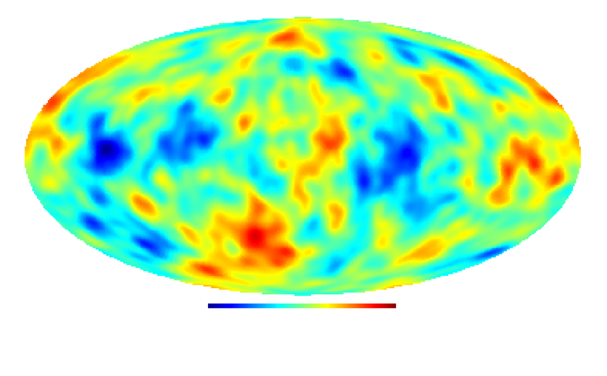
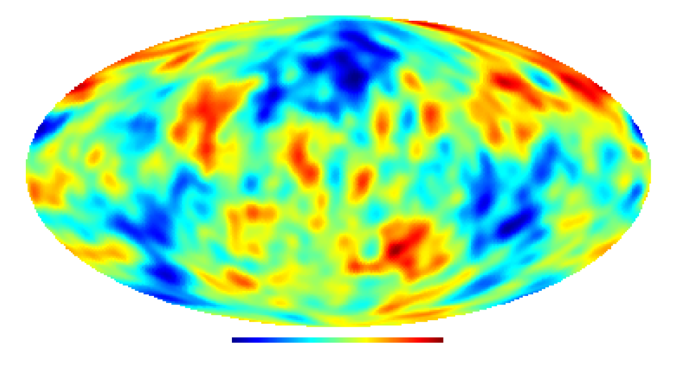
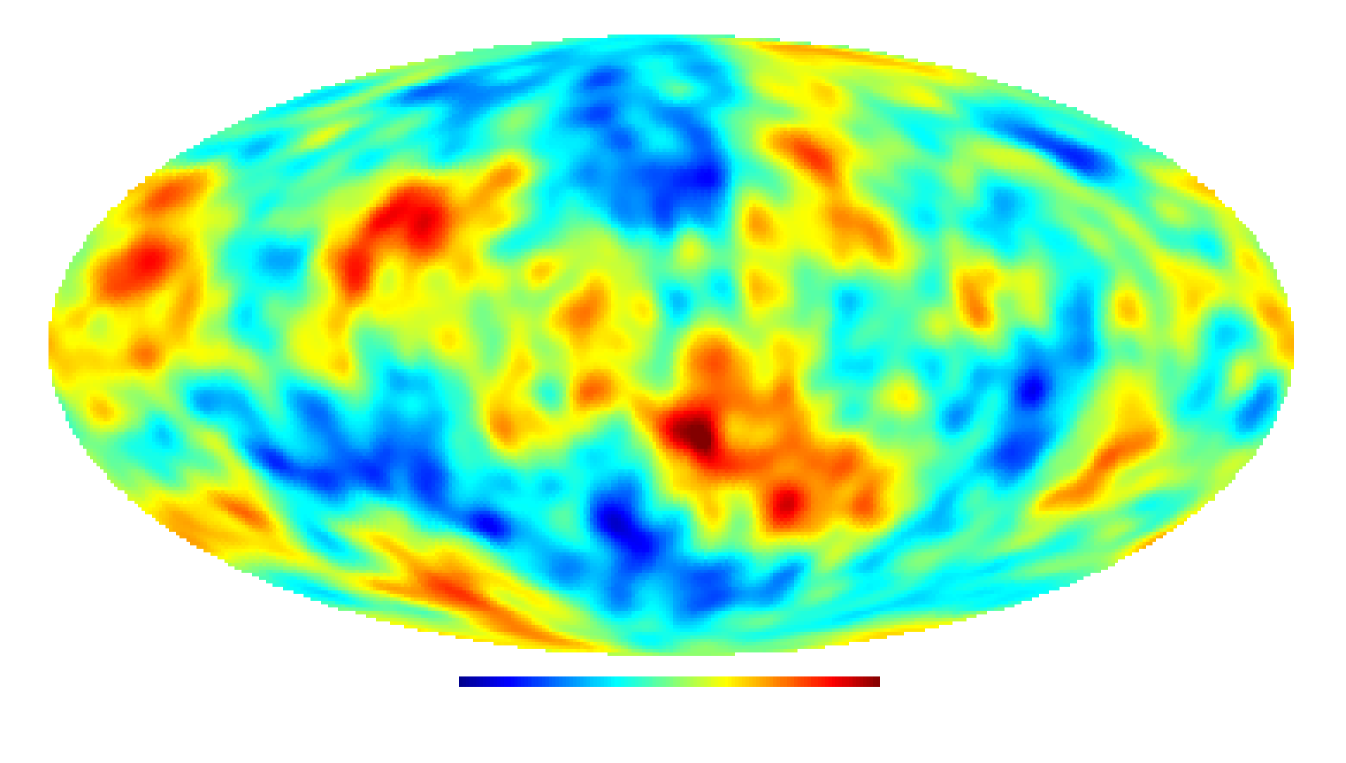
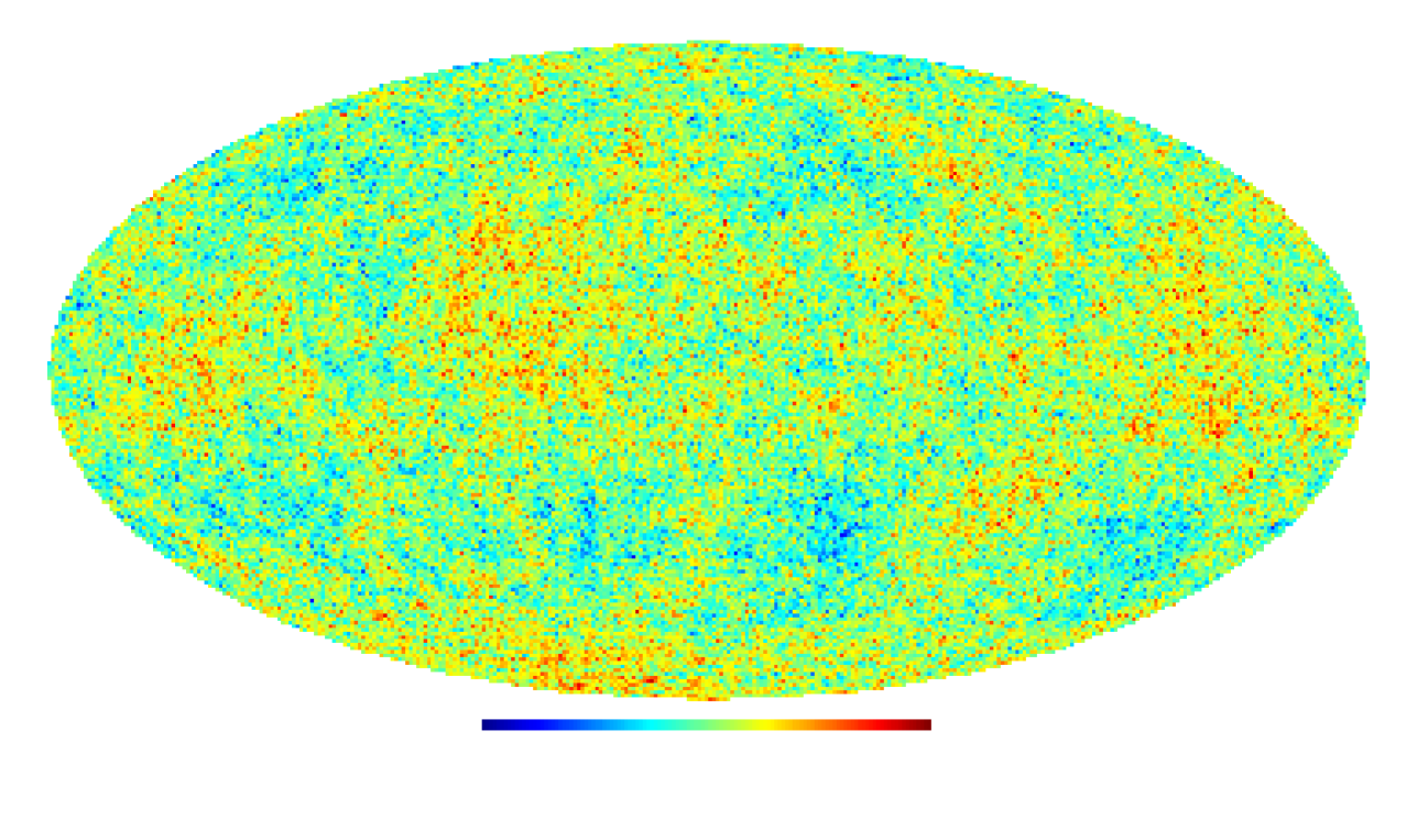
In Fig. 2 we show a Gaussian realisation of a standard $\Lambda$CDM model at COBE-DMR [20] resolution. The equivalent non-Gaussian realisations with the same power spectrum are shown in Figs. 3 and 4 which are generated using the PDF $T(x)$ and values for the parameter $s$ of $0.5$ and $2.0$ respectively. Fig. 5 shows a non-Gaussian realisation ($s=2.0$) with the same power spectrum and MAP [21] resolution.

FIG. 2.: HEALPIX map of a noiseless, Gaussian CMB realisation at COBE beam resolution (normalised temperature units). The map was generated using a standard $\Lambda$CDM power spectrum ($\Omega_{\Lambda}=0.7$, $\Omega_{CDM}=0.25$, $\Omega_{b}=0.05$, $h=0.7$ and $n_{s}=1.0$).

FIG. 3.: A non-Gaussian realisation at the same resolution generated with the same $\Lambda$CDM power spectrum and a ‘white’ bispectrum with $s=0.5$. The PDF $T(x)$ was used as the non-Gaussian generator.

FIG. 4.: A similar realisation with $s=2.0$.

FIG. 5.: Same as above but at the resolution of the MAP experiment.

We first make use of our maps to examine possible effects of non-Gaussianity upon estimation of the power spectrum. For this purpose we compare the observed power

$$C_{\ell}^{obs}=\frac{1}{2\ell+1}\sum_{m=-\ell}^{\ell}|a^{\ell 2}_{m}|,$$ (45)

in the non-Gaussian ensembles with that of the usual Gaussian ensembles. Different PDFs will produce ensembles with different cosmic variances (for the power) and in particular the cosmic variance will be different from that of Gaussian ensembles. Assuming the $a_{m}^{\ell}$ modes to be Gaussian distributed the power spectrum will have a $\chi_{2\ell+1}^{2}$ distribution which yields a particularly simple sample variance

$$\sigma^{2}(C^{obs}_{\ell})=\frac{2C^{2}_{\ell}}{(2\ell+1)},$$ (46)

for zero noise and infinitely thin beam (see e.g. [12, 18]). In the non-Gaussian case the variance will assume a more complicated form due to a non-zero contribution from the fourth order cumulant (or connected moments in analogy to the connected Green’s functions of field theory):

$$\sigma^{2}(\mu_{2})=\kappa_{4}+2\mu^{2}.$$ (47)

In many motivated examples non-Gaussian processes display higher cosmic variance in the power; an example is texture models as studied in [22].

FIG. 6.: The estimated power spectrum for ensembles of $10$ pure signal maps. The solid line is the power spectrum of a standard $\Lambda$CDM model ($\Omega_{\Lambda}=0.7$, $\Omega_{CDM}=0.25$, $\Omega_{b}=0.05$, $h=0.7$ and $n_{s}=1.0$). The dotted lines show the extent of cosmic variance of the averaged power for the respective Gaussian ensemble. The short dashed line is for an ensemble generated using the distribution $P(x)$ with $s=0.5$. The short dashed dotted line is for $s=0.5$ but generated using $T(x)$ and the long dashed dotted line is for $T(x)$ with $s=5.0$. The ensembles in the left panel were generated using only the $a_{\ell 0}$ modes as the non-Gaussian seeds in the original anisotropic, uncorrelated ensembles whereas in the right panel all the modes were originally non-Gaussian.

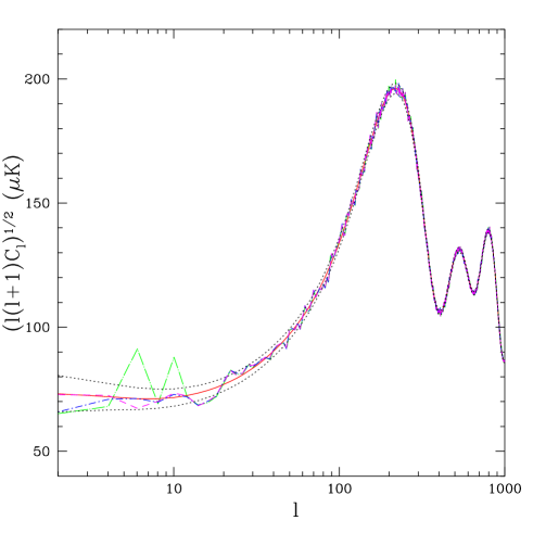
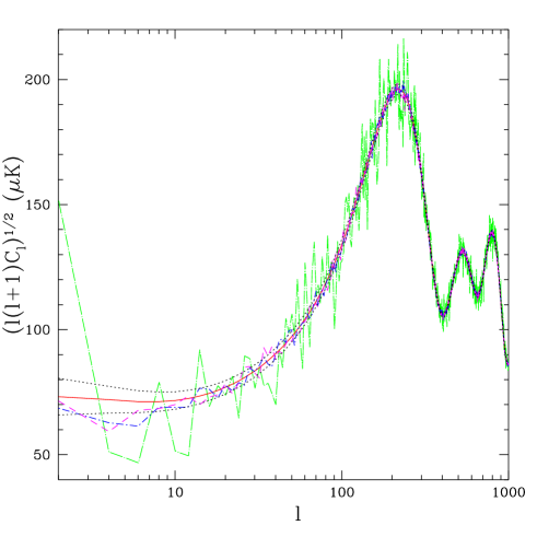
In Fig. 6 we show the average power spectrum for an ensemble of $10$ maps for mild and extreme values for the relative skewness parameter $s$. The maps do not include any noise contribution or beam effects. The right panel shows the average power for maps where all $a_{\ell m}$ modes are non-Gaussian in the original anisotropic, uncorrelated ensemble. The left panel instead is for the case where only the $a_{\ell 0}$ of the original modes are non-Gaussian. The dotted line shows the extent of the $1$-sigma cosmic variance for an equivalent Gaussian ensemble.

We see that the sample variance of the power for the non-Gaussian variables is comparable to that of its Gaussian counterpart for low $s$ and grows for larger value of the relative skewness. This dependence is expected since we know that $\kappa_{4}(\sigma,\alpha_{0},\alpha_{3})\equiv\kappa_{4}(s,C_{\ell})$. Note that the isotropising rotation does not affect ensemble averages, so that the sample variances of estimators in the isotropic ensemble trace the variances of the 1-D distributions generating the non-Gaussianity. In general the contribution from the connected moments can be derived analytically since they can be expanded in a series of moments [18]. In this case though the solution for $\sigma(\mu_{2})$ in terms of $C_{\ell}$ is very contrived and has no simple expression as the one above for the Gaussian case. Numerically estimation on a case by case basis will give a more feasible determination of the sample variance of the estimators being used.

We now turn to the issue of the detectability of non-Gaussian bispectra making use of our maps. In Figs. 7 and 8 we show the distribution of the value for the observed bispectrum [2]

$$B^{obs}_{\ell}=\sum_{m_{1}m_{2}m_{3}}{\left(\begin{array}[]{ccc}\ell&\ell&\ell\\ m_{1}&m_{2}&m_{3}\end{array}\right)}a_{m_{1}}^{\ell}a_{m_{3}}^{\ell}a_{m_{3}}^{\ell},$$ (48)

as measured from $20000$ realisation ensembles. Our Wigner coefficients are calculated using the recursive relations of Schulten et al. [14] and are accurate to $\ell>3000$.

We show the histograms for multipoles $\ell=2,4,6$ and $8$ and for values of $s=2.0$ and $0.5$. We used the distribution $T(x)$ to assign non-Gaussian values to all the $a_{\ell m}$ modes. It is interesting to note that the sample variance of the estimator $B_{\ell}^{obs}$ is reduced in the non-Gaussian case with respect to that of the Gaussian ensemble. This shows that the contribution from the connected moments to the non-Gaussian part of $\mu_{6}$ is negative and in particular

$$|\kappa_{6}|>15\kappa_{4}\mu_{2}+9\kappa_{3}^{2},$$ (49)

confirming that the leakage into higher orders is not negligible for both PDFs.

The implications of this result are interesting. It seems that, for the type of non-Gaussianity which we have generated, when searching for non-Gaussianity and armed with a single realisation, we could only rely on the rejection of the non-Gaussian hypothesis by observing modes whose bispectra are (counter-intuitively) too large for them to be non-Gaussian. Conversely if we were to measure bispectra which are consistently too close to zero for enough $\ell$ we could reject Gaussianity in favour of non-Gaussianity. Even though this remark may sound counter-intuitive it is the basis of the result in [3] (in which Gaussianity was rejected on the basis of a low $\chi^{2}$).

FIG. 7.: Histograms for the measured value of the estimator $B^{obs}_{\ell}$ for $20000$ realisations. The solid line corresponds to the non-Gaussian ensemble generated using the distribution $T(x)$ with a value of $s=0.5$ and the dashed line corresponds to the Gaussian ensemble.

FIG. 8.: Similar to the previous plot but with $s=2.0$.

$\ell$	$C_{\ell}$	$(C_{\ell}^{obs})_{G}$	$(C_{\ell}^{obs})_{NG}$	$B_{\ell}$	$(B_{\ell}^{obs})_{G}$	$(B_{\ell}^{obs})_{NG}$
2	892.729	890.716	892.590	-4938.244	-325.169	-6376.174
4	259.111	258.795	257.526	426.451	-97.583	559.303
6	120.751	120.684	121.219	-160.554	-4.521	-123.481
8	70.419	70.401	70.388	13.399	-11.157	42.092
10	46.657	46.656	46.687	-27.442	3.777	-18.385
12	33.704	33.793	33.783	5.682	-8.440	9.484
14	25.713	25.674	25.763	-6.365	-5.433	-5.449
16	20.419	20.480	20.383	1.775	0.546	3.389
18	16.747	16.737	16.730	-4.908	-0.757	-2.245
20	14.084	14.087	14.077	2.081	0.431	1.563

TABLE I.: The observed statistics for the first 10 even multipoles for both a Gaussian and non-Gaussian noisless ensemble.

For completeness we have displayed in Table I all the results concerning $C_{\ell}^{obs}$ and $B_{\ell}^{obs}$ in both the Gaussian and non-Gaussian ensembles as discussed in the previous paragraphs.

VI Discussion

In this paper we proposed a method with which to generate non-Gaussian maps with fixed power spectrum and bispectrum. Our strategy is as follows. We generate these maps in harmonic space, and give each of the modes, independently, a 1-D non-Gaussian PDF. The resulting maps are anisotropic, but a random rotation then restores the ensemble isotropy. We proved that the power spectrum and bispectrum of the isotropic ensemble is simply related to the variance and skewness of the 1-D PDFs employed. We then proposed two different PDFs for which the variance and skewness may be fixed independently. One is based upon the Hilbert space of an harmonic oscillator; the other upon a superposition of Gaussian functions. In both cases we worked out the algebra relating the parameters controlling the distributions and the variance and skewness. We then drew our random numbers numerically using a rejection method.

Even though we only considered the generation of maps with a fixed power spectrum and bispectrum we stress that the extension of our method for higher order moments is straightforward, even though it has its computational costs. The various parameters of the PDFs considered may be used to fix the higher order cumulants of the mother 1-D PDF applied to single modes. Once again a random rotation restores isotropy, and the isotropic higher-order correlators may be simply related to the cumulants of the original PDFs.

We close with an evaluation of the efficiency of our method when meeting the ever improving resolutions of upcoming experiments. As we have shown it is possible to generate high resolution non-Gaussian maps with this method. However they are computationally more expensive to produce than Gaussian maps, specifically due to the random rotation to which they must be subject. Currently the rotation is carried out in $\ell$-space which requires the computation of the rotation matrix elements [23]. This avoids sampling problems which would arise if it were carried out in pixel but requires increasingly long computation times for increasing $\ell$. On the other hand the real bottleneck is likely to be at the analysis stage, rather than in the simulation of maps. Sums involving Wigner coefficients become computationally intensive as $\ell$ is increased.

REFERENCES

- [1] K. M. Gorski, B. D. Wandelt, F. K. Hansen, E. Hivon, A. J. Banday, astro-ph/9908070.
- [2] P. G. Ferreira, J. Magueijo, K. M. Gorski, Astrophys. J. Lett. 503 L1 (1998). Magueijo, J. and Górski, K.M.G. Asrtophys. J. 503 L1(1998).
- [3] J. Magueijo, Astrophys. J. Lett. 528 L57-L60 (2000)
- [4] H. Sandvik and J. Magueijo, astro-ph/0010395 .
- [5] Eiichiro Komatsu, David N. Spergel, astro-ph/0005036, astro-ph/0012197.
- [6] N. Phillips and A. Kogut, astro-ph/0010333.
- [7] G. Rocha, J. Magueijo, M. Hobson, A. Lasenby, astro-ph/0008070.
- [8] C. R. Contaldi et al, Asrtophys. J. 534, 25 (2000).
- [9] C. Contaldi, R. Bean, J. Magueijo, Phys.Lett. B468 (1999) 189-194.
- [10] E. Merzbacher, Quantum Mechanics, Wiley, NY, 1970.
- [11] W. H. Press et al, Numerical Recipes in C, Cambridge Univ. Press, 1992.
- [12] L. Knox, Phys. Rev. D52 4307 (1995).
- [13] A. Gangui and J. Martin, Phys. Rev. D62 103004 (2000).
- [14] K. Schulten, R. G. Gordon, J. Math. Phys. 16 1971 (1975).
- [15] C. Contaldi et al., In preparation.
- [16] A. R. Cooray, W. Hu, Astrophys. J. 534 533 (2000); D. M. Goldberg, D. N. Spergel, Phys. Rev. D59 103002 (1999); D. N. Spergel, D. M. Goldberg, Phys. Rev. D59 103001 (1999); E. Komatsu, D. N. Spergel, astro-ph/9912180.
- [17] U. Seljak, M. Zaldarriaga, Astrophys. J. 469 437 (1996).
- [18] Kendall, M.G. and Stuart, A., The Advanced Theory of Statistics, Charles Griffin (1977).
- [19] M. Abramowitz and I. Stegun, Handbook of mathematical formulae, Dover Publications, New York, 1972.
- [20] G. F. Smoot et al, Astrophys. J. Lett. 396 L1 (1992).
- [21] http://map.gsfc.nasa.gov
- [22] J. Magueijo, Phys.Rev. D52 (1995).
- [23] D. A. Varsalovich, A. N. Moskalev, V. K. Kersonskii, Quantum Theory of Angular Momentum, World Scientific, Singapore, 1989