Probing the dark energy: methods and strategies

Abstract

The presence of dark energy in the Universe is inferred directly from the accelerated expansion of the Universe, and indirectly, from measurements of cosmic microwave background (CMB) anisotropy. Dark energy contributes about 2/3 of the critical density, is very smoothly distributed, and has large negative pressure. Its nature is very much unknown. Most of its discernible consequences follow from its effect on evolution of the expansion rate of the Universe, which in turn affects the growth of density perturbations and the age of the Universe, and can be probed by the classical kinematic cosmological tests. Absent a compelling theoretical model (or even a class of models), we describe the dark energy by an effective equation-of-state $w=p_{X}/\rho_{X}$ which is allowed to vary with time. We describe and compare different approaches for determining $w(t)$, including magnitude-redshift (Hubble) diagram, number counts of galaxies and clusters, and CMB anisotropy, focusing particular attention on the use of a sample of several thousand type Ia supernova with redshifts $z\lesssim 1.7$, as might be gathered by the proposed SNAP satellite. Among other things, we derive optimal strategies for constraining cosmological parameters using type Ia supernovae. While in the near term CMB anisotropy will provide the first measurements of $w$, supernovae and number counts appear to have the most potential to probe dark energy.

I Introduction

There is good evidence that a mysterious form of dark energy accounts for about 2/3rds of the matter and energy in the Universe. The direct evidence comes from distance measurements of type Ia supernovae (SNe Ia) which indicate the expansion of the Universe is speeding up, not slowing down perlmutter-1999 ; riess . Equally strong indirect evidence now comes from the factor of three discrepancy mst_SNe_review ; dod_knox between cosmic microwave background (CMB) anisotropy measurements which indicate $\Omega_{0}\simeq 1.1\pm 0.07$ boom ; max ; Jaffe and measurements of the matter density $\Omega_{M}=0.35\pm 0.07$ mst_scripta together with the consistency between the level of inhomogeneity revealed by CMB anisotropy and the structure that exists today ($\Omega_{0}$ is the fraction of critical density contributed by all forms of matter and energy). The former implies the existence of a smooth component of energy (or matter) that contributes 2/3rds of the critical density; and the latter argues for it having large, negative pressure, which leads to its repulsive gravity. Because a smooth component of matter or energy interferes with the growth of linear density perturbations and the formation of structure, the energy density of the smooth component must evolve more slowly than that of matter. The amount of growth needed to form the structure seen today from the initial inhomogeneity revealed by the CMB implies that the bulk pressure of the smooth component must be more negative than about $-\rho/2$ believe . (Because its pressure is comparable in magnitude to its energy density, it is relativistic and energy like – hence the term dark energy.)

Finally, additional indirect evidence for dark energy comes from detailed studies of how galaxies and clusters of galaxies formed from primeval density perturbations. The cold dark matter (CDM) paradigm for structure formation successfully accounts for most of the features of the Universe we observe today (so much so that there is virtually no competing theory). Of the flat CDM models (hot + cold, tilted, enhanced radiation, or very low Hubble constant) the one with a cosmological constant ($\Lambda$CDM) is the most successful and consistent with virtually all observations LCDM .

Even before the evidence for dark energy discussed above, there was a dark-energy candidate: the energy density of the quantum vacuum (or cosmological constant) for which $p=-\rho$. However, the inability of particle theorists to compute the energy of the quantum vacuum – contributions from well understood physics amount to $10^{55}$ times critical density – casts a dark shadow on the cosmological constant weinberg_rmp . It is possible that contributions from “new physics” add together to nearly cancel those from known physics, leaving a tiny cosmological constant. However, the fine tuning required (a precision of at least 54 decimal places) makes a complete cancellation seem more plausible.

If the cosmological constant is zero, something else must be causing the Universe to speed up. A host of other possibilities have now been discussed: rolling scalar field (or quintessence) scalar ; zlatev ; manojetal ; aaetal ; k-essence ; a network of frustrated topological defects defect ; the energy of a metastable vacuum state wilczek ; effects having to do with extra dimensions extra ; quantum effects of a massive scalar field parker_raval ; particles with a time-varying mass carroll_anderson ; and “solid” or “generalized” dark matter bucher ; gdm . While all of these models have some motivation and attractive features, none are compelling. On the other hand, the cosmological constant is extremely well motivated, but equally problematic. This in essence is the dark energy problem.

The two most conspicuous features of dark energy are smooth spatial distribution and large negative pressure. While only vacuum energy is absolutely uniform in its spatial distribution, all the other examples of dark energy only clump on the largest scales at a level that can be neglected for most purposes smooth (more on this in the Summary). Motivated by this as well as the absence of compelling theoretical model or framework for dark energy, Turner and White turner_white have suggested parameterizing the dark energy by its bulk equation-of-state: $w\equiv\langle p_{X}\rangle/\langle\rho_{X}\rangle$. For different dark energy models $w$ takes on different values (e.g., $-1$ for vacuum energy, or $-N/3$ for topological defects of dimensionality $N$); $w$ can be time-varying (e.g., in models with a rolling scalar field). In this language, the first step toward solving the dark-energy problem is determining $w(t)$.

While the dark-energy problem involves both cosmology and fundamental physics, because of its diffuse nature it seems likely that cosmological rather than laboratory measurements have the most probative power. (It has been emphasized that if the dark energy involves a very light scalar field, there will be a new long-range force that could be probed in the laboratory carroll ). It is the purpose of this paper to lay out the cosmological consequences of dark energy that allow its nature to be probed, and to assess their efficacy. Further, we present in more detail some of the calculations that appeared in the SNAP proposal SNAP . In Sec. II we begin with an overview of the cosmological observables that may be of use as well as a discussion of their sensitivity to the dark-energy equation-of-state $w$. In Sec. III we discuss the relative merits of different cosmological observations in probing the average value of $w$. Sec. IV addresses strategies for the more difficult problem of probing the possible time variation of $w$. Sec. V discusses optimal strategies for determining dark-energy properties. In the final Section we summarize our results and end with some general remarks. We note that there are other studies of how best to get at the nature of the dark energy maor ; nugent ; weller ; astier , and where appropriate we compare results.

II Preliminaries

Although dark energy does not clump significantly, it does significantly affect the large-scale dynamics of the Universe, including the age of the Universe, the growth of density perturbations and the classic cosmological tests charlton_turner . All of the consequences of dark energy follow from its effect on the expansion rate:

$$H^{2} = {8\pi G\over 3}(\rho_{M}+\rho_{X})$$ (1)

$$H(z)^{2} = H_{0}^{2}\left[\Omega_{M}(1+z)^{3}+\right.$$

$$\left.\Omega_{X}\exp[3\int_{0}^{z}\,(1+w(x))d\ln(1+x)]\right]$$

where $\Omega_{M}$ ($\Omega_{X}$) is the fraction of critical density contributed by matter (dark energy) today, a flat Universe is assumed, and the dark-energy term in the second equation follows from integrating its equation of motion, $d(\rho_{X}a^{3})=-p_{X}da^{3}$ ($a$ is the cosmic scale factor).

II.1 Age and growth of density perturbations

The age of the Universe today is related to the expansion history of the Universe,

$$t_{0}=\int_{0}^{t_{0}}\,dt=\int_{0}^{\infty}{dz\over(1+z)H(z)},$$ (2)

which depends upon the equation-of-state of the dark energy. The more negative $w$ is, the more accelerated the expansion is and the older the Universe is today for fixed $H_{0}$ (see Fig. 1). To make use of this requires accurate measurements of $H_{0}$ and $t_{0}$. Because the uncertainties in each are about 10% (with possible additional systematic errors), age of the Universe is not an accurate probe of $w$. In any case, current measurements, $H_{0}=70\pm 7\,{\rm km\,sec^{-1}\,Mpc^{-1}}$ and $t_{0}=13\pm 1.5\,$Gyr age , imply $H_{0}t_{0}=0.93\pm 0.15$ and favor $w\mathrel{\mathchoice{\lower 3.6pt\vbox{\halign{$\mathsurround=0pt\displaystyle\hfil#\hfil$\cr<\crcr\sim\crcr}}}{\lower 3.6pt\vbox{\halign{$\mathsurround=0pt\textstyle\hfil#\hfil$\cr<\crcr\sim\crcr}}}{\lower 3.6pt\vbox{\halign{$\mathsurround=0pt\scriptstyle\hfil#\hfil$\cr<\crcr\sim\crcr}}}{\lower 3.6pt\vbox{\halign{$\mathsurround=0pt\scriptscriptstyle\hfil#\hfil$\cr<\crcr\sim\crcr}}}}-{1/2}$.

The dependences of $H_{0}t_{0}$ and $r(z)$ upon $w$ are very similar for $z\sim 0.5-2$, and further, their ratio is insensitive to $\Omega_{M}$ (see Fig. 1). Thus, a measurement of $H_{0}t_{0}$ can add little complementary information to that provided by precise determinations of $r(z)$. Of course, because of this degeneracy, there is a valuable consistency check and measurements of $r(z)$ have great leverage in fixing $H_{0}t_{0}$. None of this is very surprising since the formulas for $t_{0}$ and $r(z)$ are very similar.

Figure 1: Age times Hubble constant as a function of (constant) $w$ for $\Omega_{M}=0.25,0.3,0.35$ (solid curves, top to bottom); current measurements indicate that $H_{0}t_{0}=0.93\pm 0.15$. To illustrate the degeneracy between age and comoving distance measurements, we plot their ratio (broken curves; top to bottom, $\Omega_{M}=0.35,0.30,0.25$). Note, this ratio is very insensitive to $\Omega_{M}$.

The effect on density perturbations is to suppress the growth in the linear regime, relative to the Einstein-deSitter model, where the growth is proportional to the cosmic scale factor. The growth of linear perturbations is governed by the familiar equation,

$$\ddot{\delta}_{k}+2H\dot{\delta}_{k}-4\pi G\rho_{M}\delta_{k}=0$$ (3)

where density perturbations in the pressureless cold dark matter have been decomposed into their Fourier modes, $k$ is the comoving wavenumber of the mode, and it is assumed that $k\gg H_{0}$. As can be seen in Fig. 2, the effect on the growth of linear perturbations is not very significant for $w\mathrel{\mathchoice{\lower 3.6pt\vbox{\halign{$\mathsurround=0pt\displaystyle\hfil#\hfil$\cr<\crcr\sim\crcr}}}{\lower 3.6pt\vbox{\halign{$\mathsurround=0pt\textstyle\hfil#\hfil$\cr<\crcr\sim\crcr}}}{\lower 3.6pt\vbox{\halign{$\mathsurround=0pt\scriptstyle\hfil#\hfil$\cr<\crcr\sim\crcr}}}{\lower 3.6pt\vbox{\halign{$\mathsurround=0pt\scriptscriptstyle\hfil#\hfil$\cr<\crcr\sim\crcr}}}}-{1\over 2}$, which is one of the virtues of dark-energy models since the level of inhomogeneity revealed in the CMB is just about right to explain the structure seen today.

Figure 2: Growth of linear perturbations since redshift $z=1000$ relative to the Einstein–deSitter model as a function of (constant) $w$ for $\Omega_{M}=0.3$. The dark energy is assumed not to clump.

The reason the growth is not affected much is because for $w\mathrel{\mathchoice{\lower 3.6pt\vbox{\halign{$\mathsurround=0pt\displaystyle\hfil#\hfil$\cr<\crcr\sim\crcr}}}{\lower 3.6pt\vbox{\halign{$\mathsurround=0pt\textstyle\hfil#\hfil$\cr<\crcr\sim\crcr}}}{\lower 3.6pt\vbox{\halign{$\mathsurround=0pt\scriptstyle\hfil#\hfil$\cr<\crcr\sim\crcr}}}{\lower 3.6pt\vbox{\halign{$\mathsurround=0pt\scriptscriptstyle\hfil#\hfil$\cr<\crcr\sim\crcr}}}}-{1\over 2}$ the Universe only recently became dark-energy dominated ($\rho_{X}\geq\rho_{M}$ for $1+z\leq 1+z_{X}=(\Omega_{X}/\Omega_{M})^{-1/3w}$), and the growth of perturbations is essentially the same as in a matter-dominated model until then. Growth suppression increases with increasing $w$ since the onset of dark-energy domination occurs earlier (see Fig. 2). For $w\mathrel{\mathchoice{\lower 3.6pt\vbox{\halign{$\mathsurround=0pt\displaystyle\hfil#\hfil$\cr>\crcr\sim\crcr}}}{\lower 3.6pt\vbox{\halign{$\mathsurround=0pt\textstyle\hfil#\hfil$\cr>\crcr\sim\crcr}}}{\lower 3.6pt\vbox{\halign{$\mathsurround=0pt\scriptstyle\hfil#\hfil$\cr>\crcr\sim\crcr}}}{\lower 3.6pt\vbox{\halign{$\mathsurround=0pt\scriptscriptstyle\hfil#\hfil$\cr>\crcr\sim\crcr}}}}-{1\over 2}$ the suppression of the growth of linear perturbations is sufficiently large that structure observed today could not have evolved from the density perturbations revealed by CMB anisotropy believe ; turner_white .

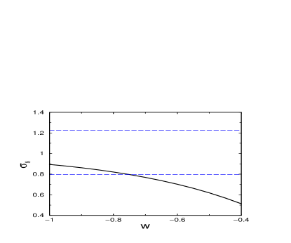
To be more specific, the suppression of growth affects the overall normalization of the power spectrum today, most easily expressed in terms of the rms mass fluctuations in spheres of $8h^{-1}\,$Mpc, or $\sigma_{8}$ (see Fig. 3). Further, the number density of bound objects formed by a given redshift is exponentially sensitive to the growth of density perturbations bahcall . The number density can be accurately estimated by the Press-Schechter formalism PS ,

$$\hskip 28.45274pt\frac{dn}{dM}(z,M)=$$

$$\sqrt{\frac{2}{\pi}}\frac{\rho_{M}}{M}\frac{\delta_{c}}{\sigma(M,z)^{2}}\frac{d\sigma(M,z)}{dM}\exp\left(-\frac{\delta_{c}^{2}}{2\sigma(M,z)^{2}}\right)$$ (4)

where $\sigma(M,z)$ is the rms density fluctuation on mass-scale $M$ evaluated at redshift $z$ and computed using linear theory, $\rho_{M}$ is the present-day matter density, and $\delta_{c}\approx 1.68$ is the linear threshold overdensity for collapse.

Strong and weak gravitational lensing may be used to constrain the growth of structure and thus probe the dark energy. We will not address them here as detailed modeling of the lenses, their distribution, and the evolution of non-linear structure is required to address their efficacy. We refer the reader to Refs. lensing . The effect of dark energy on the growth of linear density perturbations enters in the cluster-number-count test, as discussed below.

Figure 3: The rms amplitude of matter perturbations on the scale $8h^{-1}\,$Mpc as a function of (constant) $w$ for a COBE normalized, scale-invariant model with $h=0.7$ (see Ref. turner_white for details). The present cluster abundance fixes $\sigma_{8}=(0.56\pm 0.1)\Omega_{M}^{-0.47}$ (95% cl) viana_liddle , indicated by the broken lines for $\Omega_{M}=0.3$. The downward trend in $\sigma_{8}$ with increasing $w$ is the suppression of the growth of linear density perturbations as dark energy domination occurs earlier, and leads to an upper limit to $w$ of around $-1/2$.

II.2 Classical tests

The other cosmological probes of the dark energy involve the classical tests: magnitude vs. redshift (Hubble) diagram, number-count vs. redshift, and angular size vs. redshift. For the flat models that we consider, all of these depend upon the comoving distance to an object at redshift $z$, which is determined by the expansion history:

$$r(z)=\int_{0}^{z}\,{dx\over H(x)}\,.$$ (5)

Luminosity distance, which is the distance inferred from measurements of the apparent luminosity of an object of known intrinsic luminosity, $\log(d_{L}(z))\equiv 0.2(m-M)-5$, is related to $r(z)$

$$d_{L}(z)=(1+z)r(z),$$ (6)

where $m$ is apparent luminosity, $M$ the absolute luminosity and distances are measured in Mpc. The magnitude – redshift (Hubble) diagram is a plot of $m(z)$ vs. $z$.

The angular-diameter distance, which is the distance inferred from the angular size of an object of known size, $d_{A}(z)=D/\theta$, is related to $r(z)$

$$d_{A}=r(z)/(1+z).$$ (7)

The angular-diameter distance comes into play in using CMB anisotropy (more below) or the Alcock-Paczynski test to probe the dark energy.

The Alcock-Paczynski compares the angular size of an object on the sky with its the redshift extent APtest . The diameter $D$ of a spherical object (of fixed size or comoving with the expansion) at redshift $z$ is related to its angular size on the sky $d\theta$ by $d_{A}(z)d\theta$ and to its redshift extent by $\Delta z/(1+z)H(z)$. Thus, measurements of $\Delta z$ and $\Delta\theta$ can be combined to determine $H(z)r(z)$:

$$H(z)r(z)={\Delta z\over\Delta\theta}$$ (8)

The trick is to find objects (or ensembles of objects) that are spherical. One idea involves the correlation function of galaxies or of Lyman-$\alpha$ clouds, which, because of the isotropy of the Universe, should have the same dependence upon separation along the line-of-sight or across the sky. A large and uniform sample of objects is needed to implement this test; further, the effects of peculiar velocities induced by density perturbations must be separated from the small (5% or so) cosmological effect ballinger .

The authors of Ref. lamhuietal have discussed the feasibility of using the correlation function of Lyman-$\alpha$ clouds seen along the lines-of-sight of neighboring high-redshift quasars to distinguish between a low-density model and a flat model with dark energy. Fig. 4 shows the sensitivity of this technique to $w$; whether or not it has the power to probe the nature of the dark energy remains to be seen.

The comoving volume element is the basis of number-count tests (e.g., counts of lensed quasars, galaxies, or clusters of galaxies). It is given in terms of $r(z)$ and $H(z)$

$$f(z)\equiv{dV\over dzd\Omega}=r^{2}(z)/H(z)\,.$$ (9)

Note too that

$$f(z)={dF(z)\over dz}\qquad F(z)=\int_{0}^{z}\,f(z)dz={r(z)^{3}\over 3}\,.$$ (10)

Figure 4: The Alcock-Paczynski test, which compares the angular size ($\Delta\theta$) of a spherical object at redshift $z$ to its redshift extent ($\Delta z$), can determine $r(z)H(z)$. Its sensitivity is shown here for $\Omega_{M}=0.3$ and constant $w=-0.4,-0.6,-0.8,-1.0$.

Figure 5: Comoving volume element $f(z)=dV/d\Omega dz$ vs. redshift for constant $w=-1,-0.8,-0.6,-0.4$ (from top to bottom).

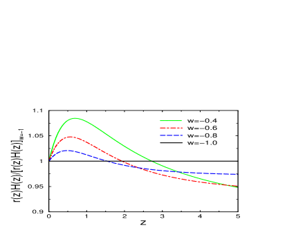
The ability of these cosmological observables to probe the dark-energy equation-of-state depends upon their sensitivity to $w$. To begin, consider the case of constant $w$. The sensitivity of $r(z)$, $H(z)$ and $f(z)$ to $w$ is quantified by

$${dr(z)\over dw} = -{3\over 2}\int_{0}^{z}\,{\Omega_{X}H_{0}^{2}(1+x)^{3(1+w)}\ln(1+x)\,dx\over H^{3}(x)}$$ (11)

$${df(z)\over dw} = {2r(z)\over H(z)}{dr\over dw}-{r(z)^{2}\over H(z)^{2}}{dH\over dw}$$ (12)

$${dH(z)\over dw} = {3\over 2}{\Omega_{X}H_{0}^{2}(1+z)^{3(1+w)}\ln(1+z)\over H(z)}$$ (13)

The comoving distance to an object at redshift $z$ and its sensitivity to $w$ is shown in Fig. 6. At small redshifts $r(z)$ is insensitive to $w$ for the simple reason that all cosmological models reduce to the Hubble law ($r=H_{0}^{-1}z$) for $z\ll 1$,

$$r(z)\rightarrow H_{0}^{-1}\left[z-{3\over 4}z^{2}-{3\over 4}\Omega_{X}wz^{2}+\cdots\right]\ \ {\rm for}\ z\ll 1$$ (14)

At redshift greater than about five, the sensitivity of $r(z)$ to a change in $w$ levels off because dark energy becomes an increasingly smaller fraction of the total energy density, $\rho_{X}/\rho_{M}\propto(1+z)^{3w}$. As we shall discuss later, the fact that $dr/dw$ increases monotonically with redshift means that for measurements of fixed error, one would want to make the measurement at the highest redshift possible in order to minimize the uncertainty in the inferred value of $w$.

Figure 6: $r(z)$ and $dr/dw$ as a function of $z$ (in units of $H_{0}^{-1}$) for $\Omega_{M}=0.3$ and $w=-1$.

Figure 7: The relative sensitivity of $r(z)$, $f(z)$, and $H(z)$ to a change in the constant value of $w$.

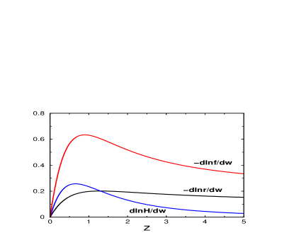
Fig. 7 shows the relative change in $r(z)$ and in the comoving volume element $f(z)$ due to a change in $w$ as a function of redshift. The sensitivities of $r(z)$ and $f(z)$ peak at redshifts around unity. The reason for decreased sensitivity at small and large redshifts is as discussed just above.

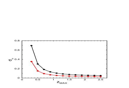
As noted earlier, observations at redshifts $0\mathrel{\mathchoice{\lower 3.6pt\vbox{\halign{$\mathsurround=0pt\displaystyle\hfil#\hfil$\cr<\crcr\sim\crcr}}}{\lower 3.6pt\vbox{\halign{$\mathsurround=0pt\textstyle\hfil#\hfil$\cr<\crcr\sim\crcr}}}{\lower 3.6pt\vbox{\halign{$\mathsurround=0pt\scriptstyle\hfil#\hfil$\cr<\crcr\sim\crcr}}}{\lower 3.6pt\vbox{\halign{$\mathsurround=0pt\scriptscriptstyle\hfil#\hfil$\cr<\crcr\sim\crcr}}}}z\mathrel{\mathchoice{\lower 3.6pt\vbox{\halign{$\mathsurround=0pt\displaystyle\hfil#\hfil$\cr<\crcr\sim\crcr}}}{\lower 3.6pt\vbox{\halign{$\mathsurround=0pt\textstyle\hfil#\hfil$\cr<\crcr\sim\crcr}}}{\lower 3.6pt\vbox{\halign{$\mathsurround=0pt\scriptstyle\hfil#\hfil$\cr<\crcr\sim\crcr}}}{\lower 3.6pt\vbox{\halign{$\mathsurround=0pt\scriptscriptstyle\hfil#\hfil$\cr<\crcr\sim\crcr}}}}2$ will be most useful in probing the dark energy. This fact is made more quantitative in Fig. 8, which shows the accuracy of the determination of the equation-of-state $w$ (assumed constant) using 2000 SNe Ia, as a function of maximum redshift probed $z_{\rm max}$. For $0.2\mathrel{\mathchoice{\lower 3.6pt\vbox{\halign{$\mathsurround=0pt\displaystyle\hfil#\hfil$\cr<\crcr\sim\crcr}}}{\lower 3.6pt\vbox{\halign{$\mathsurround=0pt\textstyle\hfil#\hfil$\cr<\crcr\sim\crcr}}}{\lower 3.6pt\vbox{\halign{$\mathsurround=0pt\scriptstyle\hfil#\hfil$\cr<\crcr\sim\crcr}}}{\lower 3.6pt\vbox{\halign{$\mathsurround=0pt\scriptscriptstyle\hfil#\hfil$\cr<\crcr\sim\crcr}}}}z_{\rm max}\mathrel{\mathchoice{\lower 3.6pt\vbox{\halign{$\mathsurround=0pt\displaystyle\hfil#\hfil$\cr<\crcr\sim\crcr}}}{\lower 3.6pt\vbox{\halign{$\mathsurround=0pt\textstyle\hfil#\hfil$\cr<\crcr\sim\crcr}}}{\lower 3.6pt\vbox{\halign{$\mathsurround=0pt\scriptstyle\hfil#\hfil$\cr<\crcr\sim\crcr}}}{\lower 3.6pt\vbox{\halign{$\mathsurround=0pt\scriptscriptstyle\hfil#\hfil$\cr<\crcr\sim\crcr}}}}1$, the $1\sigma$ uncertainty $\sigma_{w}$ decreases sharply and then levels, with little decrease for $z_{\rm max}\mathrel{\mathchoice{\lower 3.6pt\vbox{\halign{$\mathsurround=0pt\displaystyle\hfil#\hfil$\cr>\crcr\sim\crcr}}}{\lower 3.6pt\vbox{\halign{$\mathsurround=0pt\textstyle\hfil#\hfil$\cr>\crcr\sim\crcr}}}{\lower 3.6pt\vbox{\halign{$\mathsurround=0pt\scriptstyle\hfil#\hfil$\cr>\crcr\sim\crcr}}}{\lower 3.6pt\vbox{\halign{$\mathsurround=0pt\scriptscriptstyle\hfil#\hfil$\cr>\crcr\sim\crcr}}}}1.5$.

Figure 8: $1\sigma$ accuracy in the determination of constant $w$ as a function of maximum redshift probed $z_{\rm max}$ for a flat Universe, 2000 SNe and marginalizing over the other parameter, $\Omega_{M}$. The upper curve shows the uncertainties using the fiducial SNAP dataset, while the lower curve shows uncertainties obtained the mathematically optimal strategy (see Sec. V). For all $z_{\rm max}$, 2000 SNe were used, with a redshift distribution as shown in Fig. 12 for the upper curve.

II.3 CMB anisotropy

Figure 9: COBE-normalized angular power spectrum of CMB anisotropy for a flat model with $\Omega_{B}h^{2}=0.02$, $\Omega_{X}=0.7$, $h=0.65$ and $w=-1$, obtained using CMBFAST CMBFAST . The acoustic peaks correspond to modes that at the moment of last scattering are at maximum compression (odd) or rarefaction (even).

The gravity-driven acoustic oscillations of the baryon-photon fluid at the time of last scattering gives rises to a series of acoustic peaks in the angular power spectrum of CMB anisotropy (see Fig. 9) hu_sugiyama . The CMB is a snapshot of the Universe at $z=z_{\rm LS}\simeq 1100$ and the peaks correspond to different Fourier modes caught at maximum compression or rarefaction, when the fluctuation in the photon temperature is at an extremum. The condition for this is $k\eta_{\rm SH}\simeq n\pi$, where the odd (even) $n$ modes are compression (rarefaction) maxima and $\eta_{\rm SH}$ is the sound horizon:

$$\eta_{\rm SH} = \int_{0}^{t_{\rm LS}}\,{v_{s}\,dt\over R(t)}=\int_{z_{\rm LS}}^{\infty}{v_{s}(z^{\prime})dz^{\prime}\over H(z^{\prime})}$$ (15)

$$v_{s}^{2} = 1/3\over 1+{3\rho_{B}/4\rho_{\gamma}}$$ (16)

Modes captured at maximum compression or rarefaction provide standard rulers on the last-scattering surface with physical sizes $d\sim\pi/k\,(1+z_{\rm LS})\sim\eta_{\rm SH}/n\,(1+z_{\rm LS})$ Their angular sizes on the CMB sky are given by

$$\theta_{n} \sim {\eta_{\rm SH}/n\over(1+z_{\rm LS})d_{A}(z_{\rm LS})}$$ (17)

$$d_{A}({\rm LS}) = (1+z_{\rm LS})^{-1}\int_{0}^{z_{\rm LS}}{dz^{\prime}\over H(z^{\prime})}$$ (18)

This can be made more precise for the angular power spectrum. The angular power at multipole $l$ is dominated by modes around $k\simeq l/\eta_{\rm LS}$, and so the positions of the peaks are given approximately by (see, e.g., Ref. weinberg_peaks )

$$l_{n}=n\pi{\eta_{\rm LS}\over\eta_{\rm SH}}\,.$$ (19)

For a flat Universe $\eta_{\rm LS}$ is just the coordinate distance to the last-scattering surface $r(z_{\rm LS})$.

The positions of the acoustic peaks are the primary sensitivity the CMB has to the equation-of-state of the dark energy (see Fig. 10). Most of that sensitivity arises from the dependence of the distance to the last-scattering surface upon the time history of $w$. Using the approximation above, and taking into account the other important cosmological parameters, it follows that

$${\Delta l_{1}\over l_{1}} = -0.084\Delta w-0.23{\Delta\Omega_{M}h^{2}\over\Omega_{M}h^{2}}+0.09{\Delta\Omega_{B}h^{2}\over\Omega_{B}h^{2}}$$ (20)

$$\hskip 19.91684pt+0.089{\Delta\Omega_{M}\over\Omega_{M}}-1.25{\Delta\Omega_{0}\over\Omega_{0}}$$

around $w=-1$, $h=0.65$, $\Omega_{M}=0.3$, $\Omega_{B}h^{2}=0.02$ and $\Omega_{0}=1$. Other features of the CMB power spectrum (e.g., heights of the acoustic peaks and damping tail) can precisely determine the matter density ($\Omega_{M}h^{2}$) and the baryon density ($\Omega_{B}h^{2}$); therefore, for a flat Universe the main dependence of the position of the acoustic peaks is upon $\Omega_{M}$ and $w$. For $\Omega_{M}\sim 0.3$, $l_{1}$ is about three times more sensitive to $\Omega_{M}$ than $w$. Interestingly enough, the recent data from the BOOMERanG and MAXIMA-1 experiments indicate that the first peak is located at around $l\simeq 200$ Jaffe , which indicates a larger value of $w$, $w\sim-0.6$, than the supernova data and suggests the dark energy may be something other than a cosmological constant. However, there is little statistical significance to this result.

(The CMB angular power spectrum has additional sensitivity to dark energy which is not captured by Eq. (20). It arises through the late-time ISW effect and the slight clumping of dark energy, and mainly affects the low-order multipoles. Because of the large cosmic variance at large scales, this dependence is not likely to significantly enhance the ability of CMB anisotropy to probe $w$.)

Figure 10: The position of the first acoustic peak as a function of $w$ for $\Omega_{B}h^{2}=0.02$ and $\Omega_{M}h^{2}=0.13$.

II.4 Time-varying $w$

There is no compelling reason to believe that the dark energy is characterized by a constant $w$. In particular, if the dark energy is associated with an evolving scalar field then the effective equation-of-state,

$$w(t)\equiv p_{\phi}/\rho_{\phi}={{1\over 2}\dot{\phi}^{2}-V(\phi)\over{1\over 2}\dot{\phi}^{2}+V(\phi)},$$ (21)

is in general time-varying. Thus, sensitivity to the value of $w(z)$ at a given $z$ is an important measure of the probative power of a given test. Needless to say, in order to probe the variation of $w$ with redshift, one has to perform measurements at different redshifts. Thus, CMB anisotropy and the age of the Universe cannot probe this aspect of the dark energy; rather, they can only measure some average value of $w$.

We now consider the effect of a change in $w$ at redshift $z_{*}$; specifically, a change in $w$ over a small redshift interval around $z=z_{*}$, such that $\int\delta w(z)d\ln z=1$. The effect on $H(z)$ for $z>z_{*}$, which we denote by the functional derivative $\delta H/\delta w(z)$, is

$${\delta H(z)\over\delta w(z)}={3\over 2}{z_{*}\over 1+z_{*}}{\Omega_{X}H_{0}^{2}\exp\left[3\int_{0}^{z}(1+w)d\ln(1+z)\right]\over H(z)}$$ (22)

and zero for $z<z_{*}$. Note that the effect of $\delta w(z)$ on the expansion rate is essentially to change it by a fixed amount for $z>z_{*}$.

The effect on $r(z)$ and $f(z)=r(z)^{2}/H(z)$ follows by simple calculus:

$${\delta\ln r\over\delta w(z)} = {1\over r(z)}\int_{0}^{z}\left(-{\delta H\over\delta w}\right){dz\over H(z)^{2}}$$ (23)

$${\delta\ln f\over\delta w} = {2}{\delta\ln r\over\delta w}-{1\over H(z)}{\delta H\over\delta w}$$ (24)

The sensitivity of $r(z)$ and $f(z)$ to a localized change in $w$ is shown in Fig. 11, where we take $z_{*}=0.9z$. Both $r(z)$ and the comoving volume element are insensitive to the value of $w(z)$ at small redshift (since $r$ and $H$ are insensitive to the form of the dark energy) and at large redshifts (because $\rho_{X}/\rho_{M}$ decreases rapidly). They are most sensitive to $w(z)$ over the redshift range $z\sim 0.2-1.5$, with the sweet spot being at $z\approx 0.4$.

Figure 11: The relative sensitivity of the comoving distance $r(z)$ and the comoving volume element $f(z)$ to a localized change in the value of $w$ at redshift $z_{*}$ characterized by $\int\delta w(z)d\ln z=1$.

As discussed in Ref. hutererturner , measurements of $r(z)$ can in principle be used to reconstruct the equation-of-state (or scalar-field potential in the case of quintessence). The reconstruction equation for $w(z)$ is

$$1+w(z)={1+z\over 3}\,{3H_{0}^{2}\Omega_{M}(1+z)^{2}+2(d^{2}r/dz^{2})/(dr/dz)^{3}\over H_{0}^{2}\Omega_{M}(1+z)^{3}-(dr/dz)^{-2}}.$$ (25)

This equation can be used to illustrate yet again the difficulty of probing the dark energy at high redshift. Suppose that $r(z)$ and its derivatives are measured very accurately and that the only uncertainty in reconstructing $w(z)$ is due to $\Omega_{M}$. The uncertainty in $w(z)$ due to the uncertainty in $\Omega_{M}$ can be obtained by differentiating Eq. (25) with respect to $\Omega_{M}$:

$$\Delta w(z) = {-(1+z)^{3}\over\Omega_{X}\exp\left[3\int(1+w)\,d\ln(1+z)\right]}\,\Delta\Omega_{M}$$ (26)

$$\rightarrow {-(1+z)^{-3w}\over\Omega_{X}}\,\Delta\Omega_{M}\ \ \ ({\rm const\ }w)$$ (27)

Therefore, the uncertainty in $w(z)$ increases with redshift sharply, as $(1+z)^{-3w}$. This happens because $w<0$ and the dark energy constitutes an increasingly smaller fraction of the total energy at high redshift.

The reconstruction equations based upon number counts can simply be obtained by substituting $[3F(z)]^{1/3}$ for $r(z)$ in Eq. (25). Since the expansion history $H(z)$ can in principle be obtained from measurements of $f(z)$ and $r(z)$ (number counts and Hubble diagram), or from $r(z)$ and $r(z)H(z)$ (Hubble diagram and Alcock-Paczynski test), with a sense of great optimism we write the reconstruction equation based upon a determination of $H(z)$:

$$1+w(z)={1\over 3}{2(1+z)H^{\prime}(z)H(z)-3H_{0}^{2}(1+z)^{3}\Omega_{M}\over H^{2}(z)-H_{0}^{2}\Omega_{M}(1+z)^{3}}$$ (28)

which follows from

$$dr(z) = -dt/a(t)=dz/H(z).$$ (29)

This reconstruction equation has the virtue of depending only upon the first derivative of the empirically determined quantity.

II.5 Summing up

In sum, the properties of the dark energy are best revealed by probes of the low-redshift ($z\sim 0.2-2$) Universe – SNe Ia, number-counts and possibly the Alcock-Paczynski test. The CMB has an important but more limited role to play since it can only probe an average value of $w$. SNe Ia are currently the most mature probe of the dark energy, and already impose significant constraints on $w$ garnavich ; perl_tur_white ; perlmutter-1999 , $w<-0.6$ (95% CL). The efficacy of any of these tests will depend critically upon the identification and control of systematic error (more late).

The classical cosmological tests that involve $r(z)$ alone have the virtue of only depending upon $\Omega_{M}$, $\Omega_{X}$ and $w$, which can be reduced to two parameters ($\Omega_{M}$ and $w$) with a precision measurement of $\Omega_{0}$ from the CMB. CMB anisotropy on the other hand depends upon a large number of parameters (e.g., $\Omega_{B}h^{2}$, $h$, $n$, $dn/d\ln k$, ionization history, etc). The number-count tests can also depend upon the growth of structure which brings in other parameters that affect the shape of the power spectrum (e.g. $n$, $\Omega_{B}h^{2}$, $h$).

In the remainder of this paper we pay special attention to SNe Ia, and in particular consider how well the dark energy could be probed by a high-quality dataset provided by the proposed satellite mission SNAP SNAP . As the fiducial dataset, we consider a total of 2000 SNe Ia with individual statistical uncertainties of $0.15$ mag (the impact of systematic uncertainties to this dataset was studied in Refs. SNAP ; weller ; astier ). The bulk of the SNe are assumed to have $0.2<z<1.2$, with about a hundred at $1.2<z<1.7$ and another two hundred or so at $z<0.2$. The low-z sample is expected from near-future ground searches, such as the Nearby Supernova Factory SN_factory .

Figure 12: Histogram of projected SNe Ia distribution from SNAP. The number of SNe at $z>1.2$ is smaller because spectra of SNe at such high $z$ are redshifted into the infrared region, where observations are more difficult. About 200 SNe at $z<0.2$ are assumed to be provided by ground-based SNe searches.

The number-count technique can be implemented in a variety of ways — for example, halos of a fixed mass davis , clusters of galaxies of fixed mass holder , and gravitationally lensed quasars coorayhuterer . All of these methods, however, are susceptible to redshift evolution of the objects in question, as well as considerable uncertainties in theoretical modeling.

Unless otherwise indicated, we use the Fisher-matrix formalism throughout to estimate uncertainties Fisher-Jungman ; Fisher-Tegmark . In several instances we have checked that the values obtained agree well with those using Monte-Carlo simulation. The fiducial cosmological model is $\Omega_{M}=1-\Omega_{X}=0.3$, $w=-1$, unless otherwise indicated.

III Constraints on (constant) $w$

To begin, we assume that the equation-of-state of the dark energy does not change in time, $w(z)=w={\rm const}$. Not only does this hold for models with truly constant $w$ (vacuum energy, domain walls and cosmic strings, etc.) but models with time-variable equation-of-state can have $w\approx{\rm const}$ out to $z\sim 2$.

III.1 SNe Ia and CMB

Figure 13: Projected SNAP constraint compared to those projected for MAP and Planck (with polarization information) and SDSS (MAP, Planck and SDSS constraints are from Ref. hu_obs_99 ). Also shown are the present constraints using a total of 54 SNe Ia. All constraints assume a flat Universe and $\Omega_{M}=1-\Omega_{X}=0.28$, $w=-1$ as fiducial values of the parameters. All contours are 68% cl, and were obtained using the Fisher-matrix analysis.

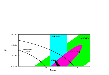
Fig. 13 shows that a supernova program, such as SNAP SNAP , will enable very accurate measurement of $w$: $\sigma_{w}\approx 0.05$, after marginalization over $\Omega_{M}$ and assuming a flat Universe. This figure also shows constraints anticipated from the Sloan Digital Sky Survey (SDSS) and MAP and Planck satellites (with polarization information). As expected, the fact that the dark energy is smooth on observable scales implies that its properties cannot be probed well by galaxy surveys.

The CMB, on the other hand, is weakly sensitive to the dark energy, mainly through the dependence of the distance to the surface of last scattering upon $w$. The orientation of the CMB ellipses is roughly predicted from Eq. (20), indicating that this equation captures most of the CMB dependence upon dark energy.

The CMB provides only a single measurement of the angular-diameter distance to the surface of last scattering, albeit an accurate one. In the case of Planck, the angular-diameter distance to the last-scattering surface is measured to 0.7% eisen-private . Fig. 13 illustrates that ultimately CMB is not likely to be as precise as a well-calibrated SNe dataset. It does provide complementary information and a consistency check. However, combining SNAP and Planck improves the SNAP constraint only by about 5-10%.

The uncertainty in the determination of $w$ varies as a function of the central value of this parameter. As $w$ increases from $-1$, the SNe constraint becomes weaker: the variation of dark energy with redshift becomes similar to that of matter, and it is more difficult to disentangle the two components by measuring the luminosity distance. For example, for $w=-0.7$ and keeping $\Omega_{M}=0.3$, the constraints on these two parameters from SNAP deteriorate by 10% and 50% respectively relative to the $w=-1$ case. On the other hand, the CMB constraint becomes somewhat stronger with increasing $w$ because the ISW effect increases (see Fig. 5 in Ref. hu_obs_99 ).

III.2 Number-counts

Figure 14: Constraints in the $\Omega_{M}$-$w$ plane using galaxy-halo counts from the DEEP survey davis . Inner most region shows the constraint assuming Poisson errors only, while the outer two regions assume an additional, irreducible uncertainty of 10% and 20% (per bin) in the comoving number density of halos due to evolution. All regions are 68% cl.

Davis and Newman davis have argued that the comoving abundance of halos of a fixed rotational speed (nearly fixed mass) varies weakly with the cosmological model and can be calibrated with numerical simulations, leaving mostly the dependence on the volume element davis . We follow these authors in assuming 10000 galaxy halos divided into 8 redshift bins at $0.7<z<1.5$. The redshift range for the DEEP survey roughly corresponds to the redshift range of greatest sensitivity to dark energy.

Fig. 14 shows the constraints obtained using the Fisher-matrix formalism assuming Poisson errors only, and then allowing for an additional 10% or 20% error per bin for the uncertainty in the evolution of the comoving halo density. Assuming no uncertainty in the comoving halo density, the error ellipse is similar to that of SNAP. However, allowing for a modest uncertainty due to evolution (10 or 20%), the size of the error ellipse increases significantly. Finally, we note that any probe sensitive primarily to $dV/d\Omega dz$ will have its error ellipse oriented in the direction shown.

Figure 15: Projected one, two and three $\sigma$ constraints on $\Omega_{M}$ and $w$ in a flat Universe using counts of galaxy clusters (adopted from Ref. holder ) for an x-ray selected sample of thousand clusters (top panel) and a Sunyaev-Zel’dovich selected sample of hundred clusters (bottom).

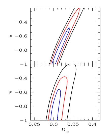
While clusters are simpler objects than galaxies, they are “rare objects” and their abundance depends exponentially upon the growth of density perturbations and varies many orders-of-magnitude over the redshift range of interest bahcall . The sensitivity to the growth factor outweighs that of the cosmological volume, and the error ellipses for the cluster number-count test are almost orthogonal to the halo-number count test (see Fig. 15). The information provided is thus complementary to halo counts and SNe data.

Because of the exponential dependence of the abundance, control of the systematic and modeling errors is critical. Especially important is accurate determination of cluster masses (use of weak-gravitational lensing to determine cluster masses might be very useful gilholder ). Shown in Fig. 15 are the estimated constraints for sample of a hundred clusters with $0<z<3$ selected in a future Sunyaev-Zel’dovich survey and a thousand clusters with $0<z<1$ selected in a future x-ray survey holder . These cluster constraints are comparable and complementary to those of the halo counts when a 20% uncertainty in halo-number evolution is taken into account.

IV Probing the Time-history of Dark Energy

Although some of the models for the dark energy, such as the vacuum energy, cosmic defects and some quintessence models produce $w={\rm const}$ (at least out to redshifts of a few), the time-variation of $w$ is a potentially important probe of the nature of dark energy. For example, evolving scalar field models generically time-variable $w$. Moreover, in some cases (e.g. with PNGB scalar field models coble and some tracker quintessence models zlatev ) $w(z)$ can exhibit significant variation out to $z\sim 1$.

IV.1 Constraining the redshift dependence of $w$

Given a dark-energy model it is easy to compute $w(t)$ and from it the prediction for $r(z)$. There is little theoretical guidance as to the nature of the dark energy, so we seek ways to parameterize $w(z)$ as generally as possible. A further complication is the degeneracy of $w(z)$ with $\Omega_{M}$ and $\Omega_{X}$. To make useful progress, we assume that by the time a serious attempt is made to probe the rate of change of $w$, $\Omega_{M}$ and $\Omega_{X}$ will be measured accurately (e.g., $\Omega_{M}+\Omega_{X}$ from CMB anisotropy, and $\Omega_{M}$ from large-scale structure surveys).

IV.2 Case I: $w(z)=w_{1}+w^{\prime}(z-z_{1})$

Figure 16: Here $w(z)$ was Taylor-expanded around $z_{1}=0.31$ with fiducial model $w(z)=-0.8+0.1\,z$. The top panel shows 68% and 95% cl constraints in the $w_{1}$-$w^{\prime}$ plane. The bottom panel shows the same constraint in the $w$-$z$ plane, with the fiducial model (heavy line) and confidence regions (shaded). The broken lines in both panels should the effect of assuming a Gaussian uncertainty of $0.05$ in $\Omega_{M}$.

The simplest way to parameterize the rate of change of $w$ is to write the first-order Taylor expansion

$$w(z)=w_{1}+w^{\prime}(z-z_{1}),$$ (30)

where $w_{1}=w(z=z_{1})$ and $w^{\prime}\equiv(dw/dz)_{z=z_{1}}$ are constants and $z_{1}$ is the redshift around which we expand (chosen according to convenience or theoretical prejudice). The energy density in the dark component is then given by

$$\rho_{X}(z)=\rho_{X}(0)(1+z)^{3(1+w_{1}-w^{\prime}(1+z_{1}))}\exp(3w^{\prime}\,z).$$ (31)

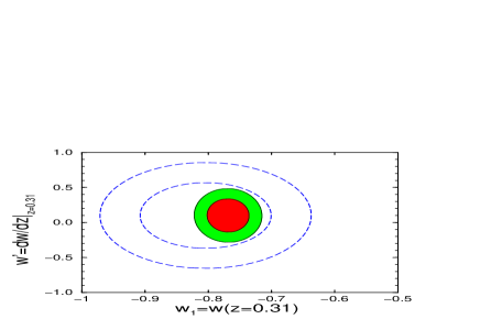
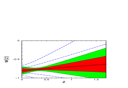
Using the Fisher-matrix formalism, we determine the error ellipses in the $w_{1}$-$w^{\prime}$ plane. We choose $z_{1}$ so that $w_{1}$ and $w^{\prime}$ become uncorrelated, (how to do this analytically is shown in Ref. Eisenstein ). For uncorrelated $w_{1}$ and $w^{\prime}$, the constraint to $w(z)$ follows by computing

$$\sigma_{w(z)}=\left[\sigma_{w_{1}}^{2}+\sigma_{w^{\prime}}^{2}\,(z-z_{1})^{2}\right]^{1/2}.$$ (32)

Fig. 16 illustrates the error ellipse for $w_{1}$ and $w^{\prime}$ (top panel) and the constraint to $w(z)$ (bottom panel). As we discussed in Sec. II, cosmological observations have diminishing leverage at both high and low redshift, which is reflected in the narrow “waist” at $z\sim 0.35$, and this is the sweet spot in sensitivity to $w(z)$ (see Fig. 11).

The uncertainty in the slope, $\sigma_{w^{\prime}}=0.16$, is about 8 times as large as that in $w(z_{1})$, $\sigma_{w_{1}}=0.02$. Despite the relatively large uncertainty in $w^{\prime}$, this analysis may be useful in constraining the dark-energy models.

Finally, we also show in Fig. 16 the significant effect of a Gaussian uncertainty of $0.05$ in $\Omega_{M}$; it roughly doubles $\sigma_{w_{1}}$ and $\sigma_{w^{\prime}}$ and moves the value of $z_{1}$ that decorrelates the two parameters to less than zero.

IV.3 Case II: $w(z)=w_{1}-\alpha\ln[(1+z)/(1+z_{1})]$

There are other ways to parameterize the variation of $w(z)$ with redshift. Efstathiou efstathiou argues that many quintessence models produce equation-of-state ratio that is well approximated by $w(z)=w_{0}-\alpha\ln(1+z)$ with $w_{0}$ and $\alpha$ constants. We generalize this by expanding around an arbitrary redshift $z_{1}$

$$w(z)=w_{1}-\alpha\ln\left({1+z\over 1+z_{1}}\right).$$ (33)

Here, the energy density in the dark energy evolves as

$$\rho_{X}(z) = \rho_{X}(0)(1+z)^{3(1+w_{1}+\alpha\ln(1+z_{1}))}\times$$ (35)

$$\exp\left[-{3\over 2}\,\alpha\ln^{2}(1+z)\right].$$

As with the Taylor expansion, we have a 2-parameter form for $w(z)$ and, using the supernova data, we examine the constraints that can be imposed on $w_{1}$ and $\alpha$. We again choose $z_{1}$ so that $w_{1}$ and $\alpha$ are decorrelated; this occurs for $z_{1}=0.30$.

Figure 17: Here the dark energy is parameterized by $w(z)=w_{1}-\alpha\ln[(1+z)/(1+z_{1})]$, with $w_{1}=-0.75$ and $\alpha=-0.2$. The top panel shows 68% and 95% cl constraints in the $w_{1}$-$\alpha$ plane. The bottom panel shows the same constraint in the $w$-$z$ plane, with the fiducial model (heavy line) and 68% and 95% cl confidence region (shaded).

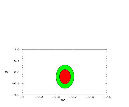
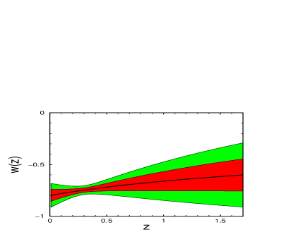
Fig. 17 shows 68% and 95% cl constraint regions in the $w_{1}$-$\alpha$ plane (top panel) and $w$-$z$ plane (bottom). The fiducial model ($w_{1}=-0.75$, $\alpha=-0.2$) is chosen to produce $w(z)$ similar to that from linear expansion (Case I). The uncertainty in parameter determination is $\sigma_{w_{1}}=0.02$ and $\sigma_{\alpha}=0.21$. The bottom panel of this figure shows that using the logarithmic expansion we obtain similar constraints to $w(z)$ as with the linear expansion. This is not surprising, as near the leverage point $z_{1}\approx 0.3$, the two expansions are essentially equivalent with $\alpha=(1+z_{1})w^{\prime}$ and $\sigma_{\alpha}=(1+z_{1})\sigma_{w^{\prime}}$, which is consistent with our results.

IV.4 Case III: Constant $w$ in redshift bins

An even more general way to constrain $w(z)$ is to parameterize it by constant values in several redshift bins, since no particular form for $w(z)$ need be assumed. Of course, more redshift bins lead to weaker constraints in each bin.

We divide the SNAP redshift range into $B$ bins centered at redshifts $z_{i}$ with corresponding widths $\Delta z_{i}$ and equation-of-state ratios $w_{i}$ ($i=1,\ldots,B$). The energy density of the dark component evolves as ($z_{j-1}<z<z_{j}$)

$$\rho_{X}(z) = \rho_{X}(z=0)\,\prod_{i=1}^{j-1}\left(\frac{1+z_{i}+\Delta z_{i}/2}{1+z_{i}-\Delta z_{i}/2}\right)^{3(1+w_{i})}\times$$ (36)

$$\left(\frac{z}{1+z_{j}-\Delta z_{j}/2}\right)^{3(1+w_{j})}.$$

To obtain the constraints using this approach, we again employ the Fisher matrix formalism, treating $w_{i}$ as the parameters to be determined.

Figure 18: Here $w(z)$ is parameterized by constant values in redshift bins. The outer region shows 68% cl constraints corresponding to each redshift bin. The inner region shows 68% cl constraints when, in addition, a Gaussian prior is imposed that penalizes models with a large change in $w$ between two adjacent bins.

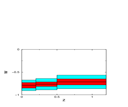
Fig. 18 shows constraints on $w(z)$ when $w$ is parameterized by values in three redshift bins whose widths are chosen so that the uncertainty in each is about the same. Precise knowledge of $\Omega_{M}$ and $\Omega_{X}$ was assumed.

The constraints are not strong ($\sigma_{w}\approx 0.12$) in part because the values of $w$ in adjacent bins are uncorrelated. Most realistic models with time-dependent equation-of-state have $w(z)$ that varies slowly (or doesn’t vary at all) out to $z\sim 1$. Therefore, we also show results when a Gaussian prior is imposed that penalizes models with large change in $w$ between two adjacent bins ($\sigma_{w}=0.10$ for change in $\Delta w_{i}$ between adjacent bins). The $1\sigma$ constraints improve by more than a factor of two.

IV.5 Non-parametric Reconstruction

The most general approach is the direct reconstruction of $w(z)$ from the measured luminosity distance – redshift relation provided by the SNe Ia data hutererturner ; chiba ; saini ; chiba2 . This method is non-parametric and no assumptions about the dark energy or its equation-of-state are needed. This is also the most challenging approach, since the reconstructed potential and equation-of-state ratio will depend on first and second derivatives of the distance with respect to redshift, cf. Eq. (25). This leads to a fundamental problem: even very accurate and dense measurements of $r(z)$ allow great freedom in $r^{\prime}\equiv dr/dw$ and $r^{\prime\prime}\equiv d^{2}r/dw^{2}$, because they themselves are not probed directly.

To address this problem, various authors have advocated polynomials and Padé approximants hutererturner and various fitting functions saini ; chiba2 ; weller to represent $r(z)$ and thereby reduce the inherent freedom in $r^{\prime}$ and $r^{\prime\prime}$.

Figure 19: Reconstruction of the quintessence model with potential $V(\phi)=M^{4}[\exp({m_{\rm Pl}}/{\phi})-1]$ zlatev and $\Omega_{X}=0.50$. The solid line is the input model, and the shaded regions are the 68% and 95% confidence, produced from Monte Carlo simulation of 2000 SNe uniformly distributed out to $z=1.5$ with individual uncertainties of $0.15$ mag (7% in distance). A three-parameter Padé approximant fit to $r(z)$ was used. In the lower panel the reconstruction is shown as $w(z)=({1\over 2}\dot{\phi}^{2}-V)/({1\over 2}\dot{\phi}^{2}-V)$.

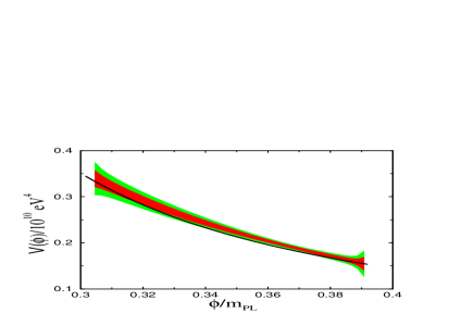
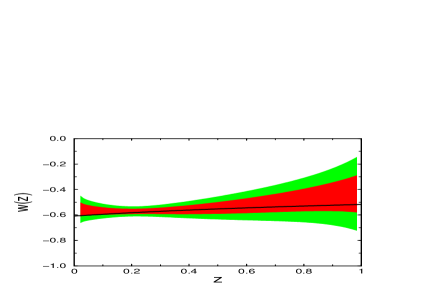
In Fig. 19, we show the simulated reconstruction of the quintessence model with potential $V(\phi)=M^{4}[\exp({m_{\rm Pl}}/{\phi})-1]$ zlatev and $\Omega_{X}=0.50$. We assumed 2000 SNe uniformly distributed out to $z=1.5$ with individual uncertainties of $0.15$ mag. Data were fit by a three-parameter Padé approximant of the form

$$r(z)=\frac{z(1+a\,z)}{1+b\,z+c\,z^{2}}.$$ (37)

We have also tried other fitting functions that have been suggested saini ; chiba2 ; weller , as well as a piecewise cubic spline with variable tension. We find that all are able to fit the predicted form for $r(z)$ well (about 0.2% accuracy). However, a good fit is not the whole story – $r^{\prime}(z)$ and $r^{\prime\prime}(z)$ are equally important – and the small bumps and wiggles between the between the fit and the actual form predicted by the dark-energy model are important because they lead to reconstruction error.

In sum, non-parametric reconstruction is very challenging, and an oxymoron: as a practical matter the data must be fit by a smooth function. Nevertheless, in the absence of a handful of well motivated dark-energy models, reconstruction offers a more general means of getting at the time dependence of $w$ and the very nature of the dark energy. Finally, it goes without saying that the best way to test a specific model is to use it as a representation of the dark energy.

IV.6 Number Counts

Probing $w(z)$ by number counts will involve all the difficulties just discussed for SNe Ia, and the additional issue of separating the evolution of the comoving density of objects (galaxies or clusters) from the cosmological effects of dark energy. To test the probative power of number counts, we consider a cosmological probe that is primarily sensitive to the volume element $dV/dzd\Omega$, such as the galaxy-halo test using the DEEP survey davis . In order to achieve comparable constraints to those provided by SNe Ia, we find that $dV/dzd\Omega$ must be measured to 2-3% in each redshift bin. Even with thousands of halos, the accuracy in the number counts in each redshift bin must be Poisson-limited – a very challenging goal when the ever-present uncertainties in theoretical predictions of abundances of these objects are taken into account.

Figure 20: The 95% cl constraint on $w(z)$ when the dark energy is parameterized by $w_{1}$ and $w^{\prime}$ and the halo counts are divided into 8 redshift bins with $0.7<z<1.5$ (solid lines) and 15 redshift bins with $0<z<1.5$ (dashed lines). The light dotted lines show the result with 8 bins and $0.7<z<1.5$, but now with a 10% (per bin) additional uncertainty due to the evolution.

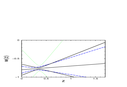
The solid line in Fig. 20 shows the 95% cl constraint on $w(z)$ when this function is parameterized by $w_{1}$ and $w^{\prime}$ for Case I above, with the choice of $z_{1}=0.35$ to decorrelate these two parameters. Two cases were considered, each with a total of 10000 halos. In the first, the objects were binned into 8 redshift bins with $0.7<z<1.5$, as expected for the DEEP sample davis . In the second case, the objects were binned in 15 redshift bins with $0<z<1.5$ (here $z_{1}=0.27$). Filling in the low redshift end improves the constraint.

Finally, we show the constraint to $w(z)$ in the case of 10000 halos with $0.7<z<1.5$, but now assuming that there is a 10% (per bin) additional uncertainty due to the evolution of the comoving number density of halos. The constraint is now considerably weaker, and only $w(z\approx 0.4)$ is determined accurately.

V Optimal Strategies

Here we consider strategies for the most accurate determination of the cosmological parameters, $\Omega_{M}$, $\Omega_{X}$ and the equation-of-state of the dark energy, $w_{X}$, using high-redshift supernovae (we add subscript ’X’ to distinguish it from the weight functions defined below). To this end, we ask, given the cosmological parameters we want to determine, what is the optimal redshfit distribution to best constrain those parameters?

At first glance this problem may appear of purely academic interest since we are not free to put supernovae where we please. However, supernova observers have considerable freedom in choosing redshift ranges for their searches, by using filters sensitive to wavelengths corresponding to spectra at observed redshifts. Moreover, supernovae are easier to discover than follow up, and the answer to the question we pose could well be implemented in the choice of which supernovae are followed up.

In this section we make three assumptions:

(i) Magnitude uncertainty, $\sigma_{m}$, is the same for each supernova irrespective of redshift (this is a pretty good approximation for the current data sets).

(ii) Total number of supernovae observed is fixed (e.g., rather than the total observing time).

(iii) The number of supernovae that can be found at any redshift is not a limiting factor (this is not likely to be a serious consideration).

(iv) For simplicity we assume that type Ia supernovae are standard candles; in fact, they are (at best) standardizable candles whose peak luminosity is related to their rate of decline brightness.

None of these assumptions is required to use the formalism we develop; rather, we make them for concreteness and simplicity. Moreover, any or all of these assumptions can be relaxed with the framework we present. Finally, unless the assumptions prove to be wildly wrong, the results will not change much.

V.1 Preliminaries

We tackle the following problem: given $N$ supernovae and their corresponding uncertainties, what distribution of these supernovae in redshift would enable the most accurate determination of $P$ cosmological parameters? In the case of more than one parameter, we need to define what we mean by “most accurate determination”. Since the uncertainty in measuring $P$ parameters simultaneously is described by an $P$-dimensional ellipsoid (with the assumption that the total likelihood function is Gaussian), we make a simple and, as it turns out, mathematically tractable requirement that the ellipsoid have minimal volume. This corresponds to the best local determination of the parameters.

The volume of the ellipsoid is given by

$$V\propto\det(F)^{-1/2},$$ (38)

where $F$ is the Fisher matrix Fisher-Jungman ; Fisher-Tegmark

$$F_{ij}=-\left<\partial^{2}\ln L\over\partial p_{i}\partial p_{j}\right>_{\bf y},$$ (39)

and $L$ is the likelihood of observing data set ${\bf y}$ given the parameters $p_{1}\ldots p_{P}$. In Appendix A we present the derivation of Eq. (38). To minimize the volume of the uncertainty ellipsoid we must maximize $\det(F)$.

Fisher matrix. The Fisher matrix for supernova measurements was worked out in Ref. CMB+SN ; we briefly review their results, with slightly different notation and one important addition.

The supernova data consist of measurements of the peak apparent magnitude of the individual supernovae, $m_{i}$, which are related to the cosmological parameters by

$$m_{i}=5\log\;[H_{0}d_{L}(z_{n},\Omega_{M},\Omega_{\Lambda})]+{\mathcal{M}}+\epsilon_{i}$$ (40)

where $d_{L}$ is the luminosity distance to the supernova, ${\mathcal{M}}\equiv M-5\log{H_{0}}+25$, $M$ is the absolute magnitude of a type Ia supernova, and $\epsilon_{i}$ is the error in the magnitude measurement (assumed to be Gaussian with zero mean and standard deviation $\sigma_{m}$). Note that ${\mathcal{M}}$ contains all dependence on $H_{0}$, since $d_{L}\propto 1/H_{0}$.

The Fisher matrix is defined as CMB+SN

$$F_{ij}=\frac{1}{\sigma_{m}^{2}}\sum_{n=1}^{N}w_{i}(z_{n})w_{j}(z_{n})$$ (41)

where the $w$’s are weight functions given by

$$w_{i}(z)\equiv{5\over\ln 10}\left\{{\kappa S^{\prime}[\kappa I(z)]\over S[\kappa I(z)]}\left[{\partial I\over\partial p_{i}}-{I(z)\over 2\kappa^{2}}\right]+{1\over 2\kappa^{2}}\right\},$$ (42)

if the parameter $p_{i}$ is $\Omega_{M}$ or $\Omega_{X}$, or else

$$w_{i}(z)\equiv{5\over\ln 10}\left[{\kappa S^{\prime}[\kappa I(z)]\over S[\kappa I(z)]}\,{\partial I\over\partial p_{i}}\right]$$ (43)

if $p_{i}$ is $w_{X}$. Also

$$H_{0}\,d_{L}=(1+z)\,\frac{S(\kappa I)}{\kappa},$$ (44)

$$S(x)=\left\{\begin{array}[]{cl}\sinh(x),&\;\mbox{if}\;\;\Omega_{0}>1;\\ {x},&\;\mbox{if}\;\;\Omega_{0}=1;\\ \sin(x),&\;\mbox{if}\;\;\Omega_{0}<1.\end{array}\right.$$ (45)

$$I(z,\Omega_{M},\Omega_{X},w_{X}) = \int_{0}^{z}H_{0}dx/H(x)$$ (46)

$$\kappa^{2} = 1-\Omega_{M}-\Omega_{X}.$$ (47)

When $w_{X}=-1$ (cosmological constant), we use $\Omega_{\Lambda}$ in place of $\Omega_{X}$.

In addition to $\Omega_{M}$, $\Omega_{X}$ and $w_{X}$, the magnitude-redshift relation also includes the “nuisance parameter” $\mathcal{M}$, which is a combination of the Hubble parameter and absolute magnitude of supernovae, and which has to be marginalized over in order to obtain constraints on the parameters of interest. Ignoring $\mathcal{M}$ (that is, assuming that $\mathcal{M}$ is known) leads to a 10%-30% underestimate of the uncertainties in other parameters. (Of course, accurate knowledge of $H_{0}$ and a large local sample of supernovae could be used to precisely determine $\mathcal{M}$ and eliminate this additional parameter.) For the moment we will ignore $\mathcal{M}$ for clarity; later we will show that it is a simple matter to include $\mathcal{M}$ as an additional parameter which is marginalized over.

The Fisher matrix can be re-written as

$$F_{ij} = {N\over\sigma_{m}^{2}}\int_{0}^{z_{\rm max}}g(z)w_{i}(z)w_{j}(z)dz,$$ (48)

where

$$g(z)={1\over N}\sum_{n=1}^{N}\delta(z-z_{n})$$ (49)

is the (normalized) distribution of redshifts of the data and $z_{\rm max}$ is the highest redshift probed in the survey. [$g(z)$ is essentially a histogram of supernovae which is normalized to have unit area.] Our goal is to find $g(z)$ such that $\det(F)$ is maximal. Note that the maximization of $\det(F)$ will not depend on $N$ and $\sigma_{m}$, so we drop them for now. To consider non-constant error $\sigma_{m}(z)$, one can simply absorb $\sigma_{m}(z)$ into the definition of weight functions $w(z)$.

V.2 Results

One parameter. As a warm-up, consider the case of measuring a single cosmological parameter $p_{1}$. We need to maximize $\int_{0}^{z_{\rm max}}g(z)\,w_{1}^{2}(z)\,dz$, subject to $\int_{0}^{z_{\rm max}}g(z)\,dz=1$ and $g(z)\geq 0$. The solution is a single delta function for $g(z)$ at the redshift where $w_{1}(z)$ has a maximum. For any of our parameters, $w_{1}(z)$ will have a maximum at $z_{\rm max}$. This result is hardly surprising: we have a one-parameter family of curves $m(z)$, and the best way to distinguish between them is to have all measurements at the redshift where the curves differ the most, at $z_{\rm max}$.

Figure 21: Dependence of the magnitude-redshift relation upon the single parameter $\Omega_{M}$, relative to a flat Universe with $\Omega_{M}=0.3$. The maximum difference occurs at the highest redshift.

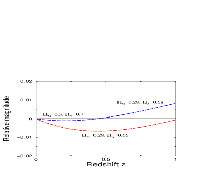
For example, Fig. 21 shows magnitude-redshift curves for the fiducial $\Omega_{M}=0.3$ model with the assumption $\Omega_{\Lambda}=1-\Omega_{M}$ (flat Universe). As $\Omega_{M}$ is varied, the biggest difference in $m(z)$ is at the highest redshift probed. In order to best constrain $\Omega_{M}$, all supernovae should be located at $z_{\rm max}=1.0$,

Two parameters. A more interesting – and relevant – problem is minimizing the area of the error ellipse in the case of two parameters, e.g., $\Omega_{M}$ and $w_{X}$ or $\Omega_{M}$ and $\Omega_{X}$. The expression to maximize is now

$$\int_{z=0}^{z_{\rm max}}g(z)\,w_{1}^{2}(z)dz\int_{z=0}^{z_{\rm max}}g(z)\,w_{2}^{2}(z)dz\;-$$ (50)

$$\left(\int_{z=0}^{z_{\rm max}}g(z)\,w_{1}(z)\,w_{2}(z)dz\right)^{2}$$

$$= {1\over 2}\int_{z_{1}=0}^{z_{\rm max}}\int_{z_{2}=0}^{z_{\rm max}}g(z_{1})\,g(z_{2})\,w(z_{1},z_{2})^{2}\,dz_{1}\,dz_{2},$$

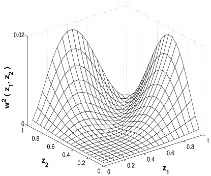
where $w(z_{1},z_{2})\equiv w_{1}(z_{1})w_{2}(z_{2})-w_{1}(z_{2})w_{2}(z_{1})$ is a known function of redshifts and cosmological parameters (see Fig. 22) and $g(z)$ is subject to the same constraints as before.

Figure 22: Top panel: Function $w(z_{1},z_{2})^{2}$ for the case when $\Omega_{M}=0.3$ and $\Omega_{\Lambda}=0.7$. Bottom panel: Dependence of the magnitude-redshift relation upon two parameter, $\Omega_{M}$ and $\Omega_{\Lambda}$, relative to a flat Universe with $\Omega_{M}=0.3$. Observations at more than one redshift are needed to distinguish different models.

Despite the relatively harmless appearance of Eq. (50), we found it impossible to maximize it analytically. Fortunately, it is simple to find the solution numerically. Returning to the discrete version of Eq. (48), we divide the interval $(0,z_{\rm max})$ into $B$ bins with $g_{i}N$ supernovae in bin $i$. We need to maximize

$$\sum_{i,j=1}^{B}g_{i}\,g_{j}\,w(z_{i},z_{j})^{2}$$ (51)

subject to

$$\sum_{i=1}^{B}g_{i}=1\,\,\,\,\,\mbox{and}\,\,\,\,\ g_{i}\geq 0.$$ (52)

Equations (51) and (52) define a quadratic programming problem — extremization of a quadratic function subject to linear constraints. Since $w(z_{1},z_{2})^{2}$ is neither concave nor convex (see Fig. 22), we have to resort to brute force maximization, and consider all possible values of $g_{i}$. The result of this numerical maximization is that the optimal distribution is two delta functions of equal magnitude:

$$g(z)=0.50\;\delta(z-0.43)+0.50\;\delta(z-1.00),$$ (53)

where all constants are accurate to $0.01$. Thus, half of the supernovae should be at the highest available redshift, while the other half at about 2/5 of the maximum redshift.

This result is not very sensitive to the maximum redshift probed, or fiducial parameter values. If we increase the maximum available redshift to $z_{\rm max}=1.5$, we find two delta functions of equal magnitude at $z=0.57$ and $z=1.50$. If we change the fiducial values of parameters to $\Omega_{M}=0.3$ and $\Omega_{\Lambda}=0$ (open Universe), we find delta functions of equal magnitude at $z=0.47$ and $z=1.00$.

For a different choice for the two parameters, $\Omega_{M}$ and $w_{X}$, with fiducial values $\Omega_{M}=0.3$ and $w_{X}=-1$ and with the assumption of flat Universe ($\Omega_{X}=1-\Omega_{M}$). we find a similar result

$$g(z)=0.50\;\delta(z-0.36)+0.50\;\delta(z-1.00).$$ (54)

Three or more parameters. We now consider parameter determination with three parameters $\Omega_{M}$, $\Omega_{X}$ and $w_{X}$. Elements of the $3\times 3$ Fisher matrix are calculated according to Eq. (48), and we again maximize $\det(F)$ as described above. The result is

$$g(z) = 0.33\;\delta(z-0.21)+0.34\;\delta(z-0.64)+$$ (55)

$$0.33\;\delta(z-1.00),$$

with all constants accurate to 0.01. Hence we have three delta functions of equal magnitude, with one of them at the highest available redshift.

We have not succeeded in proving that $P>3$ parameters are best measured if the redshift distribution is $P$ delta functions. However, it is easy to prove that, if the data do form $P$ delta functions, then those delta functions should be of equal magnitude and their locations should be at coordinates where the “total” weight function [e.g. $w(z_{1},z_{2})^{2}$ in case of two parameters] has a global maximum (see Appendix B). In practice, the number of cosmological parameters to be determined from SNe Ia data is between one and three, so considering more than three parameters is less relevant.

Marginalization over $\mathcal{M}$. So far we have been ignoring the parameter $\mathcal{M}$, assuming that it is known (equivalently, that the value of $H_{0}$ and the absolute magnitude of supernovae are precisely known). This, of course, is not necessarily the case, and $\mathcal{M}$ must be marginalized over to obtain probabilities for the cosmological parameters. Fortunately, when $\mathcal{M}$ is properly included, our results change in a predictable and straightforward way.

Including $\mathcal{M}$ as an undetermined parameter, we now have an ($P+1$)-dimensional ellipsoid ($P$ cosmological parameters plus $\mathcal{M}$), and we want to minimize the volume of its projection onto the $P$-dimensional space of cosmological parameters. The equation of the $P$-dimensional projection is

$$X^{T}F_{\rm proj}X=1\,.$$ (56)

$F_{\rm proj}$ is obtained as follows: 1) Invert the original $F$ to obtain the covariance matrix $F^{-1}$;  2) pick the desired $P$x$P$ subset of $F^{-1}$ and call it $F_{\rm proj}^{-1}$;   3) invert it to get $F_{\rm proj}$.

Minimizing the volume of the projected ellipsoid we obtain the result that the optimal supernova distribution is obtained with $P$ delta functions in redshift obtained when ignoring $\mathcal{M}$, plus a delta function at $z=0$. All $P+1$ delta functions have the same magnitude. The explanation is simple: the additional low redshift measurements pin down $\mathcal{M}$.

Redshift dependent $\sigma_{m}$. The optimal redshift distribution changes slightly if the uncertainty in supernova measurements is redshift dependent. Suppose for example that $\sigma_{m}=0.15+\sigma^{\prime}z$, and that $z_{\rm max}=2$. In case of one parameter, the optimal location of SNe starts changing from $z_{\rm max}=2$ only for $\sigma^{\prime}>0.1$, decreasing to $z=1.5$ for $\sigma^{\prime}=0.2$. For the case of two or more parameters, the optimal distribution is even more robust – significant change occurs only for $\sigma^{\prime}\gtrsim 0.3$ in the case of two parameters, and only for $\sigma^{\prime}\gtrsim 1$ in the case of three.

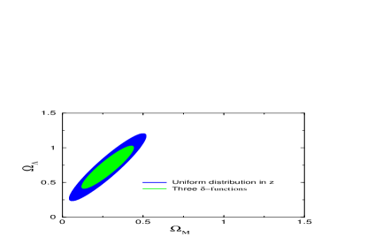
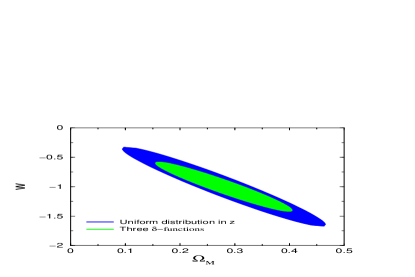
Optimal vs. uniform distribution. Are the advantages of the optimal distribution significant enough that one should consider them seriously? In our opinion the answer is yes, as we illustrate in the top panel of Fig. 23. This figure shows that the area of the $\Omega_{M}$-$\Omega_{\Lambda}$ uncertainty ellipsoid is more than two times smaller if the SNe have the optimal distribution as opposed to uniform distribution. Similar results obtain for other choices of the parameters.

Figure 23: Top and middle panel: Uniform (dark) vs. optimal (light) distribution in redshift. Shown are constraints on $\Omega_{M}$ and $\Omega_{\Lambda}$ (top) and on $\Omega_{M}$ and $w$ for a flat Universe (middle) when $\mathcal{M}$ was marginalized over. For these results, 100 SNe were assumed with individual uncertainties of $\sigma_{m}=0.15$ mag; the size of the error ellipse scales as $\sigma_{m}/\sqrt{N}$. Bottom panel: Thinnest possible ellipse for given $N$ and $\sigma_{m}$ (dark) is infinitely long in one direction. However, the smallest-area ellipse (light) is almost as thin.

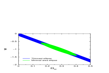
Thinnest ellipse. If we are using SNe Ia alone to determine the cosmological parameters, then we clearly want to minimize the area of the error ellipse. However, supernova measurements will also be combined with other methods to determine cosmological parameters. A good example of the symbiosis is combining CMB measurements with those of supernovae Zaldarriaga ; CMB+SN . These methods together can improve the determination of $\Omega_{M}$ and $\Omega_{\Lambda}$ by up to a factor of 10 as compared to either method alone by breaking the degeneracy between the two parameters. (The improvement is largest when the error ellipses from the two methods are comparable; in the case of SNAP and Planck, the projected SNAP ellipse is so much smaller than Planck only improves parameter determination by 5% to 10%; cf., Fig. 13.)

Finding the thinnest ellipse is a problem that we can solve using our formalism. Since the length of each axis of the ellipse is proportional to the inverse square root of an eigenvalue of the corresponding Fisher matrix, all we need to do is maximize the larger eigenvalue of $F$ with respect to the distribution of the supernovae $g(z)$.

The result is perhaps not surprising: to get the thinnest ellipse, all supernova measurements should be at the same (maximum) redshift, which leads to an infinitely long ellipse. We find that changing the supernovae redshift distribution doesn’t change the width of the error ellipse greatly, but does change its length. As a practical matter, we find the smallest area ellipse is very close to being the thinnest ellipse (see bottom panel of Fig. 23).

Reconstruction. In the spirit of our analyses above, we ask: what redshift distribution of supernovae gives the smallest 95% confidence region for the reconstructed quintessence potential $V(\phi)$? To answer this question, we perform a Monte-Carlo simulation by using different distributions of supernovae and computing the average area of the confidence region corresponding to each of them.

Uniform distribution of supernovae gives the best result among the several distributions we put to test. This is not surprising, because reconstruction of the potential consists in taking first and second derivatives of the distance-redshift curve, and the most accurate derivatives are obtained if the points are distributed uniformly. For comparison, Gaussian distribution of supernovae with mean $\overline{z}=0.7$ and spread $\sigma_{z}=0.4$ gives the area that is $10-20$% larger.

VI Conclusions

Determining the nature of the dark energy that accounts for 2/3rds of the matter/energy in the Universe and is causing its expansion to accelerate ranks as one of the most important problems in both physics and astronomy. At the moment, there is very little theoretical guidance, and additional experimental constraints are urgently needed. Because of its diffuse nature, the effect of dark energy on the large-scale dynamics of the Universe offers the most promising way to get this empirical information.

The first step is to determine the average equation-of-state of the dark energy. CMB anisotropy, supernovae distance measurements and number counts all appear promising. The Alcock-Paczynski shape test and the age of the Universe seem somewhat less promising; the former because of the small size of the effect (around 5%); and the latter because the errors in the two needed quantities, $H_{0}$ and $t_{0}$, are not likely to become small enough in the near future.

The main sensitivity of the CMB to the dark energy is the $w$ dependence of the distance to the surface of last scattering, which moves the positions of the acoustic peaks in the angular power spectrum. The CMB is much more sensitive to $\Omega_{0}$ than $w$, and the ultimate sensitivity of the CMB anisotropy to $w$ will come from Planck, $\sigma_{w}\simeq 0.25$.

Probes of the low-redshift Universe (supernovae and number counts) seem more promising. In contrast to the CMB, they only depend upon three cosmological parameters ($\Omega_{M}$, $\Omega_{X}$ and $w$), which will be effectively reduced to two ($\Omega_{X}$ and $w$) when precision CMB measurements determine $\Omega_{0}=\Omega_{M}+\Omega_{X}$ to better than 1%. They are most sensitive to $w$ between $z\sim 0.2$ and $z\sim 2$ (with “sweet spot” at $z\simeq 0.4$).

A high-quality sample of 2000 supernovae out to redshift $z\sim 1.5$ could determine $w$ to a precision of $\sigma_{w}=0.05$ (or better if the optimal redshift distribution is achieved), provided that the systematics associated with type Ia supernovae can be controlled (e.g., luminosity evolution, photometric errors, and dust). A similar accuracy might be achieved by number counts of galaxies out to $z\sim 1.5$ or of clusters of galaxies. The critical ingredient is understanding (or independently measuring) the evolution of the comoving number density (in the case of galaxies to be better than 5%).

More difficult, but very important, is a determination of, or constraint to, the time variation of $w$. If $w(z)$ is parameterized to vary linearly (or logarithmically) with redshift, and assuming perfect knowledge of $\Omega_{M}$ and $\Omega_{X}$, a precision $\sigma_{w^{\prime}}\simeq 0.16$ might be achieved by supernova distance measurements ($w^{\prime}=dw/dz$). However, uncertainty in $\Omega_{M}$ significantly degrades $\sigma_{w^{\prime}}$ (see Fig. 16).

Non-parametric reconstruction of either $w(z)$ or the potential-energy curve for a quintessence model is the most demanding test, as it requires the first and second derivatives of the luminosity distance $d_{L}$. Even very accurate measurements of $d_{L}$ cannot constrain the small bumps and wiggles which are crucial to reconstruction. Without some smoothing of the cosmological measurements, reconstruction is impractical. (The combination of number counts and supernova measurements could determine $H(z)$ directly and eliminate the dependence upon the second derivative of $d_{L}$.)

We have not addressed systematic error in any detail, and for this reason our error forecasts could be very optimistic. On the other hand, the number of supernovae measured could be larger and the uncertainties could be smaller than assumed (in general, our error estimates scale as $\sigma_{m}/\sqrt{N}$).

We are at a very early stage in the study of dark energy. Ways of probing the dark energy not discussed here could well prove to be equally or even more important. Four examples come to mind. First, the existence of a compelling model (or even one or two-parameter class of models) would make the testing much easier, as the predictions for $d_{L}(z)$ and other cosmological observables could be directly compared to observations. Second, we have shown that one of the most powerful cosmological probes, CMB anisotropy, has little leverage because dark energy was unimportant at the time CMB anisotropies were formed ($z\sim 1100$). Interesting ideas are now being discussed where the ratio of dark energy to the total energy density does not decrease dramatically with increasing redshift (or even stays roughly constant) manojetal ; aaetal ; if correct, the power of the CMB as a dark energy probe could be much greater. Third, we have assumed that the slight clumping of dark energy on large scales is not an important probe. While there are presently no models where dark energy clumps significantly, if it does (or if the clumping extends to smaller scales) CMB anisotropy and large-scale structure measurements might have additional leverage. Finally, it is possible that dark energy leads to other observable effects such as a new long range force.

Appendix A proof of equation (38)

To derive Eq.  (38), consider a general uncertainty ellipsoid in $n$-dimensional parameter space. The equation of this ellipsoid is

$$X^{T}FX=1,$$ (57)

where $X=(x_{1}x_{2}\ldots x_{P})$ is the vector of coordinates and $F$ the Fisher matrix. Let us now choose coordinates so that the ellipsoid has its axes parallel to the new coordinate axes. Here $X_{\rm rot}=UX$, where $U$ is the orthogonal matrix corresponding to this rotation. The equation of the ellipsoid in the new coordinate system is

$$X_{\rm rot}^{T}\,F_{\rm rot}\,X_{\rm rot}=1,$$ (58)

where $F_{\rm rot}=UFU^{T}$ is the Fisher matrix for the rotated ellipsoid, and has the form $F_{\rm rot}=diag(1/\sigma_{1}^{2},\ldots,1/\sigma_{P}^{2})$. The volume of the ellipsoid is just

$$V\propto\prod_{i=1}^{P}\sigma_{i}=\det(F_{\rm rot})^{-1/2}.$$ (59)

Then, since $\det(F)=\det(F_{\rm rot})$ and rotations preserve volumes, we have

$$V\propto\det(F_{\rm rot})^{-1/2}=\det(F)^{-1/2}.$$ (60)

This completes the proof.

Appendix B Measuring $P$ parameters

We first prove the following: if we want to determine $P$ parameters by having measurements that form $P$ delta functions in redshift (we have shown this is optimal for $P=1,2,3$ in Sec. V.2), then those delta functions should be of equal magnitude. The distribution of measurements is

$$g(z)=\sum_{i=1}^{P}\alpha_{i}\;\delta(z-z_{i})$$ (61)

with

$$\sum_{i=1}^{P}\,\alpha_{i}=1.$$ (62)

We need to maximize

$$\det F\propto\int g(x_{1})\ldots g(x_{P})\,W(x_{1},\ldots x_{P})\,dx_{1}\,\ldots dx_{P}$$ (63)

where $x$’s are dummy variables and all integrations run from $0$ to $z_{\rm max}$. Here $W$ is given in terms of weight functions $w_{i}$, and is symmetric under exchange of any two arguments and zero if any two arguments are the same. Then only one term in the integrand of (63) is non-zero and that expression simplifies to

$$\det F\propto\,P!\;\alpha_{1}\ldots\alpha_{P}\,W(z_{1},\ldots z_{P}).$$ (64)

From (62) and (64) one easily shows that $\det F$ is maximized if $W$ has maximum at $(z_{1},\ldots,z_{P})$ and $\alpha_{1}=\alpha_{2}=\ldots=\alpha_{P}=1/P$. Therefore, the delta functions must be of equal magnitude, and located where $W$ has its global maximum.

References

- (1) S. Perlmutter et al., Astrophys. J. 517, 565 (1999)
- (2) A. Riess et al., Astron. J. 116, 1009 (1998)
- (3) M. S. Turner, in Type Ia Supernovae: Theory and Cosmology, eds. J. C. Niemeyer and J. W. Truran (Cambridge University Press, Cambridge, UK), p. 101
- (4) S. Dodelson and L. Knox, Phys. Rev. Lett. 84, 3523 (2000)
- (5) P. de Bernardis et al., Nature 404, 955 (2000)
- (6) A. Balbi et al., astro-ph/0005124
- (7) A.H. Jaffe et al., astro-ph/0007333
- (8) M. S. Turner, Physica Scripta T85, 210 (2000)
- (9) M.S. Turner, in Proceedings of Type Ia Supernovae: Theory and Cosmology (Chicago, October 1998), eds. J.C. Niemeyer and J.W. Truran (Cambridge Univ. Press, Cambridge, UK, 2000), p. 101 (astro-ph/9904049)
- (10) See e.g., S. Dodelson et al, Science 274, 69 (1996); L. Krauss and M.S. Turner, Gen. Rel. Grav. 27, 1137 (1995); J.P. Ostriker and P.J. Steinhardt, Nature 377, 600 (1995); J. Colberg et al, Mon. Not. R. astron. Soc. 319, 209 (2000).
- (11) S. Weinberg, Rev. Mod. Phys. 61, 1 (1989)
- (12) M. Bronstein, Phys. Zeit. Sowjet Union 3, 73 (1933); M. Ozer and M.O. Taha, Nucl. Phys. B 287 776 (1987); K. Freese et al., ibid 287 797 (1987); L.F. Bloomfield-Torres and I. Waga, Mon. Not. R. astron. Soc. 279, 712 (1996); J. Frieman et al, Phys. Rev. Lett. 75, 2077 (1995); B. Ratra and P. J. E. Peebles, Phys. Rev. D 37, 3406 (1988); P. G. Ferreira and M. Joyce, Phys. Rev. D 58, 023503 (1998); R. Caldwell, R. Dave, and P.J. Steinhardt, Phys. Rev. Lett. 80, 1582 (1998)
- (13) I. Zlatev, L. Wang and P. J. Steinhardt, Phys. Rev. Lett. 82, 896 (1999)
- (14) S. Dodelson, M. Kaplinghat, and E. Stewart, Phys. Rev. Lett., in press (2001) (astro-ph/0002360)
- (15) C. Skordis and A. Albrecht, astro-ph/0012195.
- (16) C. Armendariz-Picon, V. Mukhanov and P.J. Steinhardt, astro-ph/0006373
- (17) A. Vilenkin, Phys. Rev. Lett. 53, 1016 (1984); D. Spergel and U.-L. Pen, Astrophys. J. 491, L67 (1997); A. Vilenkin and E. P. S. Shellard, Cosmic strings and other topological defects (Cambridge Univ. Press, Cambridge, UK, 1994)
- (18) M. S. Turner and F. Wilczek, Nature 298, 633 (1982)
- (19) N. Arkani-Hamed et al., Phys. Lett. B 480, 193 (2000)
- (20) L. Parker and A. Raval, Phys. Rev. D 62, 083503 (2000)
- (21) G.W. Anderson and S.M. Carroll, “Dark Matter with Time-Dependent Mass,” in Cosmo-97, International Workshop on Particle Physics and the Early Universe, ed. L. Roszkowski (World Scientific: Singapore), p. 227 (1997), astro-ph/9711288
- (22) M. Bucher and D. N. Spergel, Phys. Rev. D 60, 043505 (1999)
- (23) W. Hu, Astrophys. J. 506, 485 (1998)
- (24) B. Ratra and P. J. E. Peebles, Phys. Rev. D 37, 3406 (1988); K. Coble, S. Dodelson, and J. Frieman, Phys. Rev. D 55, 1851 (1996); R. Caldwell, R. Dave, and P.J. Steinhardt, Phys. Rev. Lett. 80, 1582 (1998)
- (25) M. S. Turner and M. White, Phys. Rev. D, 56, R4439 (1997)
- (26) S. M. Carroll, Phys. Rev. Lett. 81, 3067 (1998)
- (27) http://snap.lbl.gov
- (28) I. Maor, R. Brustein, and P. J. Steinhardt, astro-ph/0007297
- (29) S. Podariu, P. Nugent and B. Ratra, astro-ph/0008281
- (30) J. Weller and A. Albrecht, astro-ph/0008314
- (31) P. Astier, astro-ph/0008306
- (32) Cosmological strategies for getting at the nature of a smooth cosmological component were first addressed by J. C. Charlton and M. S. Turner, Astrophys. J. 313, 495 (1987)
- (33) See e.g., W. Freedman, Phys. Repts. 333-334, 13 (2000) and L. Krauss, ibid, 33 (2000).
- (34) X. Fan, N. A. Bahcall and R. Cen, Astrophys J. 490, L123 (1997)
- (35) W. H. Press and P. L. Schechter, Astrophys. J. 187, 425 (1974)
- (36) C.S. Kochanek, Astrophys. J. 466, 638 (1996); W. Hu and M. Tegmark, Astrophys. J. 514, L65 (1999); J.A. Tyson, D. Wittman and J.R.P. Angel, astro-ph/0005381
- (37) See e.g., P.T.P. Viana and A.R. Liddle, Mon. Not. R. astron. Soc. 303, 535 (1999)
- (38) C. Alcock and B. Paczynski, Nature 281, 358 (1979)
- (39) W. Ballinger, J.A. Peacock and A.F. Heavens, Mon. Not. R. astron. Soc. 282, 877 (1996)
- (40) L. Hui, A. Stebbins and S. Burles, Astrophys. J. 511, L5 (1999); P. McDonald and J. Miralda-Escude, ibid 518, 24 (1999); M. Davis, talk at Pritzker Symposium (Chicago, January 1999).
- (41) W. Hu and N. Sugiyama, Astrophys. J. 444, 489 (1995)
- (42) U. Seljak and M. Zaldarriaga, Astrophys. J. 469, 437 (1996)
- (43) S. Weinberg, astro-ph/0006276
- (44) D. Huterer and M.S. Turner, Phys. Rev. D 60, 081301 (1999)
- (45) S. Perlmutter, M.S. Turner and M. White, Phys. Rev. Lett. 83, 670 (1999)
- (46) G. Aldering et al., Supernova Factory Webpage (http://snfactory.lbl.gov)
- (47) M. Davis and J. Newman, Astrophys J. 513 , L95 (1999)
- (48) G. Holder, Ph.D. thesis (2001).
- (49) Z. Haiman, J. J. Mohr, and G. P. Holder, astro-ph/0002336
- (50) P. M. Garnavich et al, Astrophys. J. 509, 74 (1998)
- (51) W. Hu et al, Phys. Rev. D. 59, 023512 (1998)
- (52) K. Coble, S. Dodelson, and J. Frieman, Phys. Rev. D 55, 1851 (1996)
- (53) A. R. Cooray and D. Huterer, Astrophys. J., 513, L95 (1999)
- (54) D. Eisenstein, W. Hu, M. Tegmark, Astrophys. J. 518, 2 (1999)
- (55) D. Eisenstein, private communication
- (56) G. Efstathiou, Mon. Not. R. astron. Soc. 310, 842 (1999)
- (57) T. Chiba and T. Nakamura, Mon. Not. R. astron. Soc. 306, 696 (1999)
- (58) T. D. Saini et al, Phys. Rev. Lett. 85, 1162 (2000)
- (59) T. Nakamura and T. Chiba, astro-ph/0008175
- (60) G. Jungman et al, Phys. Rev. D 54, 1332 (1996)
- (61) M. Tegmark, A. N. Taylor, and A. F. Heavens, Astrophys. J. 480, 22 (1997)
- (62) M. Tegmark et al, astro-ph/9805117
- (63) M. Zaldarriaga, D. N. Spergel, U. Seljak, Astrophys. J. 488, 1 (1997)
- (64) J. C. G. Boot, Quadratic Programming: Algorithms, Anomalies [and] Applications (North-Holland, Amsterdam 1964)