Demographics of Blazars

Abstract

We discuss the preliminary results of an extensive effort to address the fundamental, and yet un-answered, question that can be trivialized as: “are there more blue or red blazars?”. This problematic is tightly connected with the much debated issue of the unified picture(s) of radio–loud AGNs, which in turn revolves around the existence, and the properties of relativistic jets. We address this question by comparing –simultaneously– the properties of the collection of heterogeneously selected samples that are available now, with the predictions of a set of plausible unifications scenarios. We show that it is already possible to make significant progress even by using only the present samples. The important role of selection effects is discussed. For instance we show that the multiple flux selections typical of available surveys could induce some of the correlations found in color–color diagrams. These latter results should apply to any study of flux limited samples.

University of California at San Diego, Center for Astrophysics and Space Sciences, 9500 Gilman Drive, La Jolla, CA 92093-0424, USA

1. The factor of 100 problem

More than 95% of all catalogued blazars have been found in either shallow radio or shallow X-ray surveys (e.g. see Padovani, these proceedings). Because of the range of blazar spectral energy distributions (SED) the two selection methods yield different types, the “red” objects (with the peak of the synchrotron emission at IR-optical wavelengths, LBL) in radio samples, and the “blue” (whose synchrotron emission peaks at UV-X-ray wavelengths, HBL) in X-ray samples. The differences in the SEDs do reflect different physical states but only as the extrema of an underlying continuous population.

The relative space densities of the different types, not to mention their absolute space densities or their evolution in cosmic time still remain indeterminate. Different scenarios predict a difference of two orders of magnitude (!) in the ratio of the “red” and “blue” types, nevertheless the presently available samples are unable to distinguish between them. The blazar demographics are this uncertain essentially because the flux limits of current complete samples are high, so only the tip of the population is sampled. The interpretation of observed phenomenology depends on the complicated sensitivity of diverse surveys to a range of spectral types. Ultimately, this means we do not know which kind of jets nature preferentially makes: those with and high $B$ and $\gamma_{\rm e}$ (“blue” blazars) or low $B$ and $\gamma_{\rm e}$ (“red” blazars). We also do not know whether they evolve differently and/or if “red” blazars dominate at high redshift and evolve into “blue” blazars at low redshift, and what is the relationship between the “non-thermal” and “thermal” power/components. The implications for understanding jet formation are obvious.

Here we present a concise account of the preliminary results of numerical simulations of a set of unification models, including an actual fit of the model parameters to reproduce the general characteristics of a few reference samples (§2). We also introduce a “concept” experiment, devised to address the role of selection effects (§3), and discuss a couple of issues that are connected to this problem. In §4 we comment on future developments.

2. Testing unification scenarios

We compared the existing surveys with a set of three alternative unified schemes, following the discussion developed in recent years after Padovani & Giommi (1995), and Fossati et al. (1997, 1998). They are: i) the “radio–leading”, where the primary luminosity is the radio one and N${}_{\rm LBL}>$N_HBL. ii) The “X–ray-leading”, where the primary band are the X–ray, and N${}_{\rm LBL}<$N_HBL. iii) The “bolometric”, where the SED properties (and in turn the distribution of L_X/L_R, i.e. the balance between LBL and HBL) are determined by the total power of the source, with HBLs being the less powerful objects. In Fossati et al. (1997) the input parameters of each model were pre-set to values based on those of the observed samples. The most interesting results was the success of the new model, the bolometric one.

Figure 1.: Evolution during the fit of the values of (a) $\chi^{2}$ and (b) of the width $\sigma$ of the L–$\nu_{\rm peak}$ relationship for the bolometric model. In (c) is plotted the area of the “LBL Gaussian” for the radio–leading model.

2.1. The fit method, and results

In this work our approach is different. First we normalize/optimize each unifying scheme by performing an actual fit to three reference samples (EMSS, Slew, 1 Jy). We leave free to vary 7–8 variables, such as the normalization and slope of the primary luminosity function, and the distribution of the L_X/L_R ratio. For those parameter for which there is a measured value (e.g. the luminosity function) we allowed their values to move within their 2$\sigma$ interval. The observational quantities to reproduce were the number, and average radio and X–ray luminosities of HBLs and LBLs.

The technique used for the fit is “simulated annealing” (e.g. Kirkpatrick et al. 1983), which is based on statistical mechanics, and implemented via MonteCarlo. It is a very robust technique, very well suited for many parameter fits. Moreover the “global” nature of the technique is very effective for cases where there might be multiple secondary local minima in the parameter space.

In Fig. 1 we show examples of the evolution of the fit. We here just point out interesting results concerning two of the “core” issues: i) the best fit of the bolometric model requires a finite width for the L–$\nu_{\rm peak}$ relationship (see Fig. 1b). The best fit value is $\sigma\simeq 0.6$, i.e. at any given L the synchrotron peak frequency will be distributed as a Gaussian of width $\sigma$ centered at the $\nu_{\rm peak}$ value determined by the relationship. ii) In both the radio– and X–ray (not shown) leading cases the best fit L_X/L_R distribution is basically a single, broad, Gaussian (see Fig. 1c). For the radio–leading case the LBL Gaussian comprises 98% of the total area, and it is centered at $\simeq-6.3$ with $\sigma\simeq 0.6$.

      

Figure 2.: Radio log(N)-log(S) predicted by the (a) bolometric and the (b) radio-leading models for the DXRBS sample. (c) Bolometric and radio–leading predictions for the “sedentary” sample; the grey-filled square represents the observed density.

2.2. Comparison with real samples

The next step is to use the results of the fits to predict the properties of samples that have not been used to optimize the parameters of the models. We present here only the integral log(N)–log(S) curves, and we only sub-divide the samples in HBL/LBL (according to the values of F_X/F_R). It is worth noting that the absolute normalizations may not be completely reliable, because of uncertainties on the sky coverage. The uncertainty on the (details of) sky coverage is indeed probably the main one involved in the simulations. The relative fraction of HBL and LBL may be a more robust parameter, and it is the one more easily amenable to a quick comparison.

DXRBS

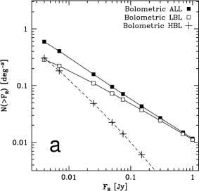
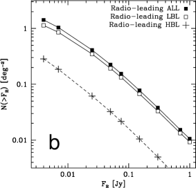
The DXRBS sample (Perlman et al. 1998) is still in progress, but an “off record” comparison of the predicted log(N)–log(S) (shown if Fig. 2a,b) with the observed one seems to show that the models are (still) in good agreement with the data. The predictions of the bolometric and radio–leading models become radically different below about 100 mJy, a domain now reachable. The LBL/HBL density ratio at a few radio flux limits are the following:

      Flux @5GHz      Bolometric  X-ray leading  Radio-leading
        @300 mJy          9.7          6.9            6.6
        @150 mJy          6.2          5.7            6.4
         @50 mJy          3.2          5.2            6.1

Sedentary survey

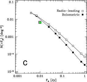
The “sedentary” sample (Giommi, Menna & Padovani 1999) comprises only HBLs because of the built–in cut in $\alpha_{\rm RX}$. The radio log(N)–log(S) is shown in Fig. 2c, where the grey square represent a density @10 mJy between the actual “sedentary” and the EMSS, showing that there is a quite good agreement. Here, as for the DXRBS, we do not plot the predictions of the X–ray leading model because they are not satisfactory. In fact this scenario does not seem to be able to explain the properties of these recent samples, at least with its parameters set at the best fit values.

           

Figure 3.: Radio log(N)–log(S) predicted by the bolometric/radio–/X–ray-leading models: HBLs and LBLs for a sample with an additional cut at (a) m${}_{\rm V}<$20, or (b) m${}_{\rm V}<$22 .

2.3. Going deeper

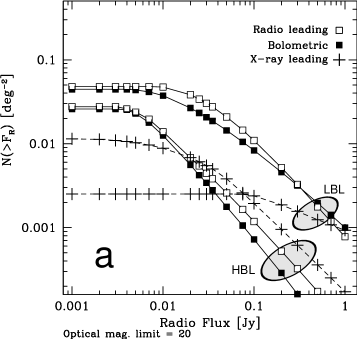
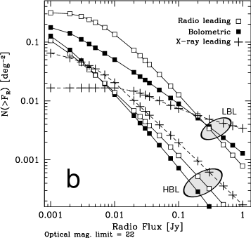
In Fig. 3a,b we show the predictions of the 3 scenarios for the number densities of HBLs and LBLs in radio surveys with a secondary cut in optical magnitude at m_V=20, and m_V=22. We see that the X–ray leading model is giving a substantially different answer from the two other competing models, which seem to agree over most of the accessible radio flux range. The bolometric and radio–leading models actually start to give different predictions only at very faint radio fluxes, as seen in Fig. 3b. In the radio–leading model the radio counts of HBLs and LBLs keep a fixed ratio by definition, while in the bolometric picture HBLs are deemed to eventually outnumber the LBLs, but this seems to happen at radio fluxes lower that expected. However, we are not far from the range of radio fluxes that will be the most sensitive to discriminate among the different pictures. Actually there are already a few samples going deep enough.

2.4. The “cube” (caveat #1)

To try to assess the problem of selection effects we introduced the “cube”. (Fossati & Urry, in preparation), a toy model stripped down of every a priori assumption as to the presumed intrinsic properties of the SED. We assume that the radio/optical/X–ray luminosities are completely un-correlated, and we take simple power law luminosity functions. We then simulate samples of sources that would be selected by a generic flux limited radio or X–ray survey (including the flux dependent sky coverage), with a possible additional cut in another spectral band. An example of the results of this exercise is shown in Fig 4a. It seems to be relatively “natural” to obtain patterns in a color–color diagram which looks like those that are actually observed, and promptly interpreted as tracing intrinsic properties of the sources. Of course the “cube” is not able to reproduce the large variety of patterns and correlations observed in luminosity–luminosity, color–color diagrams, nevertheless we regard it as a very instructive example of how careful we need to be when dealing with selection effects.

             

Figure 4.: (a) $\alpha_{\rm RO}$ vs. $\alpha_{\rm OX}$ diagram with the density contours predicted by the “cube” for an EMSS–like (dotted), a DXRBS–like (dashed), and a radio (solid) selected samples. (b) “Observed” (empty symbols) and “intrinsic” (filled) log(N)–log(S) of extreme HBLs.

2.5. Caveat #2: on cutting in F_X/F_R color

Figure 4b shows the log(N)–log(S) of observed extreme HBL (lower dashed line) and of intrinsic extreme HBL (upper solid line), defined as such according to the observed or intrinsic X–ray/radio ratio. Because of the K–correction and their SED shape, blazars systematically shift towards the LBL side when seen at higher redshift, when “classified” on the basis of the observed X/radio ratio. The effect can be sensible when comparing relative populations of HBL and LBL.

3. Conclusions: blazars demographics and not–so–perfect samples

On the basis of the analysis presented here, we think that there might be already enough information available to proceed to constrain meaningfully the main features of unified scenarios. The comparison of observed samples with simulations performed in a systematic fashion (e.g. by means of simultaneous fit) may provide an extremely powerful and effective tool to address the problem of the intrinsic properties of blazars.

In fact, although there is not a single sample comprising all the desirable characteristics to provide the least possible biased picture of the intrinsic properties of blazars, the F_X/F_R plane is now well covered (see Fig. 1, 2 in Padovani’s contribution). Moreover, the quality of the most recent samples will allow to compare the predictions and the data directly by using the distribution of the $\alpha_{\rm RX}$, an important step forward and past some confusion created by selection effects combined with the “two bins” approach (e.g. §2.5).

If the selection biases of each of surveys can be regarded as being under control (and therefore reliably implemented in the simulations) we may soon be able not only to test a given unified scheme, but even to derive directly from the data what should be the general properties of a successful unified scheme.

Finally, we think that more than ever it is necessary to shift the focus away from the BL Lacs sub-class, because this could still be the source of significant confusion. The best progress could be made by considering the BL Lacs–FSRQs relationship as a whole, also from the observational point of view. The bolometric scenario was meant from the beginning to unify BL Lacs and FSRQs, and it tries to connect some basic physical ideas to the observed phenomenology. On the other hand we need to figure out how to explain the HBL/LBL ratios assumed by the radio and X–ray leading scenarios, and in turn how to extend these models to include smoothly the FSRQs. There should be a way to tell from “first principles” on which side of the 1/10–10/1 range the real value of N_HBL/N_LBL ratio is more likely to belong.

Acknowledgments.

I’d like to thank the organizers for a great workshop, and for bearing with my request of delaying my talk by one day, and Ilaria Cagnoni for very kindly accepting to swap our talks in the schedule. I also thank pippol for the neverending support.

References

Fossati, G. et al. 1997, MNRAS, 289, 136

Fossati, G. et al. 1998, MNRAS, 299, 433

Giommi, P., Menna, M.T., & Padovani, P. 1999, MNRAS, 310, 465

Kirkpatrick, S. et al. 1983, Science, 220, 671

Padovani, P., & Giommi, P. 1995, ApJ, 444, 567

Perlman, E., et al. 1998, AJ, 115, 1253