Issues and methods for CMB anisotropy data reduction
Abstract
Major issues and existing methods for the reduction of CMB anisotropy data are reviewed. An emphasis is put on the importance of proper modelling of the data. It is suggested that the robustness of methods could be improved by taking into account the uncertainty of the model for finding optimal solutions.
keywords:
methods: data analysis, methods: numerical, cosmology: cosmic microwave backgroundPACS:
98.80-k,98.70.Vc,95.75-z,95.75.Pq1 Introduction
The importance of measuring anisotropies of the Cosmic Microwave Background (CMB) to constrain cosmological models is now well established. It has been demonstrated that the properties of these anisotropies depend drastically on the seeds for structure formation as well as on cosmological parameters describing the matter content, the geometry, and the evolution of our Universe [1, 2].
The complexity of CMB data taking into account imperfections in the observations, however, has led the CMB community into developing sophisticated data reduction methods. In this review paper, I discuss the principal issues about CMB data analysis, centering the discussion on map-making, as other aspects related to estimation and its interpretation are discussed by other authors in these proceedings.
2 Modelling the data for its reduction
Data reduction methods involve:
-
•
writing down an accurate model of the problem (including prior knowledge);
-
•
deciding optimisation criteria;
-
•
finding the optimal solution given the model and the optimisation criteria;
-
•
implementing the solution numerically.
The last two aspects have been discussed extensively in the litterature in the context of CMB anisotropy measurements [3, 4]. Less emphasis has been put on the first two aspects so far, although they are certainly as important as the last two.
modelling
For most CMB experiments, the problem is modelled as trying to measure CMB temperature fluctuations of the sky in a number of sky pixels, indexed here by , having measurements in the form of a series of samples (in the context of map-making, for instance, samples can typically be indexed by time). The simplest way of expressing the measurements as a function of the unknown is:
| (1) |
here, and are one-dimensional vectors indexed by pixel numbers and by time. is a pointing matrix telling how much of pixel is seen at time . is the noise. Summation over repeated indices is assumed.
If we have several timelines corresponding to several detectors, the measurement can be modelled as one single data vector by appending all data streams one after the other. Similarly, when the sky emission, represented by temperature is a superposition of emissions due to various astrophysical processes, the system can be written in the form of equation 1 with indexing both pixel and component (instead of pixel only). If there are components (galactic dust, CMB, Sunyaev Zel’dovich emission,…), the linear system becomes simply times as large (with times more unkowns). Formulation 1 is thus quite general (up to the constraint that the model is linear).
It is often assumed that the pointing matrix is perfectly well known, that the noise is Gaussian (and stationnary) and that its autocorrelation (the so-called noise covariance matrix) is known ( is the transpose of vector ).
Optimisation criteria
The “Optimisation” of the processing requires an optimisation criterium. For the construction of a pixellised map one wants typically to minimise the quadratic sum of the errors in all pixels:
| (2) |
where denotes the estimator of the true pixel temperature . If the distributions for and are Gaussian and their autocorrelations and are known, minimising the of equation 2 leads to the Wiener solution:
| (3) |
Alternatively, assuming no prior knowledge on the sky signal, one may decide to minimize a standard on the measurements:
| (4) |
in which case the solution is the COBE method, i.e.:
| (5) |
The Wiener method is the optimal linear method when all processes are Gaussian and when their spectra are known. Non-linear methods relying on Maximum Entropy, using Neural Networks, or linear methods using wavelets may perform better in a variety of cases [5, 6, 7].
Both the Wiener and the COBE methods rely on a particular prior knowledge about the signal and the noise: the knowledge of their autocovariance. The availability of such prior information is far from being obvious, as stressed by Ferreira and Jaffe [8], even if it does not need to be perfect.
The results of the data reduction depend to some extent on the reliability of this knowledge. If we assume that the noise is white (uncorrelated), for instance, the COBE method reduces to simple averaging of measurements in pixels:
| (6) |
If the assumption is erroneous (i.e. the noise is not white), this map-making method is very far from being optimal [4, 9].
More generally, the results of the data reduction depend on the accuracy of the model. In the future, methods taking into account explicitely the confidence one has in the model should be implemented. This is the object of current research. I believe it will help finding the best solution, as well as quantifying the errors, making results more robust.
Optimal solution
Once the problem is properly modelled, finding the optimal mathematical solution to data reduction is generally not the most difficult task for the applications we are interested in. The assesment of errors in the case of non gaussian processes, however, is not simple. So far, linear methods with the assumption of Gaussianity have performed satisfactorily.
Implementation
The numerical implementation of even the simplest data reduction scheme is quite a formidable problem in the context of present and future CMB missions, as emphasised by Bond et al. [10]. Iterative methods to solve large systems can be employed in some cases [3], but implementing the optimal solution for a large and complex system as for the upcoming Planck mission is a hard task.
3 Main issues for data reduction and interpretation
We now review and discuss specific examples which constitute some of the major issues about CMB observation and data analysis:
-
1.
astrophysical foregrounds
-
2.
noise and slow drifts (the so-called 1/f noise)
-
3.
imperfections of instrument properties and of their knowledge
Astrophysical components
CMB anisotropy experiments observe the sky at frequencies ranging from few GHz to few hundreds of GHz, at centimeter to millimeter wavelengths. The observed emission is not only due to CMB anisotropies, as other astrophysical processes also emit in this frequency range [11]. The major known contributors are three galactic processes (thermal galactic dust emission, bremsstrahlung emission of free electrons – the so-called free-free emission, synchrotron emission) and extragalactic sources (IR and radio galaxies, and hot ionised gaz through the SZ effect, principally in clusters of galaxies). In data processing, one needs to separate the contribution of different sources. This aspect will be discussed in section 4.
Noise and slow drifts
The presence of slow drifts in the data streams is a well known problem to CMB anisotropy measurements. Long-term instabilities is a particularity of the sensitive detector technology used for CMB mapping. Such instabilities originate in a combination of detector 1/f noise, thermal instabilities, amplifier gain instabilities, fluctuations of atmospheric emission (especially for ground-based experiments). For radio detectors with HEMT amplifiers, the main source of slow drifts is 1/f noise. For bolometers, it is more often thermal fluctuations of the detector environment that causes trouble. For instance, a 3% emissive telescope mirror which temperature fluctuates by 0.1 K generates 3 mK fluctuations in detected signals, which is mainly in the form of random low-frequency drifts. Removing the effects of such slow drifts is known as “destriping”, and will be discussed in section 5.
Imperfections of a real instrument
Departures from ideality in the instruments must be taken into account. This is especially the case for sensitive experiments as Planck, for which it is targetted to measure the fluctuation power spectrum down to one per cent accuracies per single value.
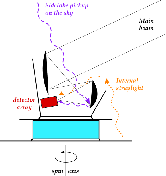
One critical aspect for Planck is the problem of straylight, which is the unwanted radiation received by the instrument detectors. Straylight can be divided into two broad categories. The first one is straylight originating in the sidelobe pickup of astrophysical radiation outside the line of sight defined by the detectors main beams. This problem of “sidelobe straylight” is well known to telecommunication engineers as well as radio-astronomers. The second, more specific to CMB anisotropies (especially at high frequency) is that of straylight internal to the instrument, i.e. emission of parts of the instrument picked up by the detector. The emission due to fluctuations of the temperature of optical elements, discussed in section 4, is an example of this “internal straylight”. These two aspects of straylight are illustrated in figure 1.

The estimation of straylight effects for a mission as Planck will be discussed in section 6.
4 Separation of astrophysical components
The safest way to avoid contamination of CMB anisotropy observations by foregrounds is to make observations in the cleanest regions of the sky, where the contribution of the CMB to the sky emission dominates by a large amount, so that other components can be neglected. There are a few such regions in the sky, at high galactic latitudes, so this has been possible sofar for experiments with little sky coverage. Ultimately, it will become necessary to increase sky coverage even for small scale experiments, and try to remove foregrounds from the measurements, even if they do not impact much the ability of MAP and Planck to measure the CMB power spectrum [12]. For astrophysicists anyway, foregrounds are interesting in themselves, as they carry information about the properties of interstellar medium or about the distribution of astrophysical sources of radiation (and hence of matter) in our Universe.
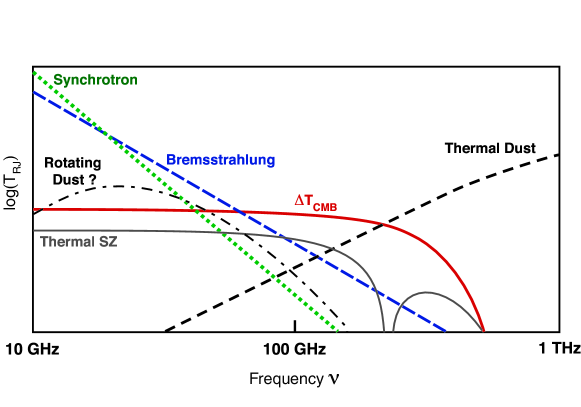
The separation of astrophysical components is possible essentially because the components have distinct emission spectra as a function of radiation wavelength. This is illustrated in figure 2. If the number of components and their respective spectra were perfectly well known, and if measurements were noiseless, then multifrequency observations (with at least as many observations as there are components) would allow in principle the recovery of the emission of each of the component at each point. Equation 1 still holds, but now indexes both time and detector number, and indexes both time and astrophysical component. The linear system can be large: the total number of measurements (i.e. the size of vector ) is , and the size of vector (the unknown) is . For Planck, the number of detectors is of the order of 100, the number of samples is of the order of a billion per timeline, the number of pixels of the sky is about one to 10 million, and the number of astrophysical processes is at least five or six (3 or 4 galactic components, CMB, and SZ - not mentioning complications arising for polarisation measurements).

This large system can not be handled by a brute force method. It can be simplified in some cases, if the noise is uncorrelated for instance. Assuming we dispose of clean maps of the sky at various frequencies, we can write:
| (7) |
where now indexes frequencies of observation, and indexes astrophysical components. is the mixing matrix, the value of the map at frequency in direction , and the emission of component . is the noise in measurement .
Equation 7 can be inverted by any of the standard methods as the COBE or the Wiener one mentioned in section 1. This can be done in real space (pixel by pixel), or in Fourier space (mode by mode), or on other basis of functions (wavelet by wavelet…), depending on the shape and the coverage of the maps, the geometry of the observations, and the correlation properties of the noise and the components.
For details about linear methods, we refer the reader to the papers by Tegmark [13] and Bouchet and Gispert [11], and for nonlinear methods to papers by Hobson et al. [5] and Baccigalupi et al. [6]. The Wiener method of Bouchet and Gispert has been extended recently to the separation of polarised components by Bouchet, Prunet and Sethi [14].
The trickiest part is getting the right model of the data : assuming the right number of components, knowing their spectra (matrix ) and knowing the properties of the noise. This is especially true as recent measurements seem to indicate the presence of microwave dust emission from rotating grains in addition to the usual thermal emission, for instance, which complicate even more the determination of the spectrum of the (always sub-dominant, or nearly so) free-free emission. Variations of the number of relevant components and of their statistical and spectral properties as a function of the region of the sky observed complicate the separation of components on full-sky maps. Clearly, although some efforts have been made recently in this direction, the separation of components by a Wiener method on full sky maps is in contradiction with the known properties of foregrounds (localised, position-dependent).
Future methods, probably, will have to take explicitely into account the effect of uncertainties in the model, including in the error estimates the impact of unknown errors in matrix .
5 Subtraction of slow drifts
Slow drifts are one of the lost fundamental problems we have to face for CMB anisotropy measurements. In most cases, this problem can be handled satisfactorily independently of the separation of astrophysical components. This decomposition of the problem of data reduction into subtasks with little loss in performance permits to handle very large data sets, as discussed by Bond and collaborators [10].
In the simplest model, slow drifts are simply due to noise. The total noise (including this low-frequency component) is stationnary, its spectrum is known, and the optimal reprojection of the data, taking into account the correlation of the noise, can be obtained in the COBE way, as discussed by Tegmark [4]. If the spectrum is not known, then one can estimate it from the data as in the method of Ferreira and Jaffe [8]. However, this last method relies on the assumption that the spectrum of the noise is somewhat smooth, as it is binned in ranges of frequencies. This is not necessarily the case (actually it is not the case in most of the examples I know) so the impact of this uncertainty in the model should be evaluated - and, if possible, taken into account for finding the best solution and errors.
Another method for slow drifts removal, which does not rely on prior knowledge of the noise spectrum, consists in modelling slow drifts as a function of a relatively small number of parameters , to be fitted as unknowns of the model. Formally, we write:
| (8) |
where is a function slowly varying with time, parametred by coefficients , modelling the effect of the slow drifts, and can now be assumed to be white. These coefficients, for instance, can be coefficient of the Fourier expansion of the timeline (or fractions of it) as in [9], or coefficients of splines used to fit the slow drifts. The system is then solved for and by minimising the :
| (9) |
An adaptation of this method in the context of the measurement of CMB polarisation has been implemented on simulated data by Revenu and collaborators [15].
In this method which seems to “fit the noise out”, the fact that the noise is essentially low-frequency comes in to allow the low frequency drifts to be modelled as a function of a small number of parameters, so that the total number of unknown is significantly smaller than the number of measurements. From Shannon sampling theorem, this is possible, for instance, if the knee frequency above which slow drifts become negligible is significantly smaller than the sampling frequency of the data. The slow drifts, then, can be “sampled” at a rate significantly slower than the sampling of the timeline, allowing for the number of parameters to be much less than the number of data points.
The method, clearly, requires a lot of redundancy in the data, as discussed in [16]. These redundancies should also be spread out along the timeline so that they allow sampling the slow drifts (using parameters ) at a sufficient rate.
6 The straylight problem
One of the most serious problem for most CMB anisotropy experiments, and especially for sensitive ones, is the problem of straylight. Minimising the total amount of unwanted radiation admitted into the detectors is a permanent instrumentalist’s nightmare. The correction of straylight effects in the data processing is a complicated problem, and is the object of active research. The first step is the estimation of the properties and levels of these effects for a mission such as Planck.
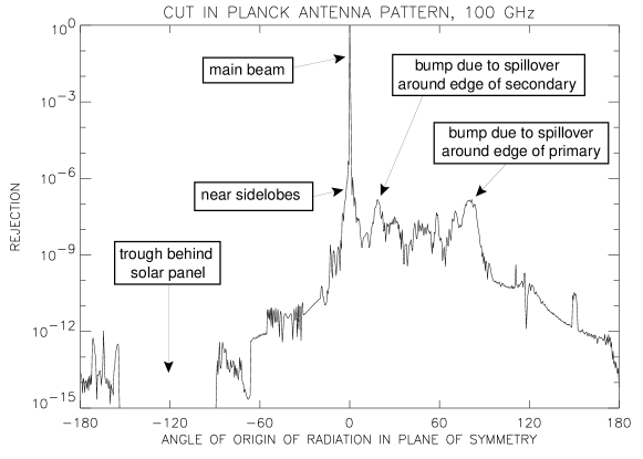
A model for the Planck antenna pattern has been computed at ESTEC by P. de Maagt and collaborators. Figure 3 displays a single cut of the antenna pattern (in the plane of symmetry of the satellite).

In terms of integrated emission as seen from solar neighborhood, the strongest sources of radiation in the submillimeter sky, relevant for the problem of straylight, are the Sun, the planets and the Moon, the galactic plane emission, and the CMB dipole.
The properties of the sidelobe pickup depend on the scan strategy. For Planck, the satellite is rotated around a spin axis offset by 85 degrees from the optical axis, so that the main beam corresponding to a given detector scans the sky along great circles about 85 degrees in diameter. The orientation of the spin axis is re-adjusted every hour or so to follow the apparent motion of the Sun in the sky, keeping the spin-axis roughly anti-solar. For details on the Planck scanning, see [17].
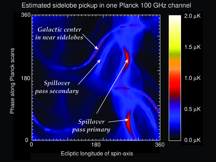
Using the Planck 100 GHz antenna pattern of P. de Maagt and a model of the sky featuring galactic emission scaled from the DIRBE 240m map and 408 MHz maps [18], we get estimated straylight signals due to the pickup of galactic emission in sidelobes for Planck. The result is displayed in figure 4. Although the total peak-to-peak straylight signal remains within reasonable limits (less than 2 K), its large-scale properties could generate spurious non-gaussianity at low , detectable by sensitive non-gaussianity tests. It is therefore a potential worry.

7 Conclusions
In this paper, I have reviewed the main issues and methods concerning the reduction of CMB data. I have emphasised on the importance of proper modelling for finding an optimal solution to this problem. The main issues for CMB data reduction are foregrounds (astrophysical or others), slow drifts of various origins in the timelines, and instrumental imperfections as the problem of straylight pickup in the detectors. Understanding the issues and the instrumental problems is important, as the optimisation of the reduction requires optimising the data model at least as much as optimising the numerical methods for solving the problem.
Standard linear methods for handling astrophysical foregrounds and slow drifts are now well established. These methods could still be improved by taking into account explicitely the uncertainty in the measurement model (lack of knowledge of the exact number of “sources” for component separation, imprecision in the knowledge of foreground spectra and statistical properties, imprecision in the knowledge of detector pointings).
Acknowledgements
Thanks to Jean-Christophe Hamilton and Alexandre Amblard for their critical reading of the original manuscript.
References
- [1] Hu, W. and Sugiyama, N.: Ap. J. 471, 542 (1996).
- [2] Jungman, G., Kamionkowski, M, Kosowsky, A. and Spergel, D.N.: Phys. Rev. D 54, 1332 (1996).
- [3] Wright, E.L., Hinshaw, G., Bennett, C.L.: Ap. J. 458, L53 (1996).
- [4] Tegmark, M.: Phys. Rev. D 56, 4514, (1997).
- [5] Hobson, M.P., et al.: MNRAS 300, 1 (1998).
- [6] Baccigalupi, C. et al.: preprint submitted to MNRAS, astro-ph/0002257 (2000).
- [7] Cayón, L. et al.: MNRAS 315, 757 (2000).
- [8] Ferreira, P.G. and Jaffe, A.H.: MNRAS 312, 89 (2000).
- [9] Delabrouille, J.: A&A Suppl. Ser. 127, 555, (1998).
- [10] Bond, J.R. et al.: Computing in Science and Engineering March-April 1999, 21 (1999).
- [11] Bouchet, F.R. and Gispert, R.: New Astronomy 4, 443 (1999).
- [12] Knox, L.: MNRAS 307, 977 (1998).
- [13] Tegmark, M.: Ap. J. 480, L87, (1997).
- [14] Bouchet, F.R., Prunet, S. and Sethi, Shiv K. : MNRAS 302, 663 (1999).
- [15] Revenu, B. et al.: A&A Suppl. Ser. 142, 499, (2000).
- [16] Delabrouille, J., Gispert, R., Puget, J.-L.: in “Fundamental parameters in Cosmology”, Proceedings of the XXXIIIrd Rencontres de Moriond, Editions Frontières (1998).
- [17] Delabrouille, J. et al.: Astro. Lett. and Communications 37, 259 (2000)
- [18] Haslam, C.G.T., Quigley, M.J.S. and Salter, C.J.: MNRAS 147, 405 (1970).