HST-NICMOS Observations of M31’s Metal Rich Globular Clusters and Their Surrounding Fields II. Results

Abstract

We have obtained HST-NICMOS observations of five of M31’s most metal rich globular clusters: G1, G170, G174, G177 & G280. For the two clusters farthest from the nucleus we statistically subtract the field population and estimate metallicities using $K$-$(J-K)$ color-magnitude diagrams (CMDs). Based on the slopes of their infrared giant branches we estimate [Fe/H] $=-1.22\pm 0.43$ for G1 and $-0.15\pm 0.37$ for G280. We combine our infrared observations of G1 with two epochs of optical HST-WFPC2 $V$-band data and identify at least one LPV based on color and variability. The location of G1’s giant branch in the $K$-$(V-K)$ CMD is very similar to that of M107, indicating a higher metallicity than our purely infrared CMD: [Fe/H]$\sim-0.9\pm 0.2$. For the three central clusters, which are too compact for accurate cluster star measurements, we present integrated cluster magnitudes and field CMDs.

The $K$-band luminosity functions (LFs) of the upper few magnitudes of G1 and G280, as well as for the fields surrounding all clusters, are indistinguishable from the LF measured in the bulge of our Galaxy. This indicates that these clusters are very similar to Galactic clusters, and at least in the surrounding fields observed, there are no significant populations of young luminous stars.

For the field surrounding G280, we estimate the metallicity to be $-1.3$ from the slope of the giant branch, with a spread of $\sigma_{[Fe/H]}\sim 0.5$ from the width of the giant branch. Based on the numbers and luminosities of the brightest giants, we conclude that only a small fraction of the stars in this field could be as young as 2 Gyr, while the majority have ages closer to 10 Gyr.

1 Introduction

Globular clusters (GC) occupy a very special position in modern astrophysics. They provide the most stringent tests of stellar evolution theory, represent ideal templates for stellar population synthesis studies, allow age dating of galaxies with unrivaled precision, etc. The GC families of the Milky Way and its satellite galaxies, the Magellanic Clouds and the Fornax dSph galaxy, have been thoroughly studied from both the ground and space, especially with HST. The next nearest major GC family belongs to M31. To study individual stars in GC systems much more distant than M31 will require the next generation of ground or space based telescopes.

The GC systems of the the Milky Way and M31 appear to be quite similar in luminosity and color ranges (Battistini et al., 1987; Elson & Walterbos, 1988; Huchra, Brodie & Kent, 1991; Frogel, Persson & Cohen, 1980b; Djorgovski et al., 1997; Seitzer, Banas & Armandroff, 1996). However, some of M31’s bulge globulars appear to have line strengths as strong as those of giant ellipticals, suggesting metallicities considerably greater than any known Galactic globular (Bica et al., 1992; Jablonka, Alloin & Bica, 1992; Jablonka, 1997). Burstein et al. (1984) has also noted that M31’s GCs appear to follow different H$\beta$ and CN correlations with Mg₂ with respect to Galactic globulars; they attributed this to the whole M31 GC family being systematically younger. Renzini (1986) pointed out that other interpretations were also possible, such as the chemical enrichment history of the two spheroids having proceeded with slightly different time scales, resulting in different element ratios.

HST observations of M31’s GCs in the optical (with the goal of stellar photometry) started soon after the first refurbishing mission, with both FOC and WFPC2 (Fusi Pecci et al., 1996; Rich et al., 1996; Ajhar et al., 1996), and now include some of the most metal rich clusters (Jablonka et al., 2000). The study of metal rich M31 globulars complements similar studies of Galactic bulge globulars within this still poorly known, yet crucial part of age-metallicity space. Near-IR observations are essential to study the brightest giants in an old, metal rich population, especially to determine bolometric luminosities. Metal rich globular and bulge giants, which are the brightest bolometrically and in the near-IR, are in contrast, many magnitudes fainter at optical wavelengths due to severe molecular blanketing. In extreme cases, $(V-K)$ can be as great as $\sim 10$ at the top of the AGB (Frogel & Whitford, 1987; Guarnieri et al., 1998) and these stars are likely to have escaped detection in M31 even with WFPC2.

Since the main sequences of the old populations in M31 are currently out of reach, one is forced to appeal to an alternative age indicator. Theory predicts that the highest luminosity reached on the AGB is a function of age (Iben & Renzini, 1983), a prediction extensively verified by observations of clusters in the Magellanic Clouds (Mould & Aaronson, 1986; Frogel, Mould & Blanco, 1990). In metal poor Galactic globulars, no stars are brighter than the theoretical RGB tip, as expected for a $\sim 14$ Gyr population. However, the AGB of more metal rich clusters ([Fe/H]$>-1$) extends $\sim 1$ magnitude above the RGB (Frogel, Persson & Cohen, 1983; Frogel & Elias, 1988; Guarnieri, Renzini & Ortolani, 1997), as it does in the Galactic bulge (Frogel & Whitford, 1987). For clusters, though, these bright stars are all LPVs. For both clusters and bulge population these luminous stars are now generally ascribed to high metallicity, rather than to young age (Frogel & Whitford, 1987; Guarnieri, Renzini & Ortolani, 1997). Hence, the presence of stars brighter than the RGB tip does not guarantee an intermediate age; consideration of their color, luminosity and frequency in the parent population is required before drawing conclusions about ages (Renzini, 1993).

In Cycle 7 we proposed to obtain NICMOS $JHK$ images of 5 metal rich globular clusters in M31. From these observations, we planned to achieve the following scientific goals: (1) explore the upper end of the GC luminosity function; (2) derive independent estimates for the metallicity of the M31 clusters and their adjacent fields from the slope and location of the NIR RGB (Kuchinski et al., 1995); (3) determine the frequency of luminous RGB and AGB stars (including LPVs) per unit luminosity; (4) compare the cluster results with observations of M31 field stars (5) compare the properties of the luminous stars in M31’s metal rich clusters to those in the Galactic bulge and Galactic globulars; (6) integrate these results with optical photometry and spectroscopy and explore implications for stellar evolution theory and the interpretation of the integrated light of distant galaxies.

One critical issue deserves special attention if any of these goals are to be attained: the effect of stellar crowding. We (Stephens et al., 2001, hereafter Paper I), have carefully analyzed the effects of blending on our NICMOS data. Through the creation of completely artificial clusters, we have calculated threshold- and critical-blending limits for each cluster and surrounding field. These limits determine the proximity to each cluster where reliable photometry can be obtained. These simulations allow us to quantify and correct for the effects of blending on the GB slope and width at different surface brightness levels.

This paper is organized as follows. Section 2 presents the reasons for selecting each cluster, and the details of the observations. Section 3 describes the reduction procedures, and gives a brief summary of the procedures and results on blending from Paper I. Section 4 presents the integrated photometry of the clusters, the CMDs and luminosity functions of the clusters and their surrounding fields, and metallicity estimates for G1, G280, and the G280 field. Our conclusions are summarized in Section 5.

2 Observations

We have obtained HST NICMOS images of five of M31’s metal rich globular clusters and their surrounding fields (Cycle 7; Program ID 7826). These observations are summarized in Table 1. Column (1) lists the ID of Sargent et al. (1977), columns (2) and (3) give the center of each field observed with HST, and column (4) lists the angular separation from the nucleus of M31. Columns (5-8) give previous metallicity estimates for each cluster based on: (5) absorption strengths from integrated optical spectra (Huchra, Brodie & Kent, 1991); (6) spectroscopy of metal lines (Jablonka, Alloin & Bica, 1992; Jablonka, 1997); (7) RGB morphology (Fusi Pecci et al., 1996; Rich et al., 1996; Jablonka, 1997); (8) integrated ground-based NIR colors (Frogel, Persson & Cohen, 1980b; Cohen & Matthews, 1994). The last column (9) gives the observation date of each target.

Table 1: M31 Globular cluster observations

ID	$\alpha$	$\delta$	r	[Fe/H]				Date
	(2000)	(2000)	(′)	HBK	JAB	F-P	NIR	UT
G001	00h32m47$\fs$2	39°$34^{\prime}48^{\prime\prime}$	152.3	-1.08	-0.52	-0.60(?)	-1.38	1998.07.18
G170	00h42m32$\fs$4	41°$10^{\prime}29^{\prime\prime}$	6.1	-0.31	0.20	high	$\cdots$	1998.08.10
G174	00h42m33$\fs$3	41°$17^{\prime}17^{\prime\prime}$	2.6	0.29	$>0.5$	$\cdots$	-0.13	1998.08.13
G177	00h42m34$\fs$4	41°$14^{\prime}04^{\prime\prime}$	3.2	-0.15	0.52	high	-0.32	1998.09.08
G280	00h44m29$\fs$5	41°$21^{\prime}36^{\prime\prime}$	20.5	-0.70	$\cdots$	-0.40(?)	-0.40	1998.09.13

G174 is the most metal rich cluster known in M31 (Huchra, Brodie & Kent, 1991; Jablonka, 1997). It and G177 have spectra with line strengths comparable to those of strong lined ellipticals, and stronger than the most metal rich Galactic globulars. G170’s lines are somewhat weaker, but still comparable to those of two of the most metal rich Galactic globulars, NGC6528 and NGC6553 (Barbuy et al., 1999; Cohen et al., 1999). G170, G174 and G177 are projected very close to the nucleus of M31. The G177 field, although not the closest to M31’s nucleus, lies along the major axis of M31 and has the highest number of detected stars, $\sim 7$ arcsec^-2, as well as the highest background, $\mu_{K}\sim 15.4$ magnitudes arcsecond^-2.

G280’s CMD has been characterized by Fusi Pecci et al. (1996) as similar to, but not quite as metal rich, as NGC6553, consistent with its near-IR colors (Frogel, Persson & Cohen, 1980b). In spite of G280’s similarity to G170, it lies much farther from the nucleus of M31, at a distance of $20.5^{\prime}$. G280 is also one of the most “open” clusters, making it one of the best clusters in our sample for individual stellar photometry.

Finally, G1 is the largest, brightest globular cluster in M31. This cluster is of particular interest because of its high metallicity despite its large distance ($152^{\prime}$) from the center of M31. Since it nearly fills a NIC2 frame, we also observed a nearby field to estimate the background stellar contribution. It turns out that G1 is far enough from M31’s center that field star contamination is negligible, and our control field yielded only 2 stars over the entire $20^{\prime\prime}$ dithered $K$-band field.

Our observations were taken with the NICMOS camera 2 (NIC2) which has a plate scale of $\sim$ 0$\farcs$0757 pixel^-1 and a field of view of 19$\farcs$4 on a side (376 arcsec²). The NICMOS focus was set at the compromise position 1-2, which optimizes the focus for simultaneous observations with cameras 1 and 2. All of our observations used the multiaccum mode (MacKenty et al., 1997) because of its optimization of the detector’s dynamic range and cosmic ray rejection. Observations with NIC1 will be described in a later paper concentrating on M31’s bulge.

Each of our targets was observed through three filters: F110W (0.8–1.4 µm), F160W (1.4–1.8 µm), and F222M (2.15–2.30 µm). These filters are close to the standard ground-based $J$, $H$, & $K$ filters. The observation of each cluster spanned three orbits of HST, with $\sim 42$ minutes of observing per orbit. This yielded total integration times of 1920s in F110W, 3328s in F160W, and 2304s in F222M (see Table 2).

We implemented a spiral dither pattern with 4 positions to compensate for imperfections in the infrared array. The dither steps were 0$\farcs$4 for the $J$ and $K$ band images, and 5$\farcs$0 for the $H$ band images. Thus the combined dithered images are $\sim 20^{\prime\prime}$ in $J$ and $K$, and $\sim 24^{\prime\prime}$ in $H$. We used the predefined sample sequences step32 with 22 samples in $J$ and 25 samples in $K$, and the step64 sequence with 21 samples in $H$.

We present $H$-band images of each cluster in Figures 1a-e. These images are the combination of 4 dither positions, and are $\sim 24^{\prime\prime}$ on a side. The $H$-band images are the deepest and also cover the most area as they were acquired using the largest dithers. Thus the $H$-band provides the deepest luminosity function, and gives us additional color information for LPV identification. The other analyses use primarily the $J$- and $K$-bands, as they are the bands where the groundbased comparisons, age-luminosity relations, and metallicity indicators exist.

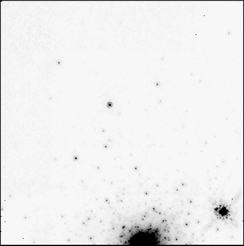
Figure 1: G1 – F160W ($H$-band) combination of all 4 dithers; 3328s total exposure. The faintest stars seen in this image have $H\sim 21.8$ magnitudes. The object in the lower right corner is a foreground star and gives an idea of the full NICMOS PSF.

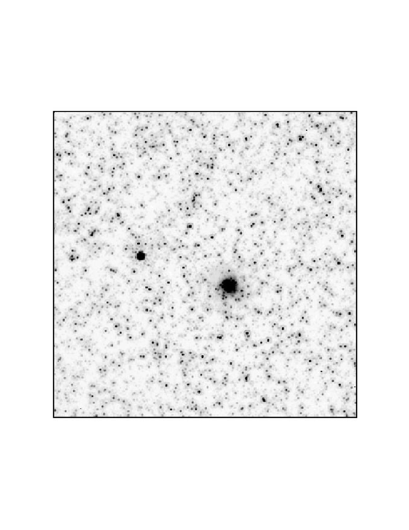
Figure 1b: G170 – Combination of 4 dithers in the F160W ($H$) filter, yielding 3328s total exposure time.

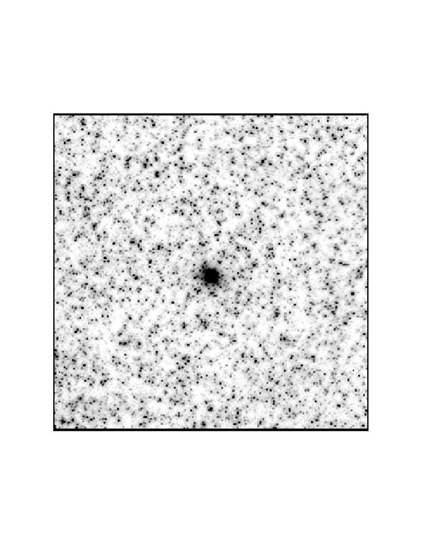
Figure 1c: G174 – same as Fig. 1b

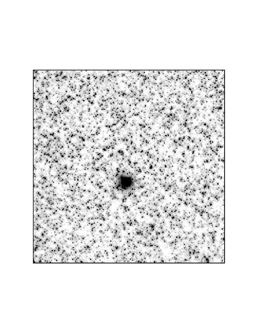
Figure 1d: G177 – same as Fig. 1b

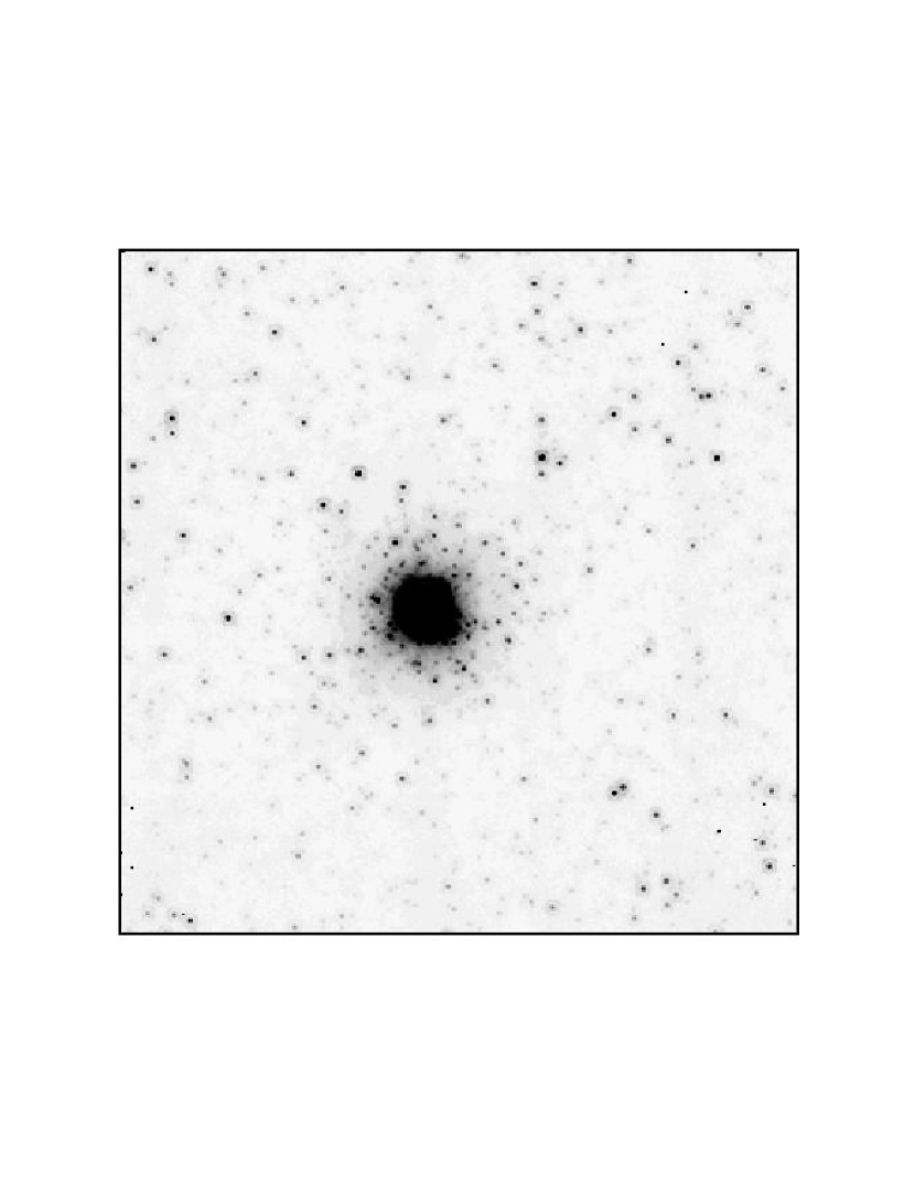
Figure 1e: G280 – same as Fig. 1b

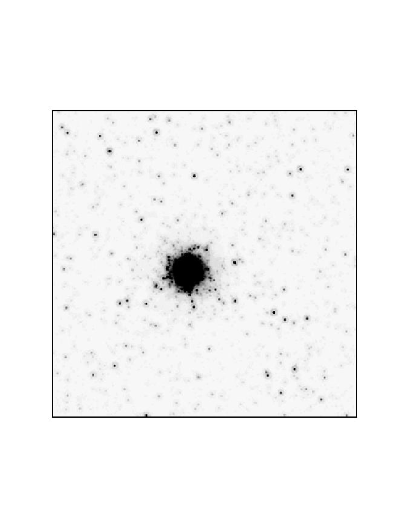
Figure 1f: A280 – The artificial analog of the G280 cluster and field. Note the similarity to the real frame displayed in Fig. 1e.

3 Data Reduction

Our data were reduced with the STScI pipeline supplemented by the IRAF NICPROTO package (May 1999) to eliminate any residual bias (the “pedestal” effect). Object detection was performed on a combined image made up of all the dithers of all the bands (12 images in total). PSFs were determined from each of the four dithers, then averaged together to create a single PSF for each band of each target (the average FWHM of each band is listed in Table 2). Instrumental magnitudes were measured using the ALLFRAME PSF fitting software package (Stetson, 1994), which simultaneously fits PSFs to all stars on all dithers. DAOGROW Stetson (1990) was used to determine the best magnitude in a $0.5^{\prime\prime}$ radius aperture, which we then converted to the CIT/CTIO system using the transformation equations of Stephens et al. (2000).

The azimuthally averaged number of detected stars per square arcsecond for each cluster is shown in Figure 7 as a function of radius from the cluster center. The counts include stars which were measured at least once in any band. Even though it appears we have detected stars into the centers of all the clusters, we have demonstrated in Paper I that the detections near the cluster cores are spurious, the result of image blending. The three clusters near the center of M31, G170, G174 and G177, have central spikes in the number counts, but quickly fade into the background. No photometry is possible for these clusters. For the two less compact clusters, G1 and G280, the number of detections decreases gradually with radius, and photometry is possible in their central regions.

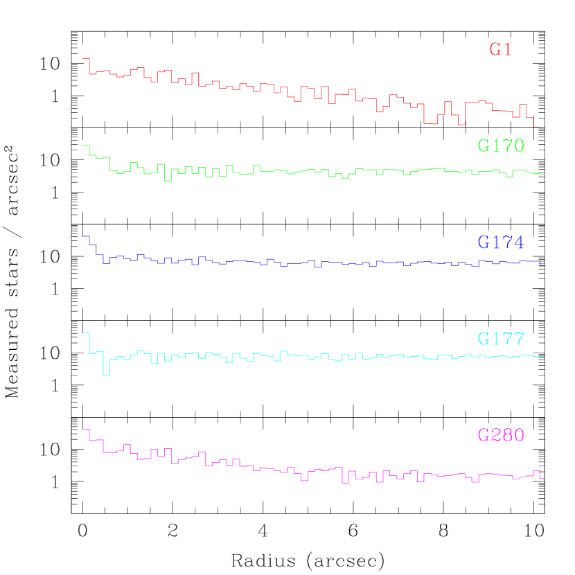
Figure 7: Number counts as a function of radius from the cluster center.

Table 2: NICMOS Filters

Filter	Exposure	FWHM
	(s)	(pix)	(′′)
F110W	1920	1.65	0.13
F160W	3328	1.95	0.15
F222M	2304	2.45	0.19

3.1 Blending Analysis

Stellar photometry in crowded regions such as we have observed can be strongly affected by blending. In order to quantify and attempt to correct for blending, we have performed several types of artificial star experiments; they are described in detail in Paper I. For these experiments we constructed completely artificial clusters. Starting with a blank frame having the appropriate noise characteristics, we added stars according to the cluster’s radial profile. The input stellar population was chosen to match the luminosity function and colors of giants observed in the Galactic bulge. The artificial frames were then processed and measured in exactly the same manner as the real data. As an example, A280, the artificial analog of the G280 cluster, is shown in Figure 1f. This frame is composed of 450,000 cluster stars and 80,000 field stars. The CMDs and LFs from the artificial clusters can be used to determine the origin of objects seen in the real CMD, and the validity of our measured LFs.

To better study the effects of blending at different surface brightness levels, we have also created uniformly populated mini-fields. Constructed in the same manner as the artificial clusters, these $100\times 100$ pixel fields each have between $10^{4}$ and $\sim 5\times 10^{6}$ stars, enough to reach the surface brightnesses observed in the cores of these M31 clusters.

Using Figure 9 of Paper I, which show the difference between the recovered and input stellar magnitudes as a function of the field surface brightness, we have chosen $\mu_{K}=16$ magnitudes arcsecond^-2 as the threshold surface brightness where our photometry starts to become noticeably affected by blending, and $\mu_{K}=14$ mag arcsec^-2 as the critical surface brightness where our photometry is dominated by blends, and no longer yields any useful information. Brighter than this level, no measurements are reliable. If one desires to accurately measure stars fainter than those we have measured, the threshold surface brightness will have to be fainter than $\mu_{K}=16$.

Figure 8 shows azimuthally averaged $K$-band surface brightness profiles of each cluster. Dotted lines indicate our chosen threshold- and critical-blending surface brightness levels. We use this plot to determine the threshold-blending radius ($R_{16}$), and the critical-blending radius ($R_{14}$) of each cluster. These radii are listed in Table 3. Any objects measured inside the threshold-blending radius, especially faint objects, are potentially affected by blending, and should be considered suspect. (Note that the radius $R_{16}$ was chosen so that stars input at $M_{K}\sim-3$ could be recovered accurately most of the time. However, for stars fainter than this, there is no way to tell whether stars measured at $M_{K}>-3$ are blends or not.) Objects measured inside the critical-blending radius are undoubtedly blends, and although we plot them for completeness, they should be disregarded.

Since we want to use the slope of the GB to estimate metallicities (Kuchinski & Frogel, 1995), and the width of the GB to place limits on any spread in metallicity, we have investigated the effects of crowding on these quantities. At low surface brightnesses ($\mu_{K}\sim 20$ magnitudes arcsecond^-2) blending has a negligible effect on the measurement of the GB slope, and the correct metallicity is calculated. As the surface brightness increases to $\mu_{K}\sim 13$ magnitudes arcsecond^-2, the recovered GB slope also increases (becomes more negative), yielding an artificially greater metallicity. Plotting the recovered GB slope as a function of surface brightness from the artificial frames, we have determined a linear correction to the slope in an attempt to account for the effects of blending (Fig. 11, Paper I); we apply this relation to our observed slope to improve our metallicity determinations. The true change in slope due to blending will, of course, depend upon the true luminosity function and stellar colors.

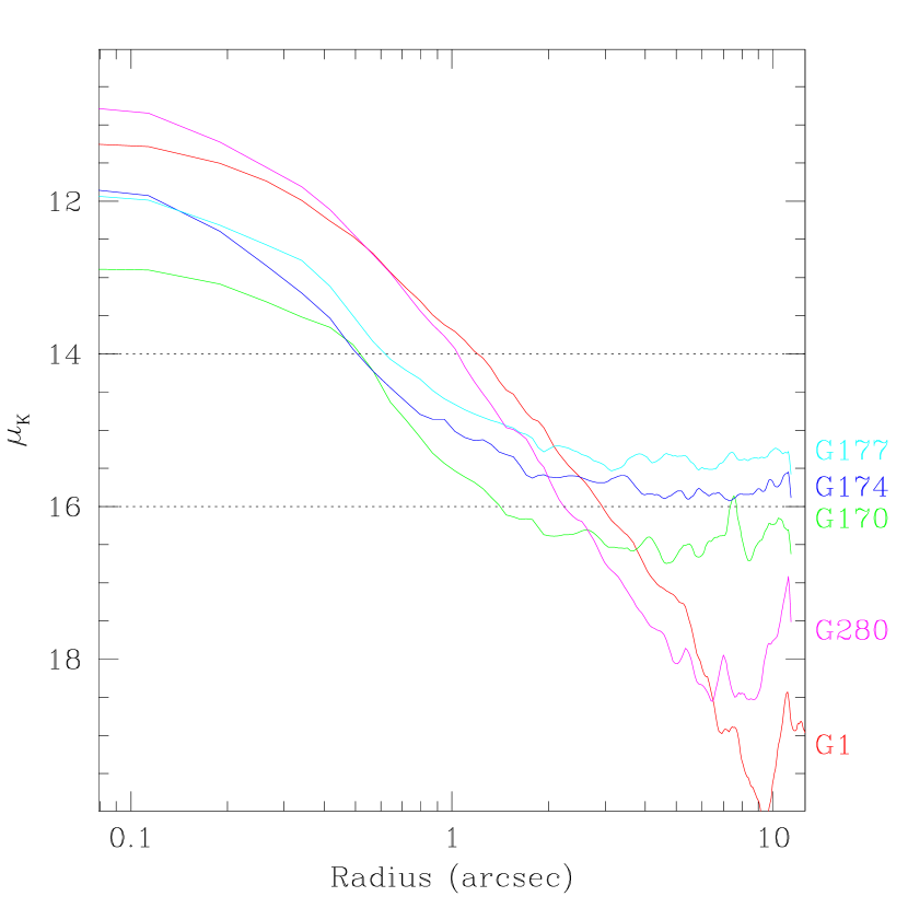
Figure 8: Azimuthally averaged $K$-band surface brightness as a function of radius from the cluster center.

Table 3: Threshold & Critical Blend Radii

Name	Core $\mu_{K}$	$R_{14}$	$R_{16}$
G001	11.2	1.2	2.9
G170	12.9	0.5	1.4
G174	11.7	0.5	$\cdots$
G177	11.8	0.6	$\cdots$
G280	10.7	1.0	2.2

4 Photometry

Here we present the integrated cluster photometry, and individual stellar photometry for the clusters and fields. Using the criteria developed in paper I, and summarized in §3.1 here, we reject measurements which may be affected by blending. As stated above, cluster star measurements could only be extracted for the two less compact clusters G1 and G280. For these two clusters we perform statistical subtraction of the field to yield a cluster GB. Our simple technique to do statistical subtraction divides the stars into cluster ($2.2<r<5^{\prime\prime}$) or field ($r>5^{\prime\prime}$), then partitions each into bins in $JK$ space, 1 magnitude wide in $J$ and $K$; we chose rather wide bins to allow for spread due to blending. The number of field stars per bin is then normalized by multiplying by the ratio of the cluster to field areas, and the appropriate number of suspected field stars are randomly subtracted from each of the cluster star bins. Using stars brighter than $M_{K}=-3.7$ and $M_{J}=-2$ and throwing away $3\sigma$ outliers, we perform an iterative linear least-squares fit to the GB. We then estimate the cluster metallicity using the GB slope technique (Kuchinski et al., 1995; Kuchinski & Frogel, 1995), and compare the M31 GBs with those measured for Galactic clusters. For the three central clusters, we present only the surrounding field photometry cleaned of any potential blends. The data are presented in the form of $M_{K}$-$(J-K)$ diagrams, as well as luminosity functions, and a $V$-$(V-K)$ diagram of G1 using optical WFPC2 data. All data assume $(m-M)=24.4$ and no reddening.

4.1 Integrated Photometry

Using simple aperture photometry, we have measured integrated magnitudes for G170, G174, G177, and G280 clusters. These measurements are listed in Table 4. The three central clusters (G170, G174 & G177) are very compact, and an aperture of 40 pixel ($3.03^{\prime\prime}$) radius is chosen as the optimum compromise between the maximum aperture size and best sky measurement. G280 is more extended, and we therefore use a 60 pixel ($4.54^{\prime\prime}$) radius aperture. The sky was measured as the average of an annulus around the clusters, using the largest outer radius possible, typically 60 pixels wide, stopping just short of the bright region at the bottom of all of the $K$-band frames. The formal errors are $J\pm 0.03$, $H\pm 0.03$, and $K\pm 0.04$, however, the measurements are very dependent on our sky level estimate. Since we are resolving, but trying to average out, the background stars, the sky estimate is sensitive to the size and location of the background region.

Previous measurements are listed on the right side of Table 4. Frogel, Persson & Cohen (1980b) used single-channel photometry with a $7.5^{\prime\prime}$ radius aperture. The Cohen & Matthews (1994) and Barmby et al. (2000) works used infrared arrays with $2.8^{\prime\prime}$ and $6^{\prime\prime}$ radius apertures respectively. Due to the limited size of our array, we were unable to match the large apertures of some of the previous measurements. However, our excellent resolution allows us to very carefully place our measurement aperture and sky annulus (e.g. to avoid the bright field star $\sim 7.4^{\prime\prime}$ from G170). The good color agreement but poor magnitude agreement with previous observations suggests a measurement problem that is present in all bands, and thus cancels out in the color determination. The most likely cause is the difference in the cluster and sky measurement regions between us and previous authors.

Table 4: Integrated Photometry

	NICMOS				Ground-based
Cluster	$K$	$J-K$	$H-K$	ap	$K$	$J-K$	$H-K$	ap
G170	12.93	0.98	0.36	3.0	12.84	0.98	$\cdots$	6.0
G174	12.56	1.03	0.47	3.0	12.84	1.00	$\cdots$	2.8
G177	12.36	0.98	0.39	3.0	12.50	0.92	$\cdots$	2.8
G280	10.91	0.89	0.33	4.5	11.06	0.88	0.15	7.5

Table 5: G1 & G280 Metallicities

Reference	G1	G280
Harris & Canterna (1977)	$-0.3$	$0.0$
Frogel, Persson & Cohen (1980b)	$-1.22$	$-0.19$
Bònoli et al. (1987)	$-1.23$	$-0.37$
Heasley et al. (1988)	$-0.7$	$\cdots$
Huchra, Brodie & Kent (1991)	$-1.08$	$-0.70$
Jablonka, Alloin & Bica (1992)	$-0.52$	$\cdots$
Rich et al. (1996)	$-0.8$	$\cdots$
Fusi Pecci et al. (1996)	$-1.14$	$-0.44$
This work: $(J-K)$ CMD	$-1.22\pm 0.43$	$-0.15\pm 0.37$
This work: $(V-K)$ CMD	$-0.9\pm 0.2$	$\cdots$

4.2 G1

The $M_{K}$-$(J-K)$ color magnitude diagram for the G1 cluster is shown in Figure 9. The left panel shows all the cluster data from the G1 frame. Open circles indicate objects which are located inside the threshold-blending radius ($2.9^{\prime\prime}$), or lie in a region of high background in the lower 25 pixels of the the $K$-band frames (on the CMD, these stars include all objects with $(J-K)>1.6$, and a similar number of objects bluer and fainter). Objects inside the critical-blending radius ($1.2^{\prime\prime}$) are plotted with half-size dots. The center panel shows the (two) objects measured in the adjacent control field located $64^{\prime\prime}$ SE of G1. The right panel shows only good measurements of cluster stars. Potentially blended objects and objects within 25 pixels of the bottom of the frame have been removed, and (two) field stars have been statistically subtracted.

We applied a linear least-squares fit to the cluster stars on the upper GB, only using stars brighter than $M_{K}=-3.7$ and $M_{J}=-2$, the 50% completeness limits, and ignoring $3\sigma$ outliers. The best-fit equation is displayed at the top of the right panel. We then used the relationship between the GB slope and globular cluster metallicity derived by Kuchinski et al. (1995); Kuchinski & Frogel (1995) for Galactic globulars to estimate the cluster metallicity. This relation states that [Fe/H]$=-2.98-23.84\times slope_{GB}$. Our measured GB slope is $-0.083\pm 0.014$, which implies a metallicity of $-1.00\pm 0.42$. The error estimate is a quadratic combination of the error in our linear fit, and the quoted 0.25 dex scatter observed in the GB slope – metallicity relation. Note that the range in our fitted $M_{K}$ (3 mags) is significantly smaller than the range (4.5 mags) Kuchinski & Frogel (1995) used to define the relation.

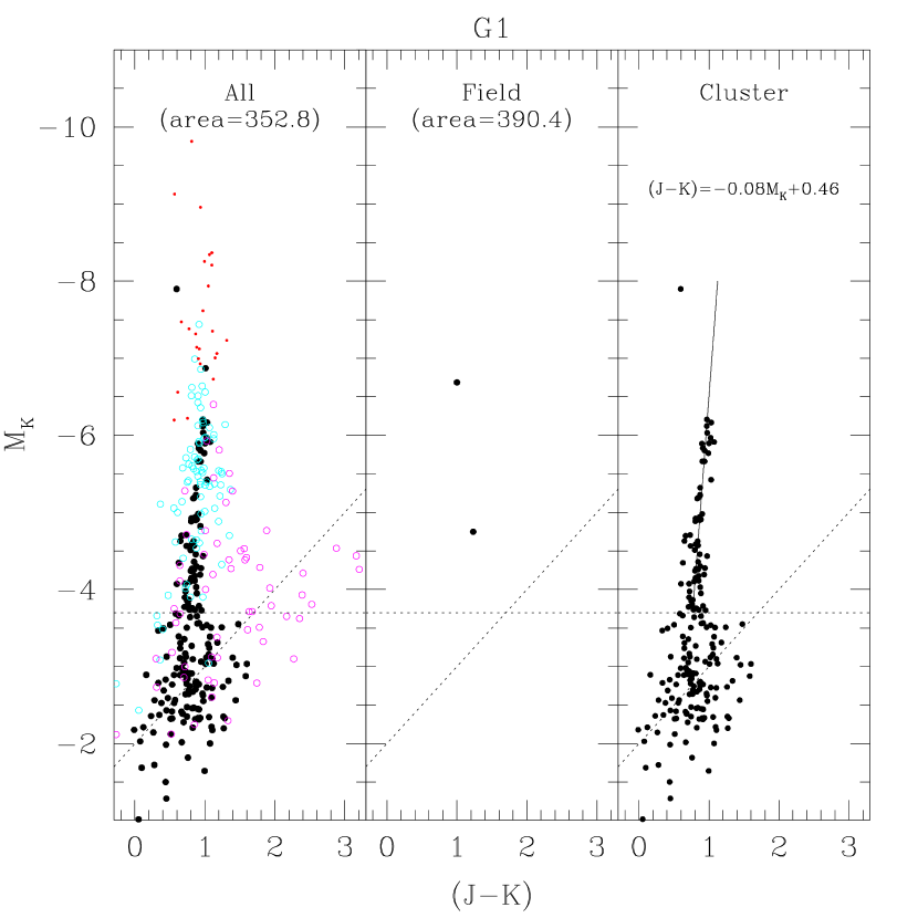
Figure 9: G1 – Left: All objects measured on the G1 frame. Open circles indicate objects within the threshold-blending limit ($\mu_{K}<16,r<2.9^{\prime\prime}$) or within 25 pixels of the bottom of the $K$-band image. Half-size dots are for objects inside the critical-blending limit ($\mu_{K}<14,r<1.2^{\prime\prime}$). Center: Stars measured in the adjacent control field $64^{\prime\prime}$ SE of G1. Right: Cluster stars remaining after potential blends, noisy measurements, and field stars have been removed. The linear fit to the GB above the 50% completeness limits of $M_{K}=-3.7$ and $M_{J}=-2$ (dashed lines) is shown at the top.

As discussed in §3.1, the measured slope of the GB is affected by blending, even at relatively low surface brightnesses. Ideally we would calculate the GB slope in several annuli, and correct each according the the average SB in that annulus. In reality, there are so few stars that are measurable on the upper GB to begin with, that splitting it up into even two annuli degrades the accuracy of the slope determination significantly. Thus we take a number – weighted average surface brightness of $\mu_{K}=18.4$ for all usable cluster photometry, which leads to a metallicity correction of $-0.22\pm 0.09$ dex, where the error of 0.09 dex is the rms scatter around our correction. This gives a final metallicity estimate of $-1.22\pm 0.43$ for G1.

We have combined our infrared NICMOS data with the $V$-band WFPC2 observations of Rich et al. (1996) (1994.07.29) and Meylan et al. (2000) (1995.10.02). The resulting $K$-$(V-K)$ CMD is shown in Figure 10. In this diagram, the points indicate the mean $(V-K)$ obtained from both optical datasets. The errrorbars illustrate the range of the observed $V$-band measurements. Since the measurement errors are relatively small, any large deviations are assumed to be indicative of stellar variability. Thus several of the most luminous stars near the top of the GB are undoubtedly variables. We have also over-plotted the RGB ridge lines of M13 and 47 Tucanae from Frogel, Persson & Cohen (1981), and stars in M107 from Frogel, Persson & Cohen (1983). We point out that the G1 RGB appears to lie blue-ward of 47 Tuc, and nearly on top of the M107 measurements. This indicates that G1 probably has a slightly higher metallicity ([Fe/H]$\sim-0.9$) than we obtained from the slope of the infrared GB.

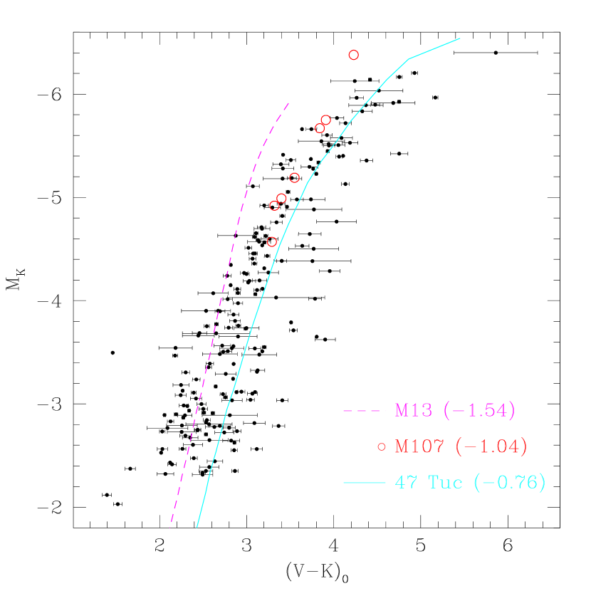
Figure 10: G1 CMD created through the combination of our $K$-band data with the WFPC2 $V$-band observations of Rich et al. (1996) and Meylan et al. (2000). The points are the mean $(V-K)$ from both optical datasets, and the errorbars illustrate the difference between the two optical datasets. Thus large errorbars indicate variability at the top of the CMD, and most likely misidentifications at the bottom of the CMD. G1 has been corrected for distance and reddening with $(m-M)=24.4$ and $E(V-K)=0.28$ (Frogel, Persson & Cohen, 1980b). Over-plotted are the giant branch ridge lines of M13 (dashed line) and 47 Tuc (solid line) from Frogel, Persson & Cohen (1981). Measurements of single stars in M107 from Frogel, Persson & Cohen (1983) have also been plotted for reference. The metallicities (in parentheses), distances and reddening for each cluster were taken from Harris (1996).

Previous measurements of G1’s metallicity are listed in Table 5. Harris & Canterna (1977) used Washington photometry of the integrated light to obtain a value of -0.3. Frogel, Persson & Cohen (1980b) used the integrated $(V-K)$ colors and the infrared CO index, finding [Fe/H]$=-1.22$. Bònoli et al. (1987) recalibrated the Frogel results using the new [Fe/H] values of Zinn & West (1984), obtaining [Fe/H]$=-1.23$. Based on the GB position in the $I$-$(V-I)$ diagram, Heasley et al. (1988) estimated a metallicity of $\sim-0.7$, and Rich et al. (1996) found a metallicity “at least as high as 47 Tuc”. Using the strengths of absorption features in integrated optical spectra, Huchra, Brodie & Kent (1991) found a metallicity of $-1.08$. Averaging the metallicities from many metallic lines in the spectral range $\lambda\lambda 3200-9750$Å, Jablonka, Alloin & Bica (1992) determined $\log(Z/Z_{0})=-0.52$ Most recently, Fusi Pecci et al. (1996) using the $(V-K)_{0}$ color, and the calibration from Brodie & Huchra (1990) found [Fe/H]$=-1.14$.

Our two metallicity determinations for G1 are different, but not inconsistent. We note that the value from the $(J-K)$ CMD ([Fe/H]$=-1.22\pm 0.43$) is based on a very small luminosity range, and has quite large errors. The estimate from the appearance of the $(V-K)$ CMD ([Fe/H]$\sim-0.9$) is less quantitative, but probably more robust.

There have been suggestions that the stars in G1 may have a range in metallicity (Jablonka et al., 1999), possibly due to self-enrichment. If this is so, we should be able to detect a spread in color in our near-IR CMDs. However, we find no evidence for such a spread as the dispersion in either the $(J-H)$ or $(J-K)$ colors: $\sigma_{(J-H)}=0.06$ in the range $-3>M_{H}>-6$, and $\sigma_{(J-K)}=0.04$ in the range $-4.5>M_{K}>-6.5$. These are both very close to the spread expected solely from measurement errors, as predicted by the artificial cluster A1, and by the ALLFRAME photometric uncertainties.

4.3 G280

The G280 $M_{K}$-$(J-K)$ CMDs are shown in Figure 11. The left panel shows all the data inside a radius of $5^{\prime\prime}$, the radius chosen to define the cluster. Objects inside the threshold-blending limit ($\mu_{K}<16$, $r<2.2^{\prime\prime}$) are plotted with open circles, and objects inside the critical-blending limit ($\mu_{K}<14$, $r<1.0^{\prime\prime}$) are plotted with half-size dots. The center panel shows all objects outside the $5^{\prime\prime}$ cluster radius. These stars are expected to be non-cluster, or “field” stars. The right panel shows the result of statistically subtracting the field star component from the cluster. We also omit any objects we suspect may be affected by blending, so that only objects in the annulus between the threshold-blending radius $(2.2^{\prime\prime})$ and the cluster radius $(5^{\prime\prime})$ are included.

We apply a linear least-squares fit to the cluster stars brighter than $M_{K}=-3.7$ and $M_{J}=-2$, ignoring $3\sigma$ outliers. The best-fit equation is displayed at the top of the right panel. Using this slope $(-0.136\pm 0.011)$ and the GB slope – [Fe/H] relationship of Kuchinski & Frogel (1995) we estimate the metallicity of the G280 cluster as $+0.26\pm 0.36$.

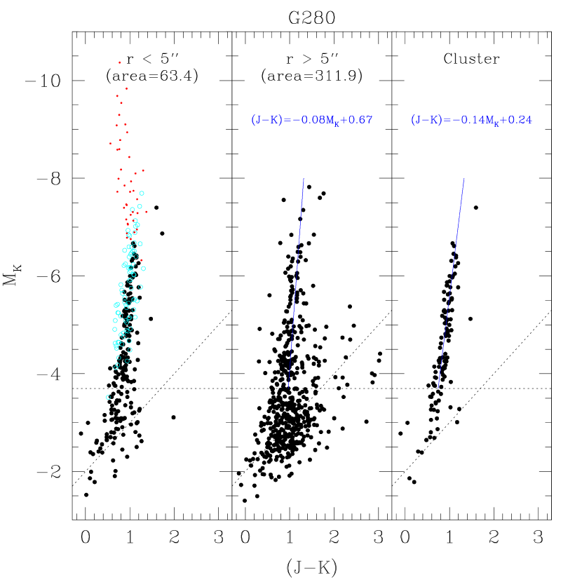
Figure 11: G280 – Left: all objects measured within $5^{\prime\prime}$ of the cluster center. Open circles indicate objects within the threshold-blending limit ($\mu_{K}<16$, $r<2.2^{\prime\prime}$), and half-size dots are for objects inside the critical-blending radius ($\mu_{K}<14$, $r<1.0^{\prime\prime}$). Center: objects farther than $5^{\prime\prime}$ from the cluster. Right: statistically field subtracted cluster GB and the linear fit. The dashed lines at $M_{K}=-3.7$ and $M_{J}=-2$ indicate the 50% completeness limits, and all fits disregard data fainter than these limits.

Again, as mentioned in §3.1, the measured slope, and thus the calculated metallicity, will be affected by blending. As in the case of G1, there are so few stars on the upper GB, that splitting it up into annuli significantly degrades the accuracy of the slope determination. We thus take a number – weighted average surface brightness of $\mu_{K}=16.9$ for the G280 cluster. This indicates a metallicity correction of $-0.42\pm 0.09$ dex is required to remove the effects of blending. Applying this correction gives a final metallicity of $-0.15\pm 0.37$ for the G280 cluster.

Previous metallicity measurements for G280 are listed in Table 5, and the techniques were briefly discussed in §4.2. These measurements cover a fairly large range, but our value is consistent with most.

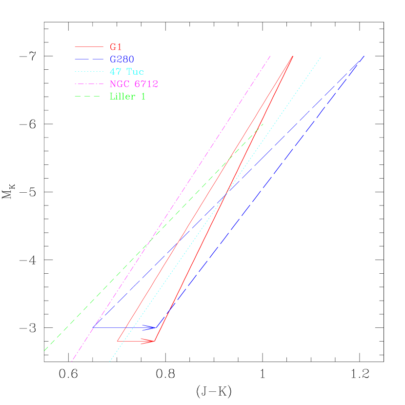
Figure 12: Linear fits to the G1 and G280 giant branches. The arrows show the shifts estimated for the blending corrections. Also shown are the GB fits and metallicities of the Galactic globular clusters 47 Tucanae [Fe/H]=-0.76, NGC 6712 [Fe/H]$=-1.01$, and Liller 1 [Fe/H]$=-0.2$.

We also looked for a possible intrinsic color spread, and hence a metallicity spread in G280. Such a metallicity spread would not be too surprising, since G280 is also a very massive cluster, with a velocity dispersion which is actually higher than that of G1 (Djorgovski et al., 1997). However, the dispersion in the measured colors is small, $\sigma_{(J-H)}=0.07$ $(-3>M_{H}>-6)$, $\sigma_{(J-K)}=0.08$ $(-4.5>M_{K}>-6.5)$, close to the spread expected solely from measurement errors. Thus we conclude that, as for G1, G280 does not show any significant metallicity spread.

Figure 12 shows the linear fits to the G1 and G280 giant branches before and after the blending correction. Also shown are three Galactic globular clusters which cover a range in metallicities. This figure gives an idea of the relative positions of G1 and G280 in CMD space, as well as the magnitude and direction of the blending corrections applied to the GB slopes.

The luminosity functions of the G1 (short-dashed) and G280 (long-dashed) clusters are shown in Figure 13. They both appear to have a sharp cutoff at $M_{K}\sim-6.5$, which is consistent with what is observed in Galactic globulars (Ferraro et al., 2000). We also show the Galactic bulge LF measured by Frogel & Whitford (1987) in Baade’s Window (solid) which has a sharp cutoff at $M_{K}\sim-7.5$. The faint end of G280 drops off more quickly than that of G1 since it is closer to the nucleus of M31 and the background is higher, making it more difficult to detect fainter stars.

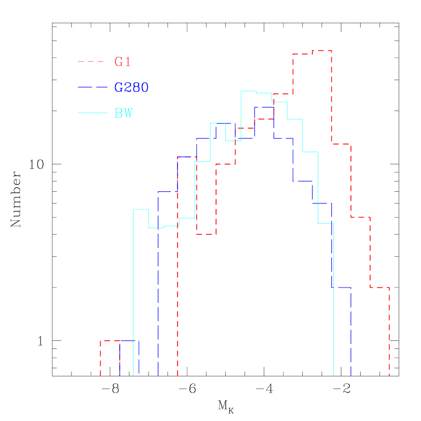
Figure 13: The G1 and G280 cluster luminosity functions. Also shown is the scaled Baade’s Window LF from Frogel & Whitford (1987).

4.4 Central Clusters

The three central clusters (G170, G174, & G177) are so compact that we were unable to extract any photometry of the cluster stars themselves. The star counts seem to indicate that the clusters were detected, but the detections occur in the regime where the effects of blending are considerable. Thus for these three clusters we present only the calibrated field CMDs in Figure 14.

We use the same blending criteria as the other clusters, developed in Paper I. Objects inside the critical-blending limit $(\mu_{K}=14)$ are plotted with half-size dots, and should be ignored. (see Table 3 for the specific radii of each cluster). These are the brightest and bluest stars on the upper RGB of each cluster. Objects located inside the threshold-blending limit $(\mu_{K}=16)$ are plotted with open circles, and should be considered dubious, note that nearly all the stars in the G174 and G177 clusters are such dubious measurements. We provide a linear fit to the GB measured in the G170 field, but do not attempt to estimate a metallicity, as the effects of blending are greater than we feel comfortable trying to correct.

As is evident from the radial surface brightness plots in Figure 8, the stellar density of these central fields is exceedingly high. G174 is the closest to the the nucleus of M31, and G177 is only slightly farther away, but lies along M31’s major axis. The surface brightness of these two clusters never drops below the threshold blending limit. We are therefore skeptical of this photometry, and do not provide GB fits. The artificial cluster A177 (the analog of G177), revealed brightening even in the field of up to 0.6 magnitudes at $K$ due to blending.

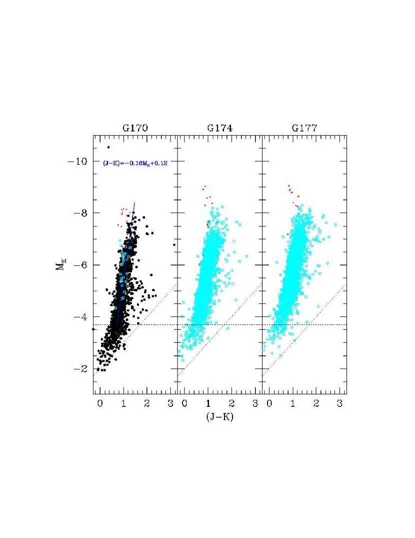
Figure 14: CMDs of the fields around G170, G174, and G177. We provide a linear fit to the GB of the G170 field, where the crowding is not too severe. This fit ignores points inside the critical-blending radius (half-size dots), points inside the threshold-blending radius (open circles), and objects fainter than $M_{K}=-3.7$ or $M_{J}=-2$.

4.5 Surrounding Fields

Figure 15 shows the scaled luminosity functions for the fields surrounding the cluster observations. The G1 field is not included as it is assumed that almost all of the stars are cluster members since only 2 were found in the nearby control field. The G280 field includes all stars that are greater than $5^{\prime\prime}$ from the cluster center. For the central clusters, we plot everything outside their threshold-blending radii, which are listed in Table 3.

All the field LFs look approximately the same, allowing for differences in the faint end due to varying levels of incompleteness. They all have an upper limit of $M_{K}\sim-8$, similar to what has been measured in the Galactic bulge where Frogel & Whitford (1987) observed a sharp break at $M_{K}\sim-7.5$ and stars trailing off to $M_{K}\sim-8.5$. These observations imply that the bulge of M31 has a stellar population not significantly younger than that in Baade’s Window, contrary to some previous observations. We will address this issue in more detail when we present our NICMOS data targeted at M31’s bulge

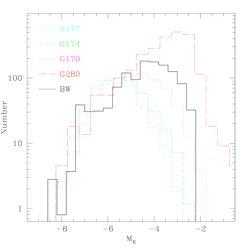
Figure 15: Normalized luminosity functions for the fields around each cluster, and the Baade’s Window LF from Frogel & Whitford (1987). The similarity of these LFs to the BW LF indicates that there is no significant population of bright young stars in the bulge of M31.

4.5.1 The G280 Field

Of all the field observations, the G280 field is the least crowded, and the only one where we feel comfortable performing a giant branch analysis. The field CMD is shown in the center panel of Figure 11. The linear fit to the GB, rejecting points fainter than $M_{K}=-3.7$ and $M_{J}=-2$, as well as $>3\sigma$ deviants, is shown at the top of the panel. The slope of the GB is $-0.081\pm 0.022$, which yields a metallicity of $-1.05\pm 0.58$ from the relation of Kuchinski & Frogel (1995). The average surface brightness of the field is $\mu_{K}\sim 18.3$, which requires a metallicity correction of $-0.23\pm 0.09$ dex to compensate for the effects of blending (see §3.1). Thus our final estimate of the metallicity of the G280 field is $-1.28\pm 0.59$.

The large error associated with the field metallicity estimate is not due to measurement errors, but rather to the very large spread in color. The dispersion in the $(J-H)$ color is $\sigma_{(J-H)}\sim 0.10$, and the dispersion in the $(J-K)$ color is $\sigma_{(J-K)}\sim 0.14$, both of which are significantly larger than the measurement errors. This spread in color is most likely due to a true spread in metallicity. Such a spread is not unexpected, since this field samples both the disk and bulge populations.

Frogel, Cohen & Persson (1983) have empirically determined a relationship between the GB $(J-K)$ color at $M_{K}=-5.5$ and the cluster metallicity using 12 Galactic globulars with [Fe/H] $<-0.8$. This relation has been recently revised by Ferraro et al. (2000) using 10 GGCs with more accurate distances: [Fe/H] $=4.76\times(J-K)_{0}(GB)_{-5.5}-5.38$. The measured spread in $(J-K)$ for the M31-G280 field is $\sigma_{(J-K)}\sim 0.14$ in the range $-4.5>M_{K}>-6.5$. We estimate the $(J-K)$ spread due to measurement errors as $\sigma_{(J-K)}\sim 0.04$ (also the spread measured in G1). Thus the intrinsic spread in color is $\sigma_{(J-K)}\sim 0.13$. Using the Ferraro et al. (2000) relation, this leads to a spread in metallicity of $\sigma_{\rm[Fe/H]}\sim 0.6$,

Since our $J$ and $H$ band data are the deepest, we have used the evolutionary tracks of Girardi et al. (2000) to derive a relation between the GB $(J-H)$ color at $M_{H}=-4$ and the cluster metallicity. We find that: [Fe/H] $=4.76\times(J-H)_{0}(GB)_{-4.0}-4.27$. In the G280 field the measured spread in $(J-H)$ is $\sigma_{(J-H)}\sim 0.10$ in the range $-3.0>M_{H}>-6.0$. We estimate the spread in $(J-H)$ due to measurement errors is $\sigma_{(J-H)}\sim 0.06$ (also the spread measured in G1). Thus the intrinsic spread in $(J-H)$ color is $\sigma_{(J-H)}\sim 0.08$. Using our relation derived from the evolutionary tracks, this corresponds to a spread in metallicity of $\sigma_{\rm[Fe/H]}\sim 0.4$,

Combining these measurements, keeping in mind that the $(J-H)$ data have higher signal-to-noise, and the $(J-K)$ relation is empirically determined, we estimate that the true spread in metallicity for the G280 field is $\sigma_{\rm[Fe/H]}\sim 0.5$. Note that no correction for blending is required, since our analysis shows no significant blending effects until brighter than $\mu_{K}\sim 16$ magnitudes arcsecond^-2

4.5.2 M31’s Disk

One would expect, that at $20.5^{\prime}$ from the center of M31, the field surrounding G280 should have a significant contribution from M31’s disk. However, the luminosity function of this field looks very similar to those obtained in our fields in the bulge of M31. In this section, we estimate the disk contribution to this field, and an age for this disk component based on the luminosity of the brightest AGB stars.

To find the relative contributions of the disk and bulge, we use the bulge–disk decomposition of Kent (1989). We take the position of G280 as $20.5^{\prime}$ from the center of M31, and 34° from the major axis. An interpolation of Kent’s data shows that G280’s position corresponds to a major axis distance of $\sim 23.8^{\prime}$, where the $r$-band surface brightness is $\mu_{r}=21.23$ magnitudes arcsecond^-2. The decomposition reveals that 85% of the flux is from the disk ($\mu_{r}(disk)=21.4$), and 15% is from the bulge ($\mu_{r}(bulge)=23.3$). Thus the stellar population of the disk should be well represented in the G280 field.

To estimate the age of the disk stars in our field, we first convert our $K$-band measurements to bolometric luminosities using the corrections of Frogel, Persson & Cohen (1980a). These corrections use the $(J-K)$ color, and we apply their M-star correction since this is a relatively high metallicity field. The results show that the brightest stars are mostly fainter than $M_{bol}\sim-5$.

Assuming that these few bright stars are members of a young population, we can estimate the age of this population using the relationship between AGB tip luminosity and age. First used by Mould & Aaronson (1979, 1980), this relation makes use of the monotonically decreasing maximum luminosity of the TAGB with age. Theoretically this relation is valid only for populations which are homogeneous in age and chemical composition, certainly not what we are observing in this field. However, as we will show, the dependence with metallicity is small (see Fig 16), and we are only trying to estimate the age of the youngest stars from the brightest observed $M_{bol}$. Due to the limited number of stars in our field, and the short lifetime at the TAGB, this estimate is only an upper limit to the age of the youngest stars.

We have calculated this relation using the ZVAR synthetic CMD code of Bertelli et al. (1992) (see also Gallart et al., 1996, 1999, for descriptions) to produce a synthetic CMD with constant SFR from 15 Gyr to 7 Myr ago, and metallicity increasing linearly with time using the Bertelli et al. (1992) stellar evolution models. We have used the mass-loss prescription of Vassiliadis & Wood (1993), (see Gallart et al. (1996) for a discussion on the effects of different mass loss prescriptions on the AGB morphology of CMDs of composite stellar populations). Of all the parameters used, mass loss is the one that has the strongest effect on the magnitude of the TAGB as a function of age.

This relation differs from that derived by (Mould & Aaronson, 1982) in which they use a mass loss treatment as parameterized by Reimers (1975) with $\eta=0.45$. At any given age, our predicted TAGB is $\sim 0.5$ mag fainter (Fig 16), and as a consequence we are deriving younger ages for stars of the same apparent magnitude.

Figure 16 illustrates our results for several different scenarios. As previously stated, all cases use constant SFR from 15 Gyr to 7 Myr ago, metallicity increasing linearly with time and the Bertelli et al. (1992) stellar evolution models. The first three lines listed in the legend all use the newer mass loss prescription of Vassiliadis & Wood (1993), and show the relative insensitivity of the TAGB luminosity to binary fraction and metallicity. The first model (long dash) has Z increasing from 0.0003 to 0.003 with no binaries. The second model (short dash) has the same metallicity, but now with 25% binaries. The third (short/long dash) has Z increasing from 0.002 to 0.01 with no binaries. We fit these three models with a smooth polynomial and plot it with a solid line. It is this fitted relation ($m_{bol}(TAGB)=-401.42+126.16\log(age)-13.492\log(age)^{2}+0.48499\log(age)^{3}$) which we use to estimate the age of the youngest stars in the G280 field. For comparison we show the luminosity – age relation of Mould & Aaronson (1982) which uses mass loss from Reimers (1975). We have also run our low-metallicity, no binaries model using the Reimers mass loss prescription, and it falls on the Mould & Aaronson (1982) relation. This verifies that the primary difference is indeed the treatment of mass-loss.

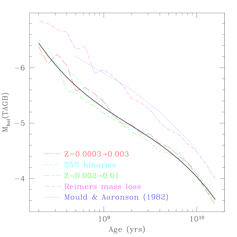
Figure 16: Theoretical luminosity of the AGB tip as a function of population age. Our calculations use constant star formation from 15 Gyr to 7 Myr ago, metallicity increasing linearly with time, and the Bertelli et al. (1992) stellar evolution models. The solid line is a polynomial fit to the three models using the Vassiliadis & Wood (1993) mass loss prescription.

Using the relation just developed, we estimate the age of the youngest stars in the G280 field. Considering only the single measurement of the bolometric luminosity of the brightest star in our field of $M_{bol,m}=-5.0$, we estimate an age of $\sim 2$ Gyr. One can also attempt to statistically estimate the tip of the AGB using the technique of Aaronson & Mould (1982). In this case one averages the stellar luminosities brighter than $-4.5$, and assuming that the distribution of stars along the AGB is uniform, the peak luminosity is twice the mean. Following this procedure, we average the (two) stars brighter than $-4.5$ and find a mean of $\overline{M_{bol}(<-4.5)}=-4.8$. which leads to an AGB tip luminosity of $M_{bol,f}=-5.15\pm 0.28$ for a fully populated AGB. According to our relation derived from the stellar models, this implies an age of $1.3^{+1.1}_{-0.6}$ Gyr for the disk stars in this field. Thus we conclude that the youngest component of this field can be as young as 1-2 Gyr based on the luminosities of the brightest giants.

Although the measured GB color of the G280 field is very similar to that of Baade’s Window, it is not inconsistent with having a small component of the population as young as 2 Gyr. This is because the GB color is not very sensitive to age. Our models show that at $M_{K}=-6$ the $(J-K)$ color only changes by $\sim-0.05$ going from 10Gyr to 2Gyr. This is confirmed by the Yale Isochrones using the LeJeune color tables to get infrared colors.

5 Conclusions

We first present surface brightness profiles of all clusters, and with the blending analysis presented in Paper I, determine radial photometric limits for each cluster. We then give integrated photometry of all clusters except G1, which was not fully on the detector.

For the G1 cluster, we present the infrared CMD, and estimate the metallicity as [Fe/H]$=-1.22\pm 0.43$ from the slope of the giant branch. Based on the width of the giant branch, which shows no significant spread in color over what is expected from measurement errors alone $(\sigma_{(J-H)}=0.06)$, we conclude that there is no significant metallicity spread in the cluster. We combine our infrared observations of G1 with two epochs of optical $V$-band HST-WFPC2 data, revealing that several of the brightest stars in the cluster are LPVs. The shape and position of the GB in the $K$-$(V-K)$ CMD are similar to that of M107, indicating a metallicity of [Fe/H]$=-0.9\pm 0.2$. However since the infrared GB slope technique uses such a small range in luminosity, we place more weight on the higher value from the optical-infrared CMD.

For the G280 observations, we divide the frame into cluster and field at $5^{\prime\prime}$ from the cluster center. We statistically subtract the field population from the cluster, and present both the cluster and field CMDs. Fitting the giant branch, we find a cluster metallicity of [Fe/H]$=-0.15\pm 0.37$. As in G1, we see no evidence for a metallicity spread in the cluster based on the width of the GB $(\sigma_{(J-H)}=0.07)$.

Fitting the GB of the G280 field, we find a metallicity of $-1.3\pm 0.6$. The large error on the metallicity is indicative of the large color spread, which we estimate to be $\sigma_{[Fe/H]}\sim 0.5$ dex from the width of the GB. This is not surprising, since this field has contributions from both the disk (85%) and bulge (15%).

What is surprising is that, in this field which is 85% disk, we see no obviously bright, young stars. Using the brightest star in the field as the tip of the AGB, at $M_{bol}=-5$, we estimate an age of $\sim 5$ Gyr. However, if the disk component were this young, we would expect to see $\sim 30$ stars brighter than $M_{bol}=-4$, but we see only 7. A more likely scenario is that there are just a few young disk stars in the field, while the majority of the disk population is closer to $\sim 10-15$ Gyr, thus lowering the AGB tip to $M_{bol}\sim-4.5$.

The three central clusters, G170, G174 & G177, are all too compact to extract cluster star photometry. We thus present the field CMDs and luminosity functions without trying to separate the cluster and field star contributions. The surface brightness of the G170 field is within acceptable limits, so we perform a linear fit to the GB, but do not try to estimate the metallicity, as the blending correction would be uncomfortably large. The G174 and G177 fields, on the other hand, are both above the threshold-blending surface brightness limit. This implies that measurements of all but the brightest stars in these fields are potentially affected by blending, so we refrain from even fitting their GBs.

Finally we presented the cluster (G1 and G280) and field luminosity functions with the LF measured in Baade’s Window. The luminosity functions of G1 and G280 both have a sharp bright-end cutoff at $M_{K}\sim-6.5$, consistent with observations of Galactic globulars. The fields surrounding the clusters have LFs which are indistinguishable from that measured in the Galactic bulge. Thus, at least in the fields observed, there is no significant population of young luminous stars in the bulge of M31.

References

- Aaronson & Mould (1982) Aaronson, M. & Mould, J., 1982 ApJS, 48, 161
- Ajhar et al. (1996) Ajhar, E.A., Grillmair, C.J., Lauer, T.R., Baum, W.A., Faber, S.M., Holtzman, J.A., Lynds, C.R. & O’Neil, E.J.,Jr., 1996 AJ, 111, 1110
- Barbuy et al. (1999) Barbuy, B., Renzini, A., Ortolani, S., Bica, E. & Guarnieri, M.D., 1999, A&A, 341, 539
- Barmby et al. (2000) Barmby, P., Huchra, J.P., Brodie, J.P., Forbes, D.A., Schroder, L.L. & Grillmair, C.J., 2000 AJ, 119, 727
- Battistini et al. (1987) Battistini, P., Bonoli, F., Braccesi, A., Federici, L., Fusi Pecci, F., Marano, B. &Borngen, F., 1987, A&AS, 67, 447
- Bertelli et al. (1992) Bertelli, G., Mateo, M., Chiosi, C. & Bressan, A., 1992 ApJ, 388, 400
- Bica et al. (1992) Bica, E., Jablonka, P., Santos, J.F.C.,Jr., Alloin, D. & Dottori, H., 1992, A&A, 260, 109
- Bònoli et al. (1987) Bònoli, F., Delpino, F., Federici, L. & Fusi Pecci, F., 1987 A&A, 185, 25
- Brodie & Huchra (1990) Brodie, J.P. & Huchra, J.P., 1990 ApJ, 362, 503
- Burstein et al. (1984) Burstein, D., Faber, S.M., Gaskell, C.M. & Krumm, N., 1984 ApJ, 287, 586
- Cohen et al. (1999) Cohen, J.G., Gratton, R.G., Behr, B.B. & Carretta, E., 1999 ApJ, 523, 739
- Cohen & Matthews (1994) Cohen, J.G. & Matthews, K., 1994 AJ, 108, 128
- DePoy et al. (1993) DePoy, D.L., Terndrup, D.M., Frogel, J.A., Atwood, B. & Blum, R., 1993 AJ, 105, 2121
- Djorgovski et al. (1997) Djorgovski, S.G, Gal, R.R., McCarthy, J.K., Cohen, J.G., De Carvalho, R.R., Meylan, G., Bendinelli, O. & Parmeggiani, G., 1997 ApJ, 474, L19
- Elson & Walterbos (1988) Elson, R.A.W. & Walterbos, R.A.M., 1988 ApJ, 333, 594
- Ferraro et al. (2000) Ferraro, F.R., Montegriffo, P., Origilia, L. & Fusi Pecci, F., 2000 AJ, 119, 1282
- Frogel (1988) Frogel, J.A., 1988 ARA&A, 26, 51