*

Abstract

The application of Voronoi and Delaunay tessellation based methods for reconstructing continuous fields from discretely sampled data sets is discussed. The succesfull operation as “multidimensional interpolation” method is corroborated through their ability to reproduce even intricate statistical aspects of the analytical predictions of perturbation theory of cosmic velocity field evolution. The newly developed and fully self-adaptive technique for density field estimation by means of Delaunay tessellations, basically exploiting their “minimum triangulation” quality, is shown to succesfully reproduce the morphology of the foamlike structure in N-body simulations of cosmic structure formation. The full hierarchy of structure is implicitly and directly reproduced at every spatial resolution scale present in the particle distribution, at the same time automatically and sharply rendering its characteristic anisotropic filamentary and wall-like features.

1 Continuous Fields sampled by Discrete Data Sets

Astronomical observations, physical experiments as well as computer simulations often involve discrete data sets supposed to represent a fair sample of an underlying smooth and continuous field. Reconstructing the underlying fields from a set of irregularly sampled data is therefore a recurring key issue in operations on astronomical data sets.

Within the context of the reconstruction issue, we may distinguish two basically distinct situations. One is that of a specific continuous field whose values have been measured at a set of discrete locations. A typical example, of a cosmological nature, concerns the sampling of the global cosmic matter flow involved in the build up of structure in the Universe. The measured peculiar velocities of galaxies are supposed to be a fair reflection of the underlying cosmic flow. The reconstruction problem may then be described as an issue of “Multidimensional Interpolation”. Evidently, a myriad of astronomical studies involve related such issues. A second class involves the issue of estimating the underlying continuous intensity or density field from a point process supposedly representing a fair sampling of this field. The fact that the sampling point process itself is a reflection of the underlying field forms an extra complication in the case of these “Optimal Density Estimation” problems.

Figure 1: The Delaunay triangulation (left frame) and Voronoi tessellation (right frame) of a distribution of 25 nuclei (stars) in a square (central panel). Periodic boundary conditions are assumed.

Conventional reconstruction methods are usually plagued by one or more artefacts. Firstly, they often involve estimates at a finite number of locations, usually confined to a grid. Optimal field estimators should provide a prescription for the value of that field throughout the whole sampling volume. Conventional schemes usually restrict themselves to estimates at a finite number of positions. For most practical purposes, a further disadvantage of almost all conventional methods is their insensitivity and inflexibility to the sampling point process. This leads to a far from optimal performance in both high density and low density regions, which often is dealt with by rather artificial and ad hoc means.

In particular in situations of highly non-uniform distributions conventional methods tend to obscure various interesting and relevant aspects present in the data. An illuminating example is the case of the galaxy distribution and the cosmic matter density field. Redshift surveys as well as computer simulations of structure formation reveal salient anisotropic features like filaments and walls, extended along one or two directions while compact in the other(s). In addition, the density fields display hierarchical structure of varying contrasts over a large range of scales. Ideally sampled by the data points, appropriate field reconstructions should be set solely and automatically by the sampling point distribution itself. The commonly used methods, involving artificial filtering through grid size or other smoothing kernels (e.g. Gaussian filter) mostly fail to achieve an optimal result and are neither able to reproduce the tenuous anisotropic structures seen in the point process, nor a faithful rendering of the full structural hierarchy. A final, usually concealed, yet fundamental aspect of field reconstruction turns out to be of key significance for the definition of the presented tessellation methods. Most well-known methods implicitly yield mass-weighted averages. This renders the comparison with volume-weighted analytical quantities far from trivial. Tessellation methods represent an elegant solution to this point.

2 Volume-averaged quantities

Given a discrete set of field values $f({\bf x})$ measured at ${\rm N}$ locations, the usual procedure of field reconstruction consists of smoothing the measured discrete field values by some filter function. A mass-weighted field $f_{mass}({\bf x})$,

$$f_{mass}({\bf x}_{0})\equiv{\displaystyle\int d{\bf x}\,f({\bf x})\,\rho({\bf x})W_{M}({\bf x},{\bf x}_{0})\over\displaystyle\int d{\bf x}\,\rho({\bf x})W_{M}({\bf x},{\bf x}_{0})}\,$$ (1)

with $W_{M}({\bf x},{\bf x}_{0})$ a filter function, is almost without exception the conventionally employed filtering scheme. An example of this is probably one of the most frequently applied class of filtering schemes, involving the interpolation of field values at random sampling (galaxy) locations to those at regular grid locations, weighing the contribution by each sampling point by the filter function value. However, the presence of the the extra mass-weighting density field factor $\rho$ introduces considerable technical repercussions. Analytical treatments of the corresponding physics – in particular in the case of a perturbation analysis – is often almost exclusively limited to volume-weighted filtered fields $f_{vol}({\bf x})$,

$$f_{vol}({\bf x}_{0})\equiv{\displaystyle\,\int d{\bf x}\,f({\bf x})W_{V}({\bf x},{\bf x}_{0})\over\displaystyle\int d{\bf x}\,W_{V}({\bf x},{\bf x}_{0})}\,,$$ (2)

with $W_{V}({\bf x},{\bf x}_{0})$ the applied weight functionx. In general the properties and behaviour of volume-weighted and mass-weighted quantities will be fundamentally different. A succesfull comparison and assessment of observational or numerical results with relevant physical theory will therefore essentially only be sensible if we have a reliable numerical estimators of volume-averaged quantities.

In the ideal but unrealistic situation the underlying continuous field would be reproduced from a set of field values sampled at an infinite number points and subsequently volume filtered with a filter function $W_{V}$ whose filter radius is infinitely small. Extrapolating from this premise, a good approximation of volume average quantities is obtained by volume averaging over quantities that were mass filtered onto a extremely fine-mazed grid with, in comparison, a very small scale for the mass weighting filter function. In most practical circumstances, however, the above prescription resorts to coarse grids, leading to field estimates whose quality is not readily appreciated. Alternatively, we may specifically pursue the fact that the corresponding sampling density field can be described as the sum of delta functions at each sample location. Combining this with the asymptotic limit of applying a volume weighted filter with an infinitely small filter scale, we find the first-step field estimate $f_{1}({\bf x})$ (Eq. (3)) through ordering the locations $i$ by increasing distance to ${\bf x}_{0}$ and thus by decreasing value of $w_{i}$. It is easy to see (Bernardeau & van de Weygaert 1996) that this defines a field $f({\bf x})$ in which the field value at every location in space acquires the value of the field at the closest point of the discrete field sample,

$$f_{1}({\bf x}_{0})\,=\,{\displaystyle\sum_{i}w_{i}f({\bf x}_{i})\over\displaystyle\sum_{i}w_{i}}\,=\,{{\displaystyle f({\bf x_{1}})+\sum_{i=2}^{N}{w_{i}\over w_{1}}f({\bf x}_{i}})\over\displaystyle 1+\sum_{i=2}^{N}{w_{i}\over w_{1}}}\quad\longrightarrow\quad f({\bf x}_{1})$$ (3)

3 Voronoi and Delaunay Tessellation Interpolation

The procedure described above implies nothing else than the concept of the Voronoi tessellation (Fig. 1). Such a tessellation consists of a space-filling network of mutually disjunt convex polyhedral cells, the Voronoi polyhedra, each of which delimits the part of space that is closer to the defining point in the discrete point sample set than to any of the other sample points (see Icke & Van de Weygaert 1987, and Van de Weygaert 1991, 1994, for extensive descriptions and references).

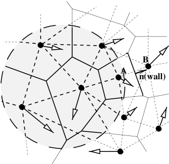
Figure 2: Voronoi and Delaunay tessellations of a 2D set of particles (filled circles). The solid lines form the Voronoi tessellation, the dashed lines the Delaunay tessellation. We also indicated a normal vector n of the wall separating the points ${\bf A}$ and ${\bf B}$. The grey circle represents the area in which one determines the top-hat filtered volume average of the velocity gradients. Courtesy: F. Bernardeau (see Bernardeau et al. 1997)

The Voronoi method defined in this way is based on the assumption that the field is uniform within each Voronoi cell of the tessellations, such that the field value throughout each of the Voronoi polyhedra is equal to that of the sample point of the tessellation (see Fig. 2 for a summarizing illustration of the method). Basically, the Voronoi cells are the multidimensional generalization of the bins in a 1-D zeroth-order interpolation scheme in which the function value is supposed to be constant within the interval centered on the sampling points, their value equal to that of the respective sample point values. Bernardeau & Van de Weygaert (1996) showed its great performance in the case of evaluating cosmic velocity fields. They showed the method to be of particular benefit when considering the gradient fields of discretely sampled fields rendered by the Voronoi method. In such situations, the Voronoi method yields a spatial geometry in which non-zero values of the field gradients are solely localized to the (polygonal) Voronoi walls. For the specific case of the window function for the volume filtering being a top-hat filter, the subsequent computation of the volume averages of the field gradients consist of a relatively simple sum of the values of those field gradients in each of the tessellation walls $k$ intersected or inside the filter sphere weighted by the surface area $A_{k}$ of the part of the wall located within the sphere.

The specific application to the statistics of the velocity divergence field $\nabla\cdot{\bf v}$ was shown to be very succesfull, corroborating the prediction of analytical perturbation theory considerations from a set of N-body simulations of structure formation (Bernardeau & Van de Weygaert 1996). Notwithstanding its virtues, the Voronoi method evidently represents an artificial situation in which the reconstructed fields are emphatically discontinous. Moreover, it cannot be applied to filter radii that are smaller than the average Voronoi wall distance. Below those scales the probability that a randomly placed filter sphere does not contain or intersect any Voronoi wall gets prohibitively high, and yielding unrealistic zero values for the field gradients.

In the one-dimensional situation a first-order improvement concerns the linear interpolation between the sampling points, leading to a fully continuous field. The natural extension to a multidimensional linear interpolation interval then immediately implies the corresponding Delaunay tessellation (Delone 1934). This tessellation (Fig. 1) consists of a volume-covering tiling of space into tetrahedra (in 3-D, triangles in 2-D, etc.) whose vertices are formed by four specific points in the dataset. The four points are uniquely selected such that their circumscribing sphere does not contain any of the other datapoints. The Voronoi and Delaunay tessellation are intimately related, being each others dual in that the centre of each Delaunay tetrahedron’s circumsphere is a vertex of the Voronoi cells of each of the four defining points, and conversely each Voronoi cell nucleus a Delaunay vertex (see Fig. 1). The “minimum triangulation” property of the Delaunay tessellation has in fact been well-known and abundantly applied in, amongst others, surface rendering applications such as geographical mapping and various computer imaging algorithms. Consider a set of ${\rm N}$ discrete datapoints in a finite region of M-dimensional space. Having at one’s disposal the field values at each of the $(1\!+\!{\rm M})$ Delaunay vertices ${\bf x}_{0},\ldots,{\bf x}_{\rm M}$, at each location ${\bf x}$ in the interior of a Delaunay M-dimensional tetrahedron the linear interpolation field value is determined by the estimated constant field gradient within the tetrahedron, $\,\,f({\bf x})~{}=~{}f({\bf x}_{0})~{}+~{}(\nabla f)|_{\rm Del}\!\!\!\cdot({\bf x}-{\bf x}_{0})\,\,\,$. Given the $(1\!+\!{\rm M})$ field values $f({\bf x}_{i})$, the value of the ${\rm M}$ components of the Delaunay field gradient $~{}(\nabla f)|_{\rm Del}$ can be computed straightforwardly by solving this linear relation for each of the ${\rm M}$ points ${\bf x}_{1},\ldots,{\bf x}_{\rm M}$.

This multidimensional Delaunay procedure of linear interpolation was introduced and described by Bernardeau & Van de Weygaert (1996) in the context of defining procedures for volume-weighted estimates of cosmic velocity fields. As they specifically focussed on the statistics of the velocity field gradients, in essence they defined a velocity gradient field of constant gradient values within each individual Delaunay tetrahedron, its value set by the measured velocity values at each of the 4 Delaunay vertices. They showed the superior performance of the first-order Delaunay estimator in reproducing analytical predictions of gravitational instability perturbation theory. The virtues and promise of the Delaunay method is in particularly underlined by its ability to unequivocally estimate the cosmic density parameter $\Omega$ on the basis of the particle velocities in the various N-body simulations of cosmic structure formation (Bernardeau etal. 1997).

     

Figure 3: A 9-frame mosaic comparing the performance of the Delaunay density estimating technique with a conventional grid-based TSC method in analyzing a cosmological N-body simulation. Left column: the particle distribution in a $10h^{-1}\hbox{Mpc}$ wide central slice through the simulation box. Central column: the corresponding Delaunay density field reconstruction. Right column: the TSC rendered density field reconstruction. The density grey scale is logarithmic, $\delta\rho/\rho=0-2400$.

4 Delaunay Density Field Estimation

The one factor complicating a trivial and direct implementation of above procedure in the case of density (intensity) field estimates is the fact that the number density of data points itself is the measure of the underlying density field value. We therefore cannot start with directly available field estimates at each datapoint. Instead, we need to define appropriate estimates from the point set itself. Most suggestive would be to base the estimate of the density field at the location ${\bf x}_{i}$ of each point on the inverse of the volume ${\rm V_{Vor,i}}$ of its Voronoi cell, $\rho({\bf x}_{i})\!=\!{\rm m}/{\rm V_{Vor,i}}$. Note that in this we take every datapoint to represent an equal amount of mass ${\rm m}$. The resulting field estimates are then intended as input for the above Delaunay interpolation procedure. However, one can demonstrate that integration over the resulting density field would yield a different mass than the one represented by the set of sample points (see Schaap & Van de Weygaert 2000a,b for a more specific and detailed discussion). Instead, mass conservation is naturally guaranteed when the density estimate is based on the inverse of the volume ${\rm W_{Vor,i}}$ of the “contiguous” Voronoi cell of each datapoint, $\rho({\bf x}_{i})\!\propto\!1/{\rm W_{Vor,i}}$. The “contiguous” Voronoi cell of a point is the cell consisting of the agglomerate of all $K$ Delaunay tetrahedra containing point $i$ as one of its vertices, whose volume ${\rm W_{Vor,i}}=\sum_{j=1}^{K}{\rm V_{Del,j}}$ is the sum of the volumes ${\rm V_{Del,j}}$ of each of the $K$ Delaunay tetrahedra. Properly normalizing the mass contained in the reconstructed density field, taking into account the fact that each Delaunay tetrahedron is invoked in the density estimate at $1\!+\!{\rm M}$ locations, we find at each datapoint the following density estimate, $\rho({\bf x}_{i})={\rm{m\,(1\!+\!M)}}/{\rm W_{Vor,i}}$. Having computed these density estimates, we subsequently proceed to determine the complete volume-covering density field reconstruction through the linear interpolation procedure outlined above.

The outstanding performance of our Delaunay Density Estimtor is illustrated by Figure 3 (see Schaap & Van de Weygaert 2000a), in which its performance on an N-body simulation of cosmic structure formation is compared with that of a conventional grid-based TSC technique. Cosmological N-body simulations provide an ideal template for illustrating the virtues of our method. They tend to contain a large variety of objects, with diverse morphologies, a large reach of densities, spanning over a vast range of scales. They display low density regions, sparsely filled with particles, as well as highly dense and compact clumps, represented by a large number of particles. Moderate density regions typically include strongly anisotropic structures such as filaments and walls. A comparison of the lefthand and righthand columns with the central column, i.e. the Delaunay estimated density fields, reveals the striking improvement rendered by our new procedure. Going down from the top to the bottom in the central column, we observe seemingly comparable levels of resolved detail. The self-adaptive skills of the Delaunay reconstruction evidently succeed in outlining the full hierarchy of structure present in the particle distribution, at every spatial scale represented in the simulation. The contrast with the achievements of the fixed grid TSC method in the righthand column is striking, in particular when focus tunes in on the finer structures. The central cluster appears to be a mere featureless blob! In addition, low density regions are rendered as slowly varying regions at moderately low values. This realistic conduct should be set off against the erratic behaviour of the TSC reconstructions, plagued by annoying shot-noise effects. Figure 3 also bears witness to the additional success of the Delaunay Estimator in reproducing sharp, edgy and clumpy filamentary and wall-like features. Automatically it resolves the fine details of their anisotropic geometry, seemlessly coupling sharp contrasts along one or two compact directions with the mildy varying density values along the extended direction(s). Moreover, it also manages to deal succesfully with the substructures residing within these structures. The well-known poor operation of e.g. the TSC method is clearly borne out by the central righthand frame. Its fixed and inflexible “filtering” characteristics tend to blur the finer aspects of such anisotropic structures. Such methods are therefore unsuited for an objective and unbiased scrutiny of the foamlike geometry which so pre-eminently figures in both the observed galaxy distribution as well as in the matter distribution in most viable models of structure formation.

Evidently, unlike artificial tailor-made methods, the Delaunay Density Estimator is sensitive in a fully self-consistent and self-adaptive fashion to intrinsically important structural elements. This provides ample arguments for its promise in great many astrophysical environments.

References

- [1] Bernardeau, F., van de Weygaert, R. (1996). MNRAS 279, 693–711
- [2] Bernardeau, F., van de Weygaert, R., Hivon, E., Bouchet, F. (1997). MNRAS 290, 566-576
- [3] Delone, B.N. (1934). Bull. Acad. Sci. USSR: Classe Sci. Mat. 7, 793
- [4] Icke, V., Van de Weygaert, R. (1987). Astron. Astrophys. 184, 1–9
- [5] Schaap, W., Van de Weygaert, R. (2000a). Astron. Astrophys. (submitted).
- [6] Schaap, W., Van de Weygaert, R. (2000b). Astron. Astrophys. (in prep).
- [7] Van de Weygaert, R. (1991) Ph.D. thesis, Leiden University, 1991
- [8] Van de Weygaert, R. (1994) Astron. Astrophys. 283, 361–406