How to fool CMB parameter estimation

Abstract

With the release of the data from the Boomerang and MAXIMA-1 balloon flights, estimates of cosmological parameters based on the Cosmic Microwave Background (CMB) have reached unprecedented precision. In this paper I show that it is possible for these estimates to be substantially biased by features in the primordial density power spectrum. I construct primordial power spectra which mimic to within cosmic variance errors the effect of changing parameters such as the baryon density and neutrino mass, meaning that even an ideal measurement would be unable to resolve the degeneracy. Complementary measurements are necessary to resolve this ambiguity in parameter estimation efforts based on CMB temperature fluctuations alone.

98.70.Vc,98.80.Es

I Introduction

With the release of the Boomerang[1] and MAXIMA-1[2] data sets, the promise of using the Cosmic Microwave Background to provide precision constraints on cosmological parameters has become a reality. The inflationary prediction of a flat universe has received spectacular confirmation, and remarkably good estimates of other cosmological parameters have emerged[3, 4]. More detailed observations of the CMB, in particular NASA’s MAP satellite[5] and the ESA’s Planck Surveyor[6], should allow for exquisitely precise determination of a handful of “fundamental” cosmological parameters such as the baryon density and the Hubble constant.

However, current parameter estimation efforts based on observation of the CMB suffer from an inherent ambiguity: lack of knowledge about the primordial density fluctuation spectrum. Primordial density and gravity wave fluctuations are the underlying source of the fluctuations in the CMB. The ability to predict the form of the CMB temperature anisotropy depends on knowledge of the form of these fluctuations. The standard assumption is that the density fluctuation power spectrum is a featureless power law, $P\left(k\right)\propto k^{n}$. Such an assumption is theoretically supported by inflation, which predicts such a power law spectrum. It is also empirically supported by observation of large scale structure. Current large scale structure data, however, only loosely constrain the form of the primordial power spectrum on scales relevant for CMB anisotropy measurements, $k\leq 0.1\,h\,{\rm MpC}^{-1}$[7]. A fully empirical approach to the data forces one to consider an arbitrary density power spectrum as input to the parameter estimation problem. This in effect adds so many free parameters (and associated degeneracies) that precision determination of parameters from the CMB temperature anisotropy alone becomes an impossibility. In this paper I expicitly construct primordial power spectra that mimic the effects of changes in cosmological parameters to within cosmic variance errors, meaning that even a perfect measurement of the CMB temperature fluctuations would be unable to resolve the degeneracy. This requires large deviations from the standard scale-invariant power law spectrum, $\delta P(k)/P(k)\sim 0.5$, which would be detectable with complementary measurements, such as CMB polarization and improved large-scale structure data like that from the Sloan Digital Sky Survey[8].

II The primordial power spectrum and the CMB

All observations of the CMB anisotropy published to date have been maps of the anisotropy in the temperature of the CMB, $\Delta T/T_{0}\sim 10^{-5}$, where $T_{0}=2.728\,{\rm K}$. It is convenient to quantify these temperature fluctuations as a set of multipole moments,

$${\delta T\left(\theta,\phi\right)\over T_{0}}=\sum_{\ell=0}^{\infty}\sum_{m=-\ell}^{\ell}{a_{\ell m}Y_{\ell m}\left(\theta,\phi\right)}.$$ (1)

Lack of a preferred direction implies that the amplitudes $a_{\ell m}$ will be independent of $m$,

$$\left\langle a^{*}_{\ell^{\prime}m^{\prime}}a_{\ell m}\right\rangle=C_{\ell}\delta_{\ell\ell^{\prime}}\delta_{mm^{\prime}},$$ (2)

where the angle brackets denote an average over realizations. For Gaussian fluctuations, the set of $C_{\ell}$’s completely characterizes the temperature anisotropy. If the fluctuations are non-Gaussian, higher order correlation functions are necessary to fully characterize the anisotropy. The power of the CMB in constraining cosmological parameters comes from the fact that one is using a large number of parameters (the $C_{\ell}$ spectrum) to constrain a dozen or so “fundamental” parameters such as the baryon density, the ratio of gravity wave perturbations to density perturbations, and so on. Any given CMB observation will have access to a range of $C_{\ell}$’s with error bars determined by a combination of the observation’s sky coverage, sensitivity and angular resolution. However, there exists a fundamental limit to the accuracy with which the $C_{\ell}$ spectrum can be measured, referred to as cosmic variance,

$${\Delta C_{\ell}\over C_{\ell}}\geq\sqrt{1\over 2\ell+1}.$$ (3)

Cosmic variance is simply a finite sample size effect coming from the fact that there is only a single sky to measure, and is more significant at long wavelength (smaller $\ell$). Cosmic variance will play a central role in the discussion below for the reason that any two $C_{\ell}$ spectra which have a small enough $\chi^{2}$ over cosmic variance errors are in principle indistinguishable, even when subject to an ideal measurement.

Going from a $C_{\ell}$ spectrum to cosmological parameters requires assumptions about the form of the density power spectrum. A typical assumption when discussing the ability to constrain cosmological parameters using the CMB is that the primordial density power spectrum is a power law:

$$P\left(k\right)\propto k^{n},$$ (4)

where the spectral index $n$ is close to the scale-invariant value $n=1$. The recent Boomerang measurement[3] yields a value $n=0.87^{+0.11}_{-0.08}$ for a set of priors consistent with inflation, and the MAXIMA-1 measurement has a best fit of $n=0.99\pm 0.09$[4]. Such a featureless power law spectrum is in fact predicted by most inflationary models. A natural extension of this approximation is to allow “running” of the spectral index,

$${dn\over d\log k}\neq 0.$$ (5)

Such running is a feature of some inflation models[9, 10, 11, 12, 13, 14]. Future CMB observations will be able to detect running of the spectral index as small as $dn/d\log\left(k\right)\simeq 0.05$[11]. Taking this a step further, Lesgourges, Prunet and Polarski considered CMB constraints on models with broken scale invariance[15]. In principle, however, the primordial power spectrum can contain many more free parameters than just one or two. The purpose of this paper is to investigate the possibility that features in the primordial power spectrum could mimic the effect of other parameters and thus “fool” parameter estimation efforts which assume a featureless power law spectrum. It is to be expected that such confusion will be possible, since the number of parameters available in an arbitrary primordial power spectrum is much larger than the parameter space considered by typical parameter estimation efforts, and can in principle be larger than the number of multipoles available in the CMB for measurement. I show below that the number of free parameters necessary to confuse parameter estimation efforts is fewer than a hundred. In the next section I discuss the numerical methods used to approach the problem.

III Numerical methods

Boltzmann codes for calculating the CMB spectrum normally take a set of cosmological parameters as input and generate a spectrum of $C_{\ell}$’s. In this paper I construct primordial power spectra which would cause significant mis-estimation of parameters if a power law fluctuation spectrum were to be assumed in the likelihood analysis. This amounts to solving the inverse problem – given a particular $C_{\ell}$ spectrum, what primordial power spectrum is necessary to produce it? I adopt a simple $\chi^{2}$ minimization procedure for solving this problem. The procedure is as follows.

I choose two models and generate CMB multipole spectra for each using the CMBFAST code[16]. One I call the “true” model, with a set of parameters assumed to represent the actual underlying cosmos. The second I call the “target” model, generated with a different set of parameters but the same density power spectrum, which I take to be the scale invariant spectrum $P\left(k\right)\propto k$. The goal is to deform the density power spectrum in such a way as to mimic the $C_{\ell}$ spectrum of the target model while retaining the underlying parameters of the true model. The observer will see the target spectrum, but the true parameters of the universe are those of the true model. The input power spectrum is binned into $N_{k}=75$ bins $i$ with wavenumber $k_{i}$. This binning provides a good balance between accuracy and computational efficiency. CMBFAST samples the power spectrum at a much higher resolution, so the binned data is smoothed using cubic spline interpolation[17]. The “trial” density power spectrum $P^{\rm trial}\left(k\right)$ is initially a power law and is adjusted iteratively until the trial CMB spectrum $C^{\rm trial}_{\ell}$ matches the target CMB spectrum $C^{\rm target}_{\ell}$ to within cosmic variance errors. The first step is to numerically calculate a correlation matrix between the $C_{\ell}$’s and the primordial power spectrum

$$D_{i\ell}\equiv{\partial C^{\rm trial}_{\ell}\over\partial P\left(k_{i}\right)},$$ (6)

where $k_{i}$ is the wavenumber of the $i$’th bin and $P\left(k_{i}\right)$ is the amplitude of the density power spectrum at that scale. Note that this is not a square matrix: $\ell=1,\ldots N_{\ell}$ and $i=1,\ldots,N_{k}$. I use $N_{k}=75$ and $N_{\ell}=1500$. It is also necessary to compute the derivative of the $\chi^{2}$ between the trial and target spectra:

$${\partial\chi^{2}\over\partial P\left(k_{i}\right)}= {\partial\over\partial P\left(k_{i}\right)}\sum_{\ell}{\left[{C^{\rm trial}_{\ell}-C^{\rm target}_{\ell}\over\sigma_{\ell}}\right]^{2}}$$ (7)

$$= 2\sum_{\ell}{D_{i\ell}{\left[C^{\rm trial}_{\ell}-C^{\rm target}_{\ell}\right]\over\sigma_{l}^{2}}}.$$ (8)

I take the errors to be the cosmic variance limit

$$\sigma_{\ell}=\sqrt{1\over 2\ell+1}C^{\rm target}_{\ell}.$$ (9)

This is particularly important: any two spectra that agree within cosmic variance limits are impossible to distinguish with any CMB measurement, no matter how sensitive. The result is therefore independent of any particular experiment. A new density power spectrum is calculated by gradient descent[18]:

$$P^{\rm new}\left(k_{i}\right)=P^{\rm trial}\left(k_{i}\right)-\lambda\sum_{j=1}^{N_{k}}{\alpha^{-1}_{ij}{\partial\chi^{2}\over\partial P\left(k_{j}\right)}},$$ (10)

where $\lambda$ is a constant whose value is picked to ensure smooth convergence (I use $\lambda=0.1$), and the matrix $\alpha_{ij}$ is defined in terms of the derivative matrix (6) as:

$$\alpha_{ij}\equiv\sum_{\ell=1}^{N_{\ell}}{{1\over\sigma_{l}^{2}}D_{i\ell}D_{j\ell}}.$$ (11)

Inversion of the matrix $\alpha_{ij}$ is in practice somewhat problematic, as the matrix is in numerically singular. Typically only half of the 75 eingenvalues of the matrix are finite. I use singular value decomposition methods to perform the inversion[19]. Once a new $P^{\rm trial}$ is generated, the procedure is iterated until an acceptable $\chi^{2}$ is achieved, which I define to be $\chi^{2}<100$, more than good enough to make the spectra indistinguishable in practice. Convergence typically requires around 20 iterations. In the next section I describe the results of the calculations.

IV Results and Conclusions

I choose a target model that is a good fit to the Boomerang and MAXIMA-1 observations, with the following parameters:

$$\Omega_{\rm total}=1$$ (12)

$$\Omega_{\rm b}h^{2}=0.027$$ (13)

$$\Omega_{CDM}=0.3$$ (14)

$$\Omega_{\Lambda}=0.645$$ (15)

$$\Omega_{\nu}=0$$ (16)

$$h=0.7$$ (17)

$$n=1$$ (18)

$$\tau=0.2$$ (19)

$$r=0$$ (20)

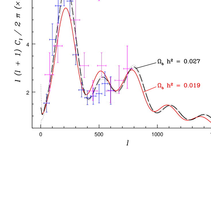
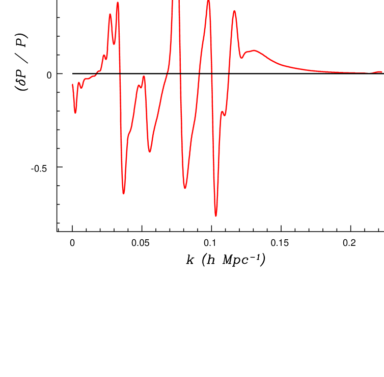
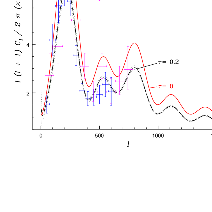
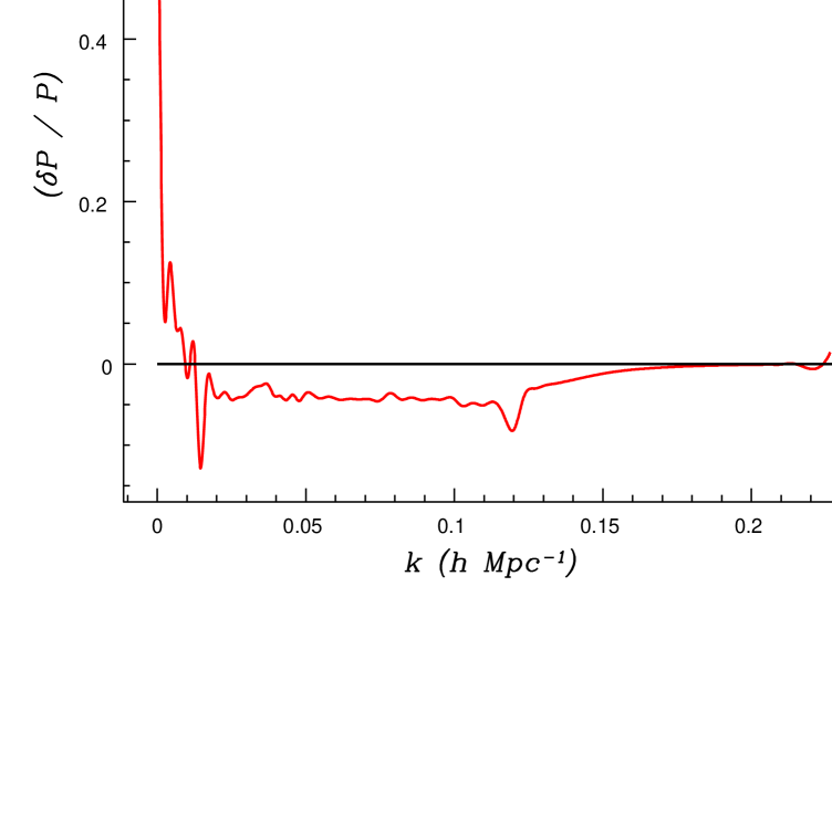
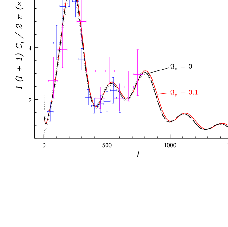
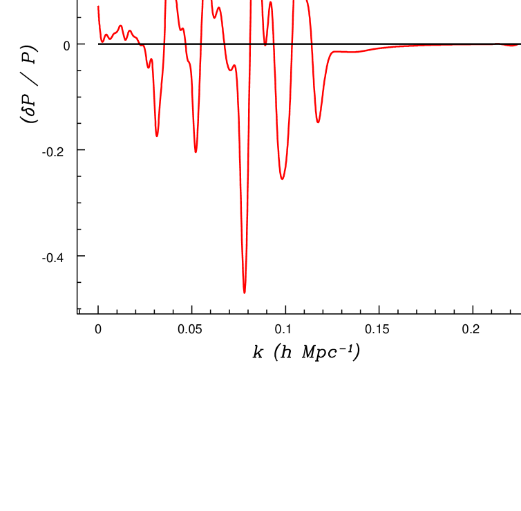
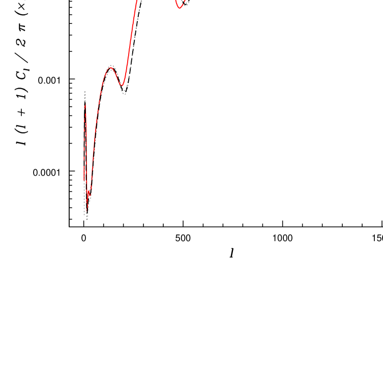
Here $h$ is the Hubble constant in units of $100\,{\rm km/s}$, $n$ is the scalar spectral index, $\tau$ is the reionization optical depth, and $r$ is the tensor/scalar ratio. The procedure is to change one or more of the parameters of the target model to produce a “true” model, then reproduce the $C_{\ell}$ spectrum of the target model by modifying the underlying matter power spectrum as described in Section III. This choice of target model has two peculiarities. First, the baryonic density is outside the range preferred by Big Bang Nucleosynthesis (BBN), $\Omega_{\rm b}h^{2}=0.019\pm 0.0024$[20, 21]. Second, the reionization optical depth is large, $\tau=0.2$. Figure 1 shows the target $C_{\ell}$ spectrum and the $C_{\ell}$ spectrum resulting from setting $\Omega_{\rm b}h^{2}=0.019$ in accordance with BBN limits. The power spectrum necessary to change the $C_{\ell}$ spectrum of the true model into one indistinguishable from that of the target model is shown in Figure 2. The perturbation to the power spectrum is quite large, and would be difficult to produce via inflation. However, such a power spectrum is in principle allowed by existing data. Another choice is to change the reionization optical depth $\tau$ instead of the baryon density. Fig. 3 shows the target model and a model with $\tau=0$. The power spectrum required for the true model to mimic the target model is shown in Figure 4. In this case, the power spectrum is dominated by a single large feature at long wavelength, a situation that could potentially be realized within an inflationary context. Finally, Figures 5 and 6 show the results with $\Omega_{\nu}=0.1$, corresponding to a neutrino mass of $m_{\nu}=4.5\,{\rm eV}$.

It is clear that allowing for an arbitrary density power spectrum renders attempts at parameter estimation from the CMB temperature anisotropy alone a hopeless task. It is necessary to use complementary measurements to constrain the density power spectrum. If measurements of the CMB polarization are available in addition to measurements of the temperature anisotropy, the task of “fooling” CMB parameter estimation efforts becomes much more difficult. Polarization is a tensor quantity, which can be decomposed on the celestial sphere into “electric-type”, or scalar, and “magnetic-type”, or pseudoscalar modes. The symmetric, trace-free polarization tensor ${\cal P}_{ab}$ can be expanded as[22]

$${{\cal P}_{ab}\over T_{0}}=\sum_{\ell=0}^{\infty}\sum_{m=-\ell}^{\ell}\left[a^{E}_{\ell m}Y^{E}_{\left(\ell m\right)ab}\left(\theta,\phi\right)+a^{B}_{\ell m}Y^{B}_{\left(\ell m\right)ab}\left(\theta,\phi\right)\right],$$ (21)

where the $Y^{E,B}_{\left(\ell m\right)ab}$ are electric- and magnetic-type tensor spherical harmonics, with parity $(-1)^{\ell}$ and $(-1)^{\ell+1}$, respectively. Unlike a temperature-only map, which is described by the single multipole spectrum of $C^{T}_{\ell}$’s, a temperature/polarization map is described by three spectra

$$\left\langle\left|a^{T}_{\ell m}\right|^{2}\right\rangle\equiv C_{T\ell},\ \left\langle\left|a^{E}_{\ell m}\right|^{2}\right\rangle\equiv C_{E\ell},\ \left\langle\left|a^{B}_{\ell m}\right|^{2}\right\rangle\equiv C_{B\ell},$$ (22)

and three correlation functions,

$$\left\langle a^{T*}_{\ell m}a^{E}_{\ell m}\right\rangle\equiv C_{C\ell},\ \left\langle a^{T*}_{\ell m}a^{B}_{\ell m}\right\rangle\equiv C_{(TB)\ell},\ \left\langle a^{E*}_{\ell m}a^{B}_{\ell m}\right\rangle\equiv C_{(EB)\ell}.$$ (23)

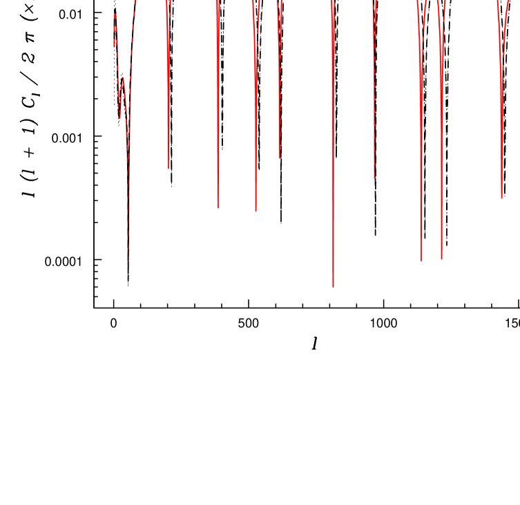
Parity requires that the last two correlation functions vanish, $C_{(TB)\ell}=C_{(EB)\ell}=0$, leaving four spectra: temperature $C_{T\ell}$, E-mode $C_{E\ell}$, B-mode $C_{B\ell}$, and the cross-correlation $C_{C\ell}$. Since scalar density perturbations have no “handedness,” it is impossible for scalar modes to produce B-mode (pseudoscalar) polarization. Only tensor fluctuations (or foregrounds [23]) can produce a B-mode. In the cases I have considered in this paper, calculation of the polarization spectra reveals that models with indistinguishable temperature fluctuations have very distinct patterns of polarization, so that a sufficiently sensitive measurement of the polarization power spectra (such as that which will be produced by the Planck satellite) would reveal any inconsistency in the assumption of a power-law density fluctuation spectrum. Figure 7 shows the E-mode polarization spectra for the case considered in Fig. 1, in which the baryon density is varied. Fig. 8 shows the cross-correlation spectrum $C_{T\ell}$ for the same case. The B-mode vanishes. Table I shows the $\chi^{2}$ over cosmic variance errors for all three CMB multipole spectra (temperature, E-mode and cross-correlation) for the models considered in this paper. In all three cases, although it is possible to mimic the $C_{T\ell}$ spectrum of the target model to within cosmic variance, the polarization spectra produced are poor fits to the respective target polarization spectra. Additional information on the density power spectrum can be obtained from large scale structure data. The prostpect for independent constraint of the density power spectrum from a combination of SDSS data and CMB polarization was considered by Wang et al.[24].

Model	$\chi^{2}$: Temperature	$\chi^{2}$: E-mode	$\chi^{2}$: cross-correlation
$\Omega_{\rm b}h^{2}=0.019$, $\Omega_{\Lambda}=0.661$	$80$	$2.2\times 10^{5}$	$4.9\times 10^{7}$
$\tau=0$	$76$	$500$	$2.1\times 10^{4}$
$\Omega_{\nu}=0.1$, $\Omega_{\Lambda}=0.545$	$97$	$3.5\times 10^{4}$	$1.8\times 10^{7}$

TABLE I.: $\chi^{2}$ for various model fits, relative to cosmic variance errors over $N_{\ell}=1500$ multipole moments. All $\chi^{2}$ values are calculated relative to the target model, with $\Omega_{\rm b}h^{2}=0.027$, $\Omega_{\Lambda}=0.645$, and $\tau=0.2$. $\Omega_{\rm total}=1$ in all cases. While the temperature multipole spectra are excellent fits, the fits of the polarization spectra are poor.

In this paper I have shown by construction that it is possible to mimic the effect of changes in fundamental cosmological parameters on the CMB by changes in the density power spectrum. With a $N_{k}=75$ parameter fit of the power spectrum, a CMB multipole spectrum with significantly shifted parameters can be fit to within cosmic variance errors, so that even an ideal measurement would be unable to resolve the degeneracy. It is therefore possible for estimates of cosmological parameters based on CMB temperature fluctuations alone to be substantially biased by features in the density power spectrum. This degeneracy cannot be resolved without access to complementary measurements such as observation of CMB polarization or information about large scale structure such as that which will be provided by the Sloan Digital Sky Survey.