MULTICHANNEL INTERFERENCE MITIGATION TECHNIQUES IN RADIO ASTRONOMY

Abstract

Radio-astronomical observations are increasingly corrupted by RF interference, and online detection and filtering algorithms are becoming essential. To facilitate the introduction of such techniques into radio astronomy, we formulate the astronomical problem in an array signal processing language, and give an introduction to some elementary algorithms from that field. We consider two topics in detail: interference detection by rank estimation of short-term covariance matrices, and spatial filtering by subspace estimation and projection. We discuss experimental data collected at the Westerbork radio telescope, and illustrate the effectiveness of the space-time detection and blanking process on the recovery of a 3C48 absorption line in the presence of GSM mobile telephony interference.

./figures/

1 INTRODUCTION

Radio-astronomical observations are increasingly corrupted by RF interferers such as wireless communication and satellite navigation signals. Online detection and filtering algorithms are essential to reduce the effect of interference to an acceptable level. However, existing methods have a limited scope. Until now, the most widely implemented algorithm is a single-channel total power change detector, followed by a blanking of the correlator output. Friedman [3] has implemented an improved power detector at the RATAN600, based on detection of change in the power. Weber et al. [17] proposed the use of the quantized correlation at all lags to test the presence of interference. Another detector based on wavelet decomposition has been proposed by Maslakovic et al. [12]. These are all single channel detectors which do not exploit the spatial properties of the interference. The only detector which considered combining multiple telescopes for improved detection and blanking was proposed by Kasper Chute $\&$ Routledge [6] for low frequency interferometry, where a robust data censoring method based on the temporal behavior of the cross spectrum was proposed. This requires a large number of estimated spectra ($10^{5}$) to obtain reliable robust estimates, and only two channels are used. Finally, adaptive filtering techniques have recently been considered by Barnbaum $\&$ Bradley [1] who propose to excise interference from the Green-Bank radio telescope using a reference antenna and an LMS type algorithm.

Our aim in this paper is to introduce modern array signal processing techniques to the context of radio astronomy, and to investigate the merits of multichannel detection and filtering algorithms at the Westerbork Synthesis Radio Telescope (WSRT). By combining cross-correlation information of a large number of sensor pairs, we can increase the detection performance significantly, and also estimate the spatial signature of interferers. In essence, our approach is to compute (on-line) short-term spatial correlation matrices in narrow sub-bands, and then to compute the eigenvalue decomposition of each of these matrices [11]. A rank estimate based on the eigenvalues allows to detect the number of interfering signals in each time-frequency slot, and the dominant eigenvectors give information on the “spatial signature” of the interferers.

After detection, we can follow two directions. We can reduce the interference by rejecting corrupted time-frequency slots (blanking). This approach is suitable for time-slotted communication signals such as the European mobile telephony standard GSM, or the TDMA (time-division multiple access)-based mobile telephony standards IS-54/136 in the US.

A more challenging approach is to also use the eigenvector information. Indeed, we can project out those dimensions in the spatial correlation matrices that correspond to the spatial signature vectors of the interference. Such spatial filtering techniques will greatly enhance the performance of observations with continuously-present interference.

The effectiveness of the space-time detection and blanking process is demonstrated by applying the algorithms to data measured at the WSRT using an on-line 8-channel recording system. As will be shown in section 7, we were able to recover an absorption line of 3C48 which was completely masked by a superimposed GSM interference, and could not be recovered by single channel techniques.

The paper is written in a tutorial style, to appeal to both the radio astronomy and the signal processing communities. The structure of the paper is as follows. After posing the astronomical measurement equations in section 2, we reformulate the model in terms of array processing matrix language in section 3. We then introduce RF interference and describe its effect on the received data. In section 5 we discuss various detection algorithms. We compare the single and multichannel detectors, for the case of a narrow-band interferer with known spatial signature vector, and then present two multichannel detectors that do not assume this knowledge. We then move to spatial filtering techniques in section 6, where we formulate the basic ideas and describe a projections based approach. Finally, experimental results on multichannel blanking are shown in section 7.

2 ASTRONOMICAL MEASUREMENT EQUATIONS

In this section we briefly describe a simplified mathematical model for the astronomical measurement process. Our discussion follows the introduction in Perley Schwab $\&$ Bridle [14]. The purpose of this is to connect to a matrix formulation commonly used in array signal processing, in the next section.

The signals received from the celestial sphere may be considered as spatially incoherent wideband random noise. It is possibly polarized and perhaps contains spectral absorption or emission lines. Rather than considering the emitted electric field at a location on the celestial sphere, astronomers try to recover the intensity (or brightness) $I_{f}(\mathbf{s})$ in the direction of unit-length vectors $\mathbf{s}$, where $f$ is a specific frequency. Let $E_{f}(\mathbf{r})$ be the received celestial electric field at a location $\mathbf{r}$ on earth (see figure 1$(a)$). Assume that the telescopes are identical, and let $A(\mathbf{s})$ denote the amplitude response of a telescope to a source in the direction $\mathbf{s}$. The measured correlation of the electric fields between two sensors $i$ and $j$ with locations $\mathbf{r}_{i}$ and $\mathbf{r}_{j}$ is called a visibility and is (approximately) given by [Perley Schwab $\&$ Bridle [14]]

$$V_{f}(\mathbf{r}_{i},\mathbf{r}_{j}):={\rm E}\{E_{f}(\mathbf{r}_{i})\overline{E_{f}(\mathbf{r}_{j})}\}\;=\;\int_{\hbox{\small sky}}A^{2}(\mathbf{s})I_{f}(\mathbf{s})e^{-j2\pi f\;\mathbf{s}^{T}(\mathbf{r}_{i}-\mathbf{r}_{j})/c}\;d\Omega\,.$$

(${\rm E}\{\,\cdot\,\}$ is the mathematical expectation operator, the superscript ^T denotes the transpose of a vector, and overbar denotes the complex conjugate.) Note that it is only dependent on the oriented distance $\mathbf{r}_{i}-\mathbf{r}_{j}$ between the two telescopes; this vector is called a baseline.

For simplification, we may sometimes assume that the astronomical sky is a collection of $d$ discrete point sources (maybe unresolved). This gives

$$I_{f}(\mathbf{s})=\sum_{n=1}^{d}I_{f}(\mathbf{s}_{n})\delta(\mathbf{s}-\mathbf{s}_{n})\,,$$

where $\mathbf{s}_{n}$ is the coordinate of the $n$’th source, and thus

$$V_{f}(\mathbf{r}_{i},\mathbf{r}_{j})\;=\;\sum_{n=1}^{d}\,A^{2}(\mathbf{s}_{n})I_{f}(\mathbf{s}_{n})\,e^{-j2\pi f\,\mathbf{s}_{n}^{T}(\mathbf{r}_{i}-\mathbf{r}_{j})/c}\,.$$ (1)

Up to this point we have worked in an arbitrary coordinate system. For earth rotation synthesis arrays, a coordinate system is often introduced as follows. We assume an array with telescopes that have a small field of view and that track a reference source direction $\mathbf{s}_{0}$ in the sky. Other locations in the field of view can be written as

$$\mathbf{s}=\mathbf{s}_{0}+{\mbox{\boldmath$\sigma$}}\,,\qquad\mathbf{s}_{0}\perp{\mbox{\boldmath$\sigma$}}\,,$$

(valid for small $\sigma$) and a natural coordinate system is

$$\mathbf{s}_{0}=[0,\,0,\,1]^{T}\,,\qquad{\mbox{\boldmath$\sigma$}}=[\ell,\,m,\,0]^{T}\,.$$

Similarly, for a planar array, the receiver baselines can be parameterized as

$$\mathbf{r}_{i}-\mathbf{r}_{j}=\lambda[u,\,v,\,w]^{T}\,,\qquad\lambda=\displaystyle\frac{c}{f}\,.$$

The measurement equation in $(u,v,w)$ coordinates thus becomes

$$V_{f}(u,v,w)\;=\;e^{-j2\pi w}\int\!\!\!\int\;A^{2}(\ell,m)I_{f}(\ell,m)\,e^{-j2\pi(u\ell+vm)}\,d\ell dm\,.$$ (2)

The factor $e^{-j2\pi w}$ is caused by the geometrical delay associated to the reference location, and can be compensated by introducing a slowly time-variant delay (see figure 1$(b)$). This synchronizes the center of the field-of-view and makes the reference source location appear as if it was at the north pole. After compensation, we arrive at a measurement equation in $(u,v)$ coordinates only,

$$V_{f}(u,v)\;=\;\int\!\!\!\int\;A^{2}(\ell,m)I_{f}(\ell,m)\,e^{-j2\pi(u\ell+vm)}\,d\ell dm\,.$$ (3)

It has the form of a Fourier transformation.

The function $V_{f}(u,v)$ is sampled at various coordinates $(u,v)$ by first of all taking all possible sensor pairs $i,j$ or baselines $\mathbf{r}_{i}-\mathbf{r}_{j}$, and second by realizing that the sensor locations $\mathbf{r}_{i}$, $\mathbf{r}_{j}$ are actually time-varying since the earth rotates. Given a sufficient number of samples in the $(u,v)$ domain, the relation can be inverted to obtain an image (the ‘map’).

3 ARRAY SIGNAL PROCESSING FORMULATION

3.1 Obtaining the measurements

We will now describe the situation from an array signal processing point of view. The signals received by the telescopes are amplified and downconverted to baseband. A time-varying delay for every telescope is also introduced, to compensate for the geometrical delay.

Following traditional array signal processing practices, the signals at this point are called $x_{i}(t)$ rather than $E_{f}(\mathbf{r})$, and are stacked in vectors

$$\mathbf{x}(t)=\left[\begin{array}[]{c}x_{1}(t)\\ \vdots\\ x_{p}(t)\end{array}\right]\,,$$

where $p$ is the number of telescopes. These are then processed by a correlation stage.

It will be convenient to assume that $\mathbf{x}(t)$ is first split by a bank of narrow-band sub-band filters into a collection of frequency-components $\mathbf{x}_{f}(t)$. The main output of the telescope hardware is then a sequence of empirical correlation matrices $\mathbf{\hat{R}}_{f}(t)$ of cross-correlations of $\mathbf{x}_{f}(t)$, for a set of frequencies $f\in\{f_{k}\}$ covering a 10 MHz band or so, and for a set of times $t\in\{t_{k}\}$ covering up to 12 hours. Each correlation matrix $\mathbf{\hat{R}}_{f}(t)$ is an estimate of the true covariance matrix $\mathbf{R}_{f}(t)$,

$$\mathbf{R}_{f}(t)\;=\;{\rm E}\{\mathbf{x}_{f}(t)\mathbf{x}_{f}(t)^{\raisebox{1.0pt}{$\rm\scriptscriptstyle H$}}\}\,,\qquad\mathbf{\hat{R}}_{f}(t)=\frac{1}{N}\sum_{n=0}^{N-1}\mathbf{x}_{f}(t+nT)\mathbf{x}_{f}(t+nT)^{\raisebox{1.0pt}{$\rm\scriptscriptstyle H$}}\,,$$ (4)

where the superscript ${}^{\raisebox{1.0pt}{$\rm\scriptscriptstyle H$}}$ denotes a complex conjugate transpose, $T$ is the sample period of $\mathbf{x}_{f}(t)$ and $N$ is the number of samples over which is averaged. This is drawn schematically in figure 2 (ignoring the detection stage for the moment). The matrices $\mathbf{\hat{R}}_{f}(t)$ are stored for off-line spectral analysis and imaging.

Typically, the averaging period $NT$ is in the order of 10-30 s, whereas each sub-band has a bandwidth in the order of 100 kHz or less. Due to the sub-band filtering, the original sampling rate of $\mathbf{x}(t)$ is reduced accordingly, resulting in $T$ in the order of $10\ \mu$s.

The connection of the correlation matrices $\mathbf{R}_{f}(t)$ to the visibilities $V_{f}(u,v)$ in section 2 is as follows. Each entry $r_{ij}(t)$ of the matrix $\mathbf{R}_{f}(t)$ is a sample of this visibility function for a specific coordinate $(u,v)$, corresponding to the baseline vector $\mathbf{r}_{i}(t)-\mathbf{r}_{j}(t)$ between telescopes $i$ and $j$ at time $t$:

$$\mathbf{r}_{i}(t)-\mathbf{r}_{j}(t)=\lambda[u_{ij}(t),\;v_{ij}(t),\;w_{ij}(t)]$$

$$V_{f}(u_{ij}(t),v_{ij}(t))\equiv r_{ij}(t)\,.$$

Note that we can obtain only a discrete set of $(u,v)$ sample points. Indeed, the number of instantaneous independent baselines between $p$ antennas is less than $\frac{1}{2}p(p-1)$. Also, using the earth rotation, the number of samples $\{t_{k}\}$ is given by the ratio of the observation time and the covariance averaging time (e.g., 12 h/30 sec = 1440 samples).

A few remarks on practical issues are in order.

• Many telescope sites including WSRT follow actually a different scheme where the signals are first correlated at several lags and subsequently Fourier transformed. This leads to similar results.

• The geometrical delay compensation is usually introduced only at the back end of the receiver. At this point, also a phase correction is needed to compensate for the factor $e^{-j2\pi w_{ij}(t)}$ in the measurement equation (2). This is referred to as fringe correction [16]. Since the earth rotates, $w_{ij}(t)$ is slowly time varying, with a rate of change in the order of 0–10 Hz depending on source declination and baseline length.

3.2 Matrix formulation

For the discrete source model, we can now formulate our measurement equations in terms of matrices. Let $\mathbf{r}_{0}(t_{k})$ be an arbitrary and time-varying reference point, typically at one of the elements of the array, and let us take the $(u,v,w)$ coordinates of the other telescopes with respect to this reference,

$$\mathbf{r}_{i}(t)-\mathbf{r}_{0}(t)=\lambda[u_{i0}(t),\;v_{i0}(t),\;w_{i0}(t)]\,,\qquad i=1,\cdots,p\,.$$

Equation (1) can then be written slightly different as

$$\begin{array}[]{rcl}V_{f}(\mathbf{r}_{i}(t),\mathbf{r}_{j}(t))&=&\displaystyle\sum_{n=1}^{d}e^{-j2\pi f\,\mathbf{s}_{n}^{T}(\mathbf{r}_{i}-\mathbf{r}_{0})/c}\,A^{2}(\mathbf{s}_{n})I_{f}(\mathbf{s}_{n})\,e^{j2\pi f\,\mathbf{s}_{n}^{T}(\mathbf{r}_{j}-\mathbf{r}_{0})/c}\\ \Leftrightarrow\quad V_{f}(u_{ij}(t),v_{ij}(t))&=&\displaystyle\sum_{n=1}^{d}\par e^{-j2\pi(u_{i0}(t)\ell_{n}+v_{i0}(t)m_{n})}\,A(\ell_{n},m_{n})\cdot\\ &&\quad\quad I_{f}(\ell_{n},m_{n})\cdot A(\ell_{n},m_{n})\,e^{j2\pi(u_{j0}(t)\ell_{n}+v_{j0}(t)m_{n})}\,.\end{array}$$

In terms of correlation matrices, this equation can be written as

$$\mathbf{R}_{f}(t)\;=\;\mathbf{A}_{f}(t)\mathbf{B}_{f}\mathbf{A}^{\raisebox{1.0pt}{$\rm\scriptscriptstyle H$}}_{f}(t)$$ (5)

where

$$\mathbf{A}_{f}(t)=\left[\mathbf{a}_{t,f}(\ell_{1},m_{1}),\cdots,\mathbf{a}_{t,f}(\ell_{d},m_{d})\right]$$

and

$$\mathbf{a}_{t,f}(\ell,m)=\left[\begin{array}[]{c}e^{-j(u_{10}(t)\ell+v_{10}(t)m)}\\ \vdots\\ e^{-j(u_{p0}(t)\ell+v_{p0}(t)m)}\end{array}\right]A(\ell_{n},m_{n})$$ (6)

$$\mathbf{B}_{f}=\left[\begin{array}[]{ccc}I_{f}(\ell_{1},m_{1})&&\mbox{\bf 0}\\ &\ddots&\\ \mbox{\bf 0}&&I_{f}(\ell_{d},m_{d})\end{array}\right]$$

The vector function $\mathbf{a}_{t,f}(\ell,m)$ is called the array response vector in array signal processing. It describes the response of the telescope array to a source in the direction $(\ell,m)$. As usual, the array response is frequency dependent. In this case, the response is also slowly time-varying due to the earth rotation. Note, very importantly, that the function as shown here is completely known, since the beam shape $A(\ell,m)$ is calibrated and we know the locations of the telescopes very well.

More realistically, the array response is less perfect. An important effect is that each telescope may have a different complex receiver gain, $\gamma_{i}(t)$, dependent on many angle-independent effects such as cable losses, amplifier gains, and (slowly) varying atmospheric conditions. If we take this into account, the model now becomes

$$\mathbf{R}_{f}(t)\;=\;\mbox{$\mbox{\boldmath$\Gamma$}$}(t)\mathbf{A}_{f}(t)\mathbf{B}_{f}\mathbf{A}^{\raisebox{1.0pt}{$\rm\scriptscriptstyle H$}}_{f}(t)\mbox{$\mbox{\boldmath$\Gamma$}$}(t)$$

where

$$\mbox{$\mbox{\boldmath$\Gamma$}$}(t)=\left[\begin{array}[]{ccc}\gamma_{1}(t)&&\mbox{\bf 0}\\ &\ddots&\\ \mbox{\bf 0}&&\gamma_{p}(t)\end{array}\right]\,.$$

In future equations we will drop the dependence on $f$.

3.3 Additive noise

In reality, most of the received signal consists of additive system noise. When this noise is zero mean, independent among the antennas (thus spatially white), and identically distributed, then it has a covariance matrix that is a multiple of the identity matrix, $\sigma^{2}\mathbf{I}$, where $\sigma^{2}$ is the noise power on a single antenna inside the subband which we consider. Usually the noise is assumed to be Gaussian.

The resulting model of the received covariance matrix then becomes

$$\mathbf{R}(t)=\mbox{$\mbox{\boldmath$\Gamma$}$}(t)\mathbf{A}(t)\mathbf{B}\mathbf{A}^{\raisebox{1.0pt}{$\rm\scriptscriptstyle H$}}(t)\mbox{$\mbox{\boldmath$\Gamma$}$}(t)^{\raisebox{1.0pt}{$\rm\scriptscriptstyle H$}}+\sigma^{2}\mathbf{I}\,.$$ (7)

Note that this assumes that the noise is introduced after the varying receiver gains. This assumption is reasonable if the channels from the low-noise amplifier (LNA) outputs to the analog-to-digital converter (ADC) units are equal. Otherwise, it is still reasonable to assume that the noise is spatially white, i.e., the noise covariance matrix is diagonal. We can assume that it can be estimated using various calibration techniques; a simple diagonal scaling will then bring us back to the model (7). We further assumed that the quantization is fine, since a large dynamic range is needed to cope with strong interferers.

The study of factorizations of the spatial covariance matrices such as shown above is the key to many array signal processing techniques. The knowledge of the specific structure of the array response vector (6) is of course already used in radio astronomy, as it enables the construction of the map using inverse Fourier techniques. The main point in this paper is to demonstrate that also interference adds a specific structure to the covariance matrices. This hopefully will allow its detection, provided our models are sufficiently accurate.

4 RF INTERFERENCE

RF interference (RFI) usually enters the antennas through the sidelobes of the main beam. It can be stronger or weaker than the system noise. An important property is that it has a certain spatial signature, or array response vector, which becomes explicit in the case of narrow-band signals.

Examples of RFI present at WSRT are television broadcasts (Smilde station), geolocation satellites (GPS and Glonass), taxi dispatch systems, airplane communication and navigation signals, wireless mobile communication (GSM) and satellite communication signals (Iridium). Thus, interferers may be continuous or intermittent, narrow-band or wideband, and strong or weak. Some examples of actual interference are presented at the end of the section.

Interference is usually not stationary over 10 seconds (let alone because of the time-varying fringe rate of 0–10 Hz), and hence it might be argued that it would average out from the long-term correlations. However, the amount of nonstationarity is often insufficient to provide a good and reliable protection [15], [16].

4.1 Narrow-band interference model

Suppose that we have a single interferer impinging on the telescope array. The interfering signal reaches the array with different delays $\tau_{i}$ for each telescope. After demodulation to baseband, we have

$$x_{i}(t)=a_{i}\,s(t-\tau_{i})\,e^{-j2\pi f\tau_{i}}\,,\qquad i=1,\cdots,p\,.$$

Here, $s(t)$ is the baseband signal, and $a_{i}$ represents the telescope gain in the direction of the interferer, including any possible attenuation of the channel. Unlike much of the array signal processing literature, the $a_{i}$ are likely to be different for each telescope since the interferer is typically in the near field. This implies that it impinges on each telescope at a different angle, whereas the response of the telescopes is not omni-directional.

For narrow-band signals, time delays shorter than the inverse bandwidth amount to phase shifts of the baseband signal [13]. This well-known property is fundamental to many phased array signal processing techniques. If the narrow-band assumption holds, then $s(t-\tau_{i})=s(t)$ and the model can be simplified.

Note that we have already assumed before that the signals are sub-band filtered. Let $W$ be the bandwidth of the sub-band filters. In WSRT, the largest baseline is 3000 m, corresponding to a maximal delay of $10~{}\mu$s. Hence the narrow-band assumption holds if $W\ll 100$ kHz Leshem van der Veen $\&$ Deprettere [11]. Under this condition, we can stack the $p$ telescope outputs from a particular sub-band filter in a vector $\mathbf{x}_{f}(t)$ and write

$$\mathbf{x}_{f}(t)=\left[\begin{array}[]{c}a_{1}e^{-j2\pi f\tau_{1}}\\ \vdots\\ a_{p}e^{-j2\pi f\tau_{p}}\end{array}\right]s(t)\;=:\;\mathbf{a}s(t)\,.$$

As before, $\mathbf{a}$ is an array response vector. Unlike before, it is not a simple or known function of the direction of the interferer, since we are in the near field and the sidelobes of the array are not calibrated. The vector is also called the spatial signature of the interfering source. It is slowly time varying, and we write $\mathbf{a}=\mathbf{a}(t)$.

Similarly, with $q$ interferers,

$$\mathbf{x}_{f}(t)=\sum_{j=1}^{q}\mathbf{a}_{j}(t)s_{j}(t)=\mathbf{A}_{s}(t)\mathbf{s}(t)\,,\qquad\mathbf{s}(t)=\left[\begin{array}[]{c}s_{1}(t)\\ \vdots\\ s_{q}(t)\end{array}\right]\,,\qquad\mathbf{A}_{s}(t)=\left[\mathbf{a}_{1}(t)\,,\cdots,\,\mathbf{a}_{q}(t)\right]\,.$$

The subscript ‘$s$’ is used to distinguish $\mathbf{A}_{s}(t)$ from the array response matrix of the astronomical sources.

The corresponding correlation matrix and its empirical estimate are

$$\mathbf{R}(t)\;=\;{\rm E}\{\mathbf{x}_{f}(t)\mathbf{x}_{f}(t)^{\raisebox{1.0pt}{$\rm\scriptscriptstyle H$}}\}\;=\;\mathbf{A}_{s}(t)\mathbf{R}_{s}(t)\mathbf{A}_{s}^{\raisebox{1.0pt}{$\rm\scriptscriptstyle H$}}(t)\,,\qquad\mathbf{\hat{R}}(t)=\frac{1}{M}\sum_{m=0}^{M-1}\mathbf{x}_{f}(t+mT)\mathbf{x}_{f}^{\raisebox{1.0pt}{$\rm\scriptscriptstyle H$}}(t+mT)\,,$$

where $\mathbf{\hat{R}}(t)$ is estimated by averaging over $M$ samples. The $q\times q$-matrix $\mathbf{R}_{s}(t)={\rm E}\{\mathbf{s}(t)\mathbf{s}(t)^{\raisebox{1.0pt}{$\rm\scriptscriptstyle H$}}\}$ depends on the correlation properties of the interfering signals. For independent interferers, it will be a diagonal matrix, with the $q$ interfering powers on the diagonal.

How well the estimate fits to $\mathbf{R}(t)$ depends on the stationarity of the scenario over the averaging interval $MT$, and is open to discussion. The power of television signals will be stationary over long periods (order tens of seconds or better). At the other extreme, communication signals such as used by the GSM mobile communication system are time slotted: time is partitioned into frames of about 5 ms and frames are partitioned into 8 slots. In this so-called time-division multiple access scheme (TDMA), each user can transmit only during its slot of 0.577 ms and then has to be silent for 7 times this period before transmitting again in the next frame. Thus, there is a short-term stationarity (over 0.577 ms), and a cyclostationarity with periods of about 5 ms.

The stationarity of the columns of $\mathbf{A}_{s}(t)$ depends on the stationarity of the location of the interferer, its distance, the fringe rate and the orientation of the telescopes. With multipath propagation, a mobile interferer only has to move about 30 cm to create a different $\mathbf{a}$-vector, giving a stationarity in the order of 10–100 ms for a GSM user. Even for a fixed interferer such as a television station, the slow rotation of the telescopes as they track the sky will change the $\mathbf{a}$-vector within a fraction of a second, either because of multipath fading or because the interferer moves through the highly variable sidelobe pattern. Another source of non-stationarity is the fringe correction introduced at the first IF stage to compensate for the geometrical delay. As the telescopes rotate, this introduces a time-varying phase, different to each telescope, with a rate in the range of $0-10$ Hz.

The conclusion is that, for interference detection, $\mathbf{\hat{R}}(t)$ is a useful estimate only over short averaging periods over which the interference is stationary, say $MT$ in the order of milliseconds. Thus, $M\ll N$, where $NT\approx 10$ s, as in (4).

4.2 Overall model: astronomical signals with interference and noise

In summary, the model that we have derived is as follows:

$$\mathbf{R}(t)\;=\;\mbox{$\mbox{\boldmath$\Gamma$}$}(t)\mathbf{A}(t)\mathbf{B}\mathbf{A}^{\raisebox{1.0pt}{$\rm\scriptscriptstyle H$}}(t)\mbox{$\mbox{\boldmath$\Gamma$}$}(t)\;+\;\mathbf{A}_{s}(t)\mathbf{R}_{s}(t)\mathbf{A}_{s}^{\raisebox{1.0pt}{$\rm\scriptscriptstyle H$}}(t)\;+\;\sigma^{2}\mathbf{I}\,.$$

$\mathbf{R}(t)$ is a $p\times p$ covariance matrix of which we have computed estimates at discrete times $t$. $\mathbf{A}:~{}p\times d$ is the array response matrix of the $d$ discrete sources in the sky. Its columns are known functions of the (unknown) locations of the sources. It is a very wide matrix: $d\gg p$, and assumed stationary over 10 s. $\mathbf{B}:~{}d\times d$ is a diagonal matrix (positive real) containing the brightness of each source, and assumed time-invariant over the complete observation. $\Gamma$ are diagonal matrices (positive real) representing unknown and slowly varying antenna gains.

$\mathbf{A}_{s}:~{}p\times q$ is the array response matrix of the $q$ interferers. It is likely to be unstructured. We will consider cases where $q<p$, so that $\mathbf{A}_{s}$ is tall. $\mathbf{R}_{s}:~{}q\times q$ is the interference correlation matrix. $\mathbf{A}_{s}$ and $\mathbf{R}_{s}$ are usually stationary only over very short time spans (order 10 ms).

$\sigma^{2}\mathbf{I}$ is the noise covariance matrix, assuming white independent and identically distributed noise for simplicity. The noise power $\sigma^{2}$ is often rather well known.

$\|\mathbf{A}\mathbf{B}\mathbf{A}^{\raisebox{1.0pt}{$\rm\scriptscriptstyle H$}}\|$, i.e., the observed power of the astronomical sources, is at least two orders of magnitudes smaller than $\sigma^{2}$, and for the purpose of detection, it can be ignored. In contrast, $\|\mathbf{A}_{s}\mathbf{R}_{s}\mathbf{A}_{s}^{\raisebox{1.0pt}{$\rm\scriptscriptstyle H$}}\|$ can be of comparable magnitude.

4.3 Examples of interfering signals

To demonstrate a few of its features, we present some measured observations of RFI.

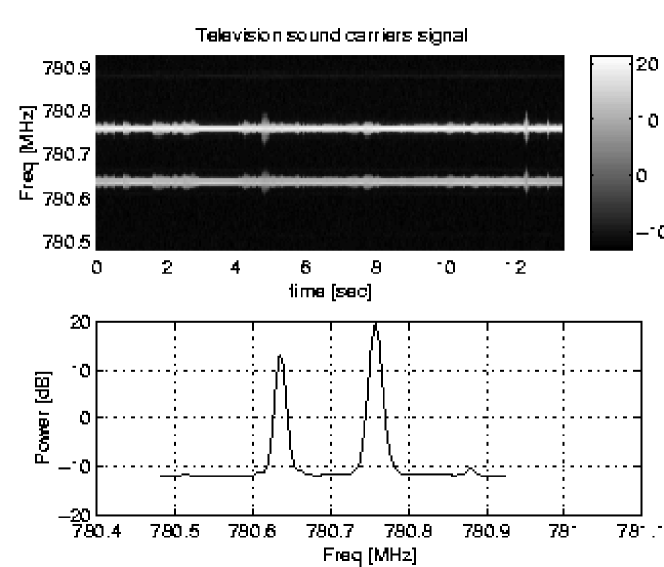
As mentioned before, interference may be continuous or intermittent. A prime example of continuously present interference are television broadcasts. Figure 4 shows a spectrogram centered at 780.75 MHz of the German television transmitter TV Lingen, located at about 80 km southeast of the WSRT. The two strong peaks in the spectrum are the two sound carrier waves. The received power of the TV station is much stronger than the WSRT system noise level, as can be seen from the fact that the baseband filter shape is barely visible.

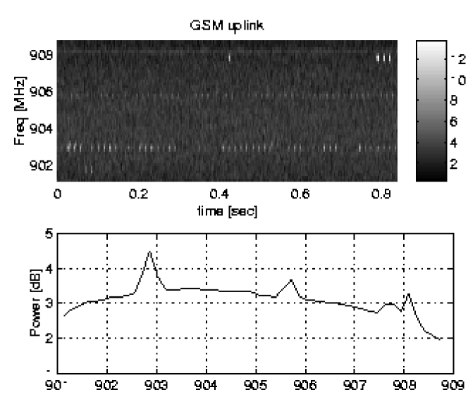
Figure 4 shows the GSM uplink band, which contains the communication of mobile handsets to the base stations. The short white dashes indicate the presence of (weak) interference. At least three channels can be seen at 902.4, 904.4, and 907.2 MHz, although there probably are more active channels at a lower power level. The TDMA time frame format of about 5 ms consisting 8 user slots of 0.577 ms can be recognized. Also visible is a weak continuous transmission at 902 MHz. This is likely to be an interference from the control building or an inter-modulation product.

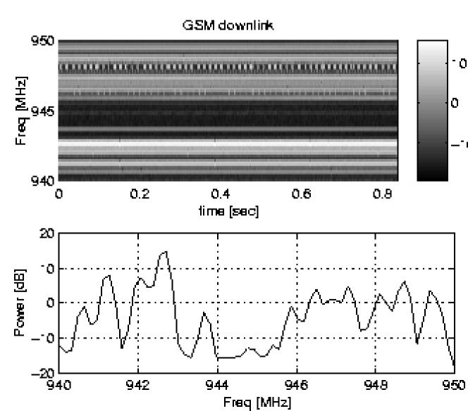
An example of the GSM downlink band (base station to mobiles) is shown in figure 6. Most of the signals are continuous in time, except for a few channels at e.g., 942.0, 942.8, and 949.8 MHz which are time slotted.

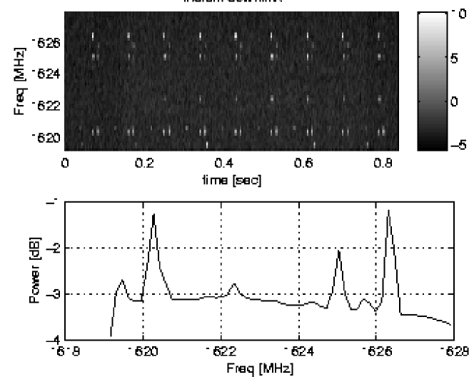
Another interferer which one would like to remove from the observed data is the Iridium transmissions. Figure 6 shows a transmission of the Iridium satellite communication system at 1624 MHz (satellite-satellite communication and/or downlinks). It is clearly intermittent as well.

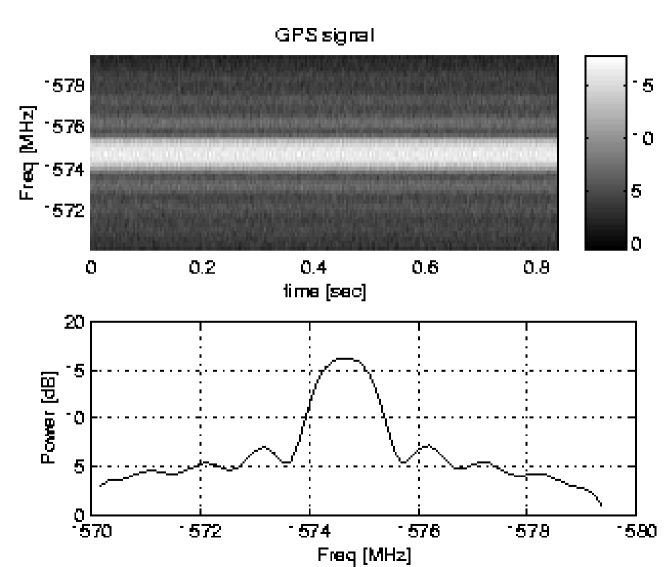
Finally a wideband interferer is the GPS satellite navigation signal. This is a spread spectrum signal occupying a band of $10.23$ MHz. Figure 7 shows a spectrogram of the GPS signal around $1575$ MHz. One can clearly see the superposition of the narrow ($1.023$ MHz) commonly available C/A signal on the wideband ($10.23$ MHz) military P-code signal, resulting in the peak at the center frequencies.

5 INTERFERENCE DETECTION

5.1 Introduction

Ideally, the output of the correlation process produces clean estimates of $\mathbf{A}(t)\mathbf{B}\mathbf{A}(t)^{\raisebox{1.0pt}{$\rm\scriptscriptstyle H$}}$, once every 10 s or so. In principle, we estimate it by

$$\mathbf{\hat{R}}^{10s}_{f}(t)=\frac{1}{N}\sum_{n=0}^{N-1}\mathbf{x}_{f}(t+nT)\mathbf{x}_{f}^{\raisebox{1.0pt}{$\rm\scriptscriptstyle H$}}(t+nT)\,,\qquad NT=10\ \mbox{s}.$$ (8)

As we have seen, these estimates are corrupted by interference and additive system noise, and unknown antenna gains. The objective of interference detection and rejection schemes is to improve the signal to interference and noise ratio (SINR) at the output of the integrators, i.e., at the 10 s level. Interference that is stationary at these time scales or longer can often be treated off-line. In this paper we consider online interference detection and excision schemes, assuming stationarity at millisecond time scales or less.

Many interference detection schemes exist. They differ by the amount of knowledge that we can assume on the interfering signals, e.g., if we know the signal wave form, then the optimal detector has the form of a matched filter. Extensions are possible if the waveform is known up to a few parameters such as amplitude, phase or frequency. However, usually the signal is modulated by a message and hence effectively unknown. There are two classes of detection techniques: more or less deterministic methods that exploit known properties of the signals such as modulation type or certain periodicities, and those based on statistical models with unknown parameters, leading to Generalized Likelihood Ratio Tests (GLRT), a particular example of which is power detection.

In principle, we can say that man-made interference is expected to be statistically different from the astronomical sources. Although this is a very attractive feature, it is not easy to use these properties for detection or excision, since the long averaging periods and the central limit theorem tend to jointly Gaussianize the interferers. For strong narrow-band interferers these methods are expected to give improved suppression at an increased computational expense [8].

Another distinction between interferers and astronomical signals is their spatial signature vectors. Astronomical signals enter through the main lobe of the telescopes and have a very structured (parametrically known) array response (viz. (6)), which is used for imaging. The interferers usually enter through the sidelobes and are in the near field, leading to unstructured $\mathbf{a}$-vectors. Also, their location relative to the array is not correlated with the motion of the earth. It might even remain fixed relative to the array during the complete observation period (e.g., TV transmitters). Since the array tracks a fixed region in the sky which moves as the earth rotates, the directional vector of the interference is typically time varying.

From all possibilities, we consider here two schemes:

• Multichannel interference detection and excision. The interference is detected at short time scales (ms), and contaminated samples are removed from the averaging process in (8). This will work well if the interference is concentrated in frequency and time, as e.g., in the GSM system.

• Spatial filtering. This more ambitious scheme is also suitable for continuously present interference such as TV stations. After detection, we estimate the spatial signature of the interferer and project out that dimension or otherwise subtract the signal coming from that direction.

For the purpose of power detection schemes, it is sufficient to look at (short-term) correlation matrices based on measurement data in a window of length $MT$, with $MT\approx 10\ \mbox{ms}$:

$$\mathbf{\hat{R}}_{k}=\frac{1}{M}\sum_{m=0}^{M-1}\mathbf{x}_{f}(t_{k}+mT)\mathbf{x}_{f}^{\raisebox{1.0pt}{$\rm\scriptscriptstyle H$}}(t_{k}+mT)\,,\qquad t_{k}=0,\;MT,\;2MT,\;\cdots\,.$$

If an interferer is detected in this analysis window, it is discarded, otherwise the data is accepted and the correlation matrix is used in the formation of a clean estimate of $\mathbf{\hat{R}}^{10s}_{f}(t)$, as in figure 2. Obviously, many variations are possible, such as sliding window techniques, or discarding neighbors of contaminated samples as well (perhaps both in time and frequency).

In this section we propose sub-band detection methods based on $\mathbf{\hat{R}}_{k}$ and analyze their performance. Spatial filtering is discussed in section 6. Throughout the section, we will drop the subscript $k$ and write $\mathbf{R}$ and $\mathbf{\hat{R}}$ for simplicity.

5.2 Single channel spectral detector

Detection theory is based on hypothesis testing. We test $\mathcal{H}_{0}$: there is no interference, versus $\mathcal{H}_{1}$: there is at least one interferer in this band. The implementation of this test depends on the model that we pose for the interferer. We will first discuss some particularly simple cases which will allow analysis.

Thus let us consider the single-channel case first. We assume that there is at most a single interferer, where the interfering signal is i.i.d. Gaussian noise with unknown power $\sigma_{s}^{2}$. The background noise is white Gaussian with known power $\sigma^{2}$.

Without interferer, the observed data samples $x_{m}\equiv x(t_{m})$ are complex normal ($\mathcal{C}\mathcal{N}$) distributed, with zero mean and variance $\sigma^{2}$. With an interferer, this distribution is still complex normal, but with variance $\sigma_{s}^{2}+\sigma^{2}$. Thus, we test the hypothesis

$$\begin{array}[]{ll}\mathcal{H}_{0}:&x_{m}\;\sim\;\mathcal{C}\mathcal{N}(0,\,\sigma^{2})\\ \mathcal{H}_{1}:&x_{m}\;\sim\;\mathcal{C}\mathcal{N}(0,\,\sigma_{s}^{2}+\sigma^{2})\,,\qquad m=0,\cdots,M-1\,.\end{array}$$ (9)

We assume that we have available $M$ samples $\{x_{m}\}$, collected in a vector $\mathbf{x}=[x_{1}\,,\cdots\,,x_{M}]$.

This is a rather standard problem in detection theory (see [5] for an introduction). A Neyman-Pearson detector selects $\mathcal{H}_{1}$ if the likelihood ratio,

$$L(\mathbf{x})=\frac{p(\mathbf{x};\mathcal{H}_{1})}{p(\mathbf{x};\mathcal{H}_{0})}\,,$$

exceeds a threshold, where $p(\mathbf{x};\mathcal{H})$ denotes the probability density function of $\mathbf{x}$ under the hypothesis $\mathcal{H}$. It is known that this leads to an optimal probability of detection, given a certain probability of false alarm (detecting an interferer when there is none). In our case, based on the model (9), the Neyman-Pearson detector simplifies to comparing the total received power to a threshold $\gamma$, deciding $\mathcal{H}_{1}$ if the test statistic

$$T(\mathbf{x}):=\frac{1}{\sigma^{2}}\sum_{m=0}^{M-1}|x_{m}|^{2}\quad>\quad\gamma\,.$$

Under the above assumptions we can obtain closed form expressions for the probability of false alarm and the probability of detection. For this, recall that the sum of squares of $M$ real i.i.d. zero-mean unit-variance Gaussian random variables has a chi-square ($\chi^{2}$) distribution with $M$ degrees of freedom. Since we have complex samples, $T(\mathbf{x})$ is the sum-square of $2M$ real variables. Under $\mathcal{H}_{0}$, these have a variance $\frac{1}{2}$, hence the probability of false alarm is given by

$$P_{FA}\;:=\;P\left\{T(\mathbf{x})>\gamma\;;\;\mathcal{H}_{0}\right\}\quad=\quad Q_{\chi^{2}_{2M}}(2\gamma)$$

where $Q_{\chi^{2}_{2M}}(\gamma)$ is the tail probability of a $\chi^{2}$ random variable with ${2M}$ degrees of freedom. It has a closed-form expression (cf. [5]):

$$Q_{\chi^{2}_{2M}}(2\gamma)\;=\;e^{-\gamma}\sum_{k=0}^{M-1}\frac{\gamma^{k}}{k!}\,.$$

Its inverse is known in terms of the inverse Gamma-function, and allows to select $\gamma$ to obtain a desired level of false alarm. Similarly, the probability of detection of an interference at this threshold $\gamma$ is given by

$$\begin{array}[]{lcl}P_{D}&:=&P\{T(\mathbf{x})>\gamma\;;\;\mathcal{H}_{1}\}\\ &=&P\{\frac{1}{\sigma^{2}}\sum_{m=1}^{M}|x_{m}|^{2}>\gamma\;;\;\mathcal{H}_{1}\}\\ &=&\displaystyle P\left\{\frac{2}{\sigma^{2}+\sigma_{s}^{2}}\sum_{m=1}^{M}|x_{m}|^{2}>\frac{2\gamma}{1+\sigma_{s}^{2}/\sigma^{2}}\;;\;\mathcal{H}_{1}\right\}\\ &=&Q_{\chi^{2}_{2M}}(\frac{2\gamma}{1+\mathrm{INR}})\end{array}$$ (10)

where $\mathrm{INR}=\frac{\sigma_{s}^{2}}{\sigma^{2}}$ is the interference-to-noise ratio.

5.3 Multichannel detector with known spatial signature

A significant performance improvement is possible with a multichannel detector. To illustrate this, we assume again the simple case with at most a single narrow-band Gaussian interferer, with known spatial signature vector $\mathbf{a}$ in white Gaussian noise. The source power of the interference is denoted by $\sigma_{s}^{2}$; to normalize the receiver gain we set $\|\mathbf{a}\|^{2}:=\mathbf{a}^{\raisebox{1.0pt}{$\rm\scriptscriptstyle H$}}\mathbf{a}=p$, where $p$ is the number of channels. Without interference, the data vectors $\mathbf{x}_{m}$ are complex normal distributed with zero mean and covariance matrix $\sigma^{2}\mathbf{I}$. With a single interferer, the covariance matrix becomes $\mathbf{R}={\rm E}\{\mathbf{x}_{m}\mathbf{x}_{m}^{\raisebox{1.0pt}{$\rm\scriptscriptstyle H$}}\}=\sigma_{s}^{2}\mathbf{a}\mathbf{a}^{\raisebox{1.0pt}{$\rm\scriptscriptstyle H$}}+\sigma^{2}\mathbf{I}$. Thus,

$$\begin{array}[]{ll}\mathcal{H}_{0}:&\mathbf{x}_{m}\sim\mathcal{C}\mathcal{N}(0,\sigma^{2}\mathbf{I})\\ \mathcal{H}_{1}:&\mathbf{x}_{m}\sim\mathcal{C}\mathcal{N}(0,\sigma_{s}^{2}\mathbf{a}\mathbf{a}^{\raisebox{1.0pt}{$\rm\scriptscriptstyle H$}}+\sigma^{2}\mathbf{I})\,,\qquad m=0,\cdots,M-1\,.\end{array}$$

The Neyman-Pearson detector based on the data matrix $\mathbf{X}=[\mathbf{x}_{1}\,,\cdots,\,\mathbf{x}_{M}]$ considers the estimated data covariance matrix

$$\mathbf{\hat{R}}=\frac{1}{M}\sum_{m=0}^{M-1}\mathbf{x}_{m}\mathbf{x}_{m}^{\raisebox{1.0pt}{$\rm\scriptscriptstyle H$}}$$

and is given by [5]

$$T(\mathbf{X})\quad:=\quad\frac{1}{\sigma^{2}/M}\,\frac{\mathbf{a}^{\raisebox{1.0pt}{$\rm\scriptscriptstyle H$}}{\mathbf{\hat{R}}}\mathbf{a}}{\mathbf{a}^{\raisebox{1.0pt}{$\rm\scriptscriptstyle H$}}\mathbf{a}}\qquad\overset{\mathcal{H}_{1}}{\underset{\mathcal{H}_{0}}{\gtrless}}\quad\gamma\,.$$

This test is recognized as a matched spatial filter detector; essentially we compare the received energy in the direction $\mathbf{a}$ of the interferer to $\sigma^{2}$. If we define $y_{m}$ to be the output of the matched beamformer in the direction of $\mathbf{x}_{m}$,

$$y_{m}=\frac{\mathbf{a}^{\raisebox{1.0pt}{$\rm\scriptscriptstyle H$}}}{\|\mathbf{a}\|}\mathbf{x}_{m}$$

then

$$\begin{array}[]{ll}\mathcal{H}_{0}:&y_{m}\sim\mathcal{C}\mathcal{N}(0,\sigma^{2})\\ \mathcal{H}_{1}:&y_{m}\sim\mathcal{C}\mathcal{N}(0,p\sigma_{s}^{2}+\sigma^{2})\,,\qquad m=0,\cdots,M-1\,.\end{array}$$

and it is seen that taking the same threshold as in the single channel case will provide the same false alarm probability as before:

$$P_{FA}\;=\;P\left\{T(\mathbf{X})>\gamma;\;\mathcal{H}_{0}\right\}\;=\;Q_{\chi^{2}_{2M}}(2\gamma)\,.$$

However, the probability of detection is now given by

$$P_{D}=P\left\{T(\mathbf{X})>\gamma;\;\mathcal{H}_{1}\right\}\;=\;Q_{\chi^{2}_{2M}}(\frac{2\gamma}{1+p\,\mathrm{INR}})\,.$$

Figure 8 presents the probabilities of detection as a function of interference to noise ratio for a single and for $p=14$ channels. We have selected a threshold such that $P_{FA}=5\%$, which means that without interference, we will throw away 5% of the data. We can clearly see that the probability of detection is greatly improved by moving to the multichannel case. The improvement is equal to the array gain, $10\log(p)=11.5$ dB.

5.4 Single TDMA interferer with known spatial signature

Let us now consider a TDMA signal: an interferer which is periodically active in a fraction $\beta$ of the time (see figure 9). Here, $0<\beta<1$ is known as the duty cycle of the periodic signal. Assume that the interferer is present in the selected frequency band and that the duration of the slot in which the interferer is active is equal to $\alpha M$ samples ${\mathbf{x}}_{m}$, where we take $\alpha>1$. Let as before $\sigma_{s}^{2}$ denote the power of a single sample of the interferer when it is present.

Since the interfering slots need not be synchronized to the analysis window, a single interfering slot will give rise to two analysis windows in which the interferer is partially present, and possibly one or more analysis windows in which the interferer is present in all the samples. Since the interferer is time-slotted with duty cycle $\beta$, there will also be windows that contain no interference.

The corresponding probability density $p(I)$ of having a certain average interference power $I$ per sample in an arbitrary analysis window of length $M$ can be computed in closed form, as

$$p(I)=\left\{\begin{array}[]{ll}(1-\displaystyle\frac{\alpha+1}{\alpha}\beta)\,\delta(I)\,,&I=0\\[8.61108pt] \displaystyle\frac{1}{I_{max}}\displaystyle\frac{2}{\alpha}\beta\,,&0<I<I_{max}\\[8.61108pt] \displaystyle\frac{\alpha-1}{\alpha}\beta\,\delta(I-I_{max})\,,&I=I_{max}\,.\end{array}\right.$$

It is plotted in figure 9, where the vertical arrows indicate the unit impulse function $\delta(\,\cdot\,)$. For example, for an interferer of strength $\sigma_{s}^{2}$ per sample when it is on, the maximal average interference power per sample is obviously $\sigma_{s}^{2}$, when all samples are contaminated. The probability of this is $(\alpha-1)/\alpha\,\beta$. Power densities less than $\sigma_{s}^{2}$ occur with a uniform distribution for analysis windows that are only partly corrupted, at the edges of the interference slot.

We can define

• the average interference power per sample before detection:

  $$I_{eff}\;=\;\int\,I\,p(I)\,dI\;=\;\beta\,\sigma_{s}^{2}\,,$$

• the average interference power per sample after detection and blanking:

  $$I_{res}\;=\;\int\,I\,(1-P_{D}(I))\,p(I)\,dI\,,$$

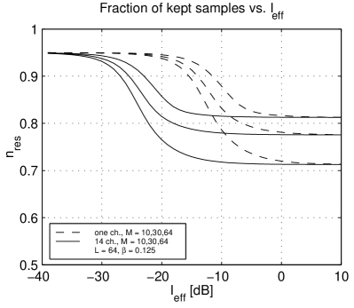
• the fraction of number of samples kept after detection and blanking:

  $$n_{res}\;=\;\int\,(1-P_{D}(I))\,p(I)\,dI\,.$$

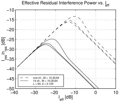
Figure 10 shows the dependence of the residual INR as a function of $M$ (the number of samples in an analysis block), for an interferer of length $L=64$ sub-band samples, a duty cycle $\beta=1/8$, and a false alarm rate of $5\%$. Obviously, very weak interference is not detected, and in that case we throw away $5\%$ of the data due to the false alarm rate. High interference powers are easily detected, and almost all contaminated analysis windows will be detected and blanked. Only the tails of an interfering slot might be missed, so that there is still some interference remaining after detection. The worst case occurs for interference that is not strong enough to be detected all the time, but not weak enough to be harmless.

Several other interesting facts can be seen in these figures. The most important is the large performance gain in the multichannel approach, as compared to a single channel. As seen in figure 8, the effect of using an array is to shift the graphs of probability of detection to the left by the array gain, e.g., for the 14-channel detector the graph is shifted by $11.5$ dB. Hence, we require 11.5 dB less interference power in order to detect it. However, the effective gain is given by the vertical distance between the graphs: this shows the amount of interference suppression for a given interference power. In figure 10 the suppression can be approximately $21$ dB larger than that of the single antenna case.

A second interesting phenomenon is the fact that the interference suppression is almost the same for a large range of analysis windows $M$. Thus, we would take this window rather small, so that the residual number of samples is larger. This effect is mainly due to the fact that the case of partial blocks with weaker power is less frequent as the analysis block becomes shorter. Further study of this model appeared in [9].

5.5 Eigenvalue analysis

So far, we have looked at the detection problem from a rather idealistic viewpoint: at most 1 interferer, and a known spatial signature. The reason was that for this case, we could derive optimal detectors with closed-form expressions for the performance. We will now discuss an extension to more practical situations.

Our goal is the detection of the presence of an interferer from observed correlation data. As a start, let us first consider the covariance matrix due to $q$ interferers and no noise,

$$\mathbf{R}=\mathbf{A}_{s}\mathbf{R}_{s}\mathbf{A}_{s}^{\raisebox{1.0pt}{$\rm\scriptscriptstyle H$}}$$

where $\mathbf{R}$ has size $p\times p$, $\mathbf{A}_{s}$ has size $p\times q$ and $\mathbf{R}_{s}$ has size $q\times q$. For a low number of interferers $q$, this brings us to familiar grounds in array signal processing, as it admits analysis by subspace-based techniques. We give a brief introduction here; see [7] for an overview and references.

If $q<p$, then the rank of $\mathbf{R}$ is $q$ since $\mathbf{A}_{s}$ has only $q$ columns. Thus, we can estimate the number of narrow-band interferers from a rank analysis. This is also seen from an eigenvalue analysis: let

$$\mathbf{R}=\mathbf{U}\mbox{$\mbox{\boldmath$\Lambda$}$}\mathbf{U}^{\raisebox{1.0pt}{$\rm\scriptscriptstyle H$}}$$

be an eigenvalue decomposition of $\mathbf{R}$, where the $p\times p$ matrix $\mathbf{U}$ is unitary ($\mathbf{U}\mathbf{U}^{\raisebox{1.0pt}{$\rm\scriptscriptstyle H$}}=\mathbf{I}$, $\mathbf{U}^{\raisebox{1.0pt}{$\rm\scriptscriptstyle H$}}\mathbf{U}=\mathbf{I}$) and contains the eigenvectors, and the $p\times p$ diagonal matrix $\Lambda$ contains the corresponding eigenvalues in non increasing order ($\lambda_{1}\geq\lambda_{2}\geq\cdots\geq\lambda_{p}\geq 0$). Since the rank is $q$, there are only $q$ nonzero eigenvalues. We can collect these in a $q\times q$ diagonal matrix $\mbox{$\mbox{\boldmath$\Lambda$}$}_{s}$, and the corresponding eigenvectors in a $p\times q$ matrix $\mathbf{U}_{s}$, so that

$$\mathbf{R}=\mathbf{U}_{s}\mbox{$\mbox{\boldmath$\Lambda$}$}_{s}\mathbf{U}_{s}^{\raisebox{1.0pt}{$\rm\scriptscriptstyle H$}}\,.$$ (11)

The remaining $p-q$ eigenvectors from $\mathbf{U}$ can be collected in a matrix $\mathbf{U}_{n}$, and they are orthogonal to $\mathbf{U}_{s}$ since $\mathbf{U}=[\mathbf{U}_{s}\;\;\mathbf{U}_{n}]$ is unitary. The subspace spanned by the columns of $\mathbf{U}_{s}$ is called the signal subspace, the orthogonal complement spanned by the columns of $\mathbf{U}_{n}$ is known as the noise subspace (although this is a misnomer). Thus, in the noise-free case,

$$\mathbf{R}=\mathbf{U}\mbox{$\mbox{\boldmath$\Lambda$}$}\mathbf{U}^{\raisebox{1.0pt}{$\rm\scriptscriptstyle H$}}=[\mathbf{U}_{s}\quad\mathbf{U}_{n}]\left[\begin{array}[]{c|c}\mbox{$\mbox{\boldmath$\Lambda$}$}_{s}&0\\ \hline\cr 0&0\end{array}\right]\left[\begin{array}[]{c}\mathbf{U}_{s}^{\raisebox{1.0pt}{$\rm\scriptscriptstyle H$}}\\ \mathbf{U}_{n}^{\raisebox{1.0pt}{$\rm\scriptscriptstyle H$}}\end{array}\right]$$

In the presence of white noise,

$$\mathbf{R}\;=\;\mathbf{A}_{s}\mathbf{R}_{s}\mathbf{A}_{s}^{\raisebox{1.0pt}{$\rm\scriptscriptstyle H$}}+\sigma^{2}\mathbf{I}_{p}\,.$$

($\mathbf{I}_{p}$ denotes a $p\times p$ identity matrix.) In this case, $\mathbf{R}$ is full rank: its rank is always $p$. However, we can still detect the number of interferers by looking at the eigenvalues of $\mathbf{R}$. Indeed, the eigenvalue decomposition is derived as (expressed in terms of the previous decomposition (11) and using the fact that $\mathbf{U}=[\mathbf{U}_{s}\quad\mathbf{U}_{n}]$ is unitary: $\mathbf{U}_{s}\mathbf{U}_{s}^{\raisebox{1.0pt}{$\rm\scriptscriptstyle H$}}+\mathbf{U}_{n}\mathbf{U}_{n}^{\raisebox{1.0pt}{$\rm\scriptscriptstyle H$}}=\mathbf{I}_{p}$)

$$\begin{array}[]{lcl}\mathbf{R}&=&\mathbf{A}_{s}\mathbf{R}_{s}\mathbf{A}_{s}^{\raisebox{1.0pt}{$\rm\scriptscriptstyle H$}}+\sigma^{2}\mathbf{I}_{p}\\ &=&\mathbf{U}_{s}\mbox{$\mbox{\boldmath$\Lambda$}$}_{s}\mathbf{U}_{s}^{\raisebox{1.0pt}{$\rm\scriptscriptstyle H$}}+\sigma^{2}(\mathbf{U}_{s}\mathbf{U}_{s}^{\raisebox{1.0pt}{$\rm\scriptscriptstyle H$}}+\mathbf{U}_{n}\mathbf{U}_{n}^{\raisebox{1.0pt}{$\rm\scriptscriptstyle H$}})\\ &=&\mathbf{U}_{s}(\mbox{$\mbox{\boldmath$\Lambda$}$}_{s}+\sigma^{2}\mathbf{I}_{q})\mathbf{U}_{s}^{\raisebox{1.0pt}{$\rm\scriptscriptstyle H$}}+\mathbf{U}_{n}(\sigma^{2}\mathbf{I}_{p-q})\mathbf{U}_{n}^{\raisebox{1.0pt}{$\rm\scriptscriptstyle H$}}\\ &=&[\mathbf{U}_{s}\quad\mathbf{U}_{n}]\left[\begin{array}[]{c|c}\mbox{$\mbox{\boldmath$\Lambda$}$}_{s}+\sigma^{2}\mathbf{I}_{q}&0\\ \hline\cr 0&\sigma^{2}\mathbf{I}_{p-q}\end{array}\right]\left[\begin{array}[]{c}\mathbf{U}_{s}^{\raisebox{1.0pt}{$\rm\scriptscriptstyle H$}}\\ \mathbf{U}_{n}^{\raisebox{1.0pt}{$\rm\scriptscriptstyle H$}}\end{array}\right]\\ &=:&\mathbf{U}\mbox{$\mbox{\boldmath$\Lambda$}$}\mathbf{U}^{\raisebox{1.0pt}{$\rm\scriptscriptstyle H$}}\end{array}$$ (12)

hence $\mathbf{R}$ has $p-q$ eigenvalues equal to $\sigma^{2}$, and $q$ that are larger than $\sigma^{2}$. Thus, we can detect the number of interferers $q$ by comparing the eigenvalues of $\mathbf{R}$ to a threshold defined by $\sigma^{2}$.

A physical interpretation of the eigenvalue decomposition can be as follows. The eigenvectors give an orthogonal set of “directions” (spatial signatures) present in the covariance matrix, sorted in decreasing order of dominance. The eigenvalues give the power of the signal coming from the corresponding directions, or the power of the output of a beamformer matched to that direction. Indeed, let the $i$’th eigenvector be $\mathbf{u}_{i}$, then this output power will be

$$\mathbf{u}_{i}^{\raisebox{1.0pt}{$\rm\scriptscriptstyle H$}}\mathbf{R}\mathbf{u}_{i}=\lambda_{i}\,.$$

The first eigenvector, $\mathbf{u}_{1}$, is always pointing in the direction from which most energy is coming. The second one, $\mathbf{u}_{2}$, points in a direction orthogonal to $\mathbf{u}_{1}$ from which most of the remaining energy is coming, etcetera.

If there is no interference and only noise, then there is no dominant direction, and all eigenvalues are equal to the noise power. If there is a single interferer with power $\sigma_{s}^{2}$ and spatial signature $\mathbf{a}$, normalized to $\|\mathbf{a}\|^{2}=p$, then the covariance matrix is $\mathbf{R}=\sigma_{s}^{2}\mathbf{a}\mathbf{a}^{\raisebox{1.0pt}{$\rm\scriptscriptstyle H$}}+\sigma^{2}\mathbf{I}$. It follows from the previous that there is only one eigenvalue larger than $\sigma^{2}$. The corresponding eigenvector is $\mathbf{u}_{1}=\mathbf{a}\frac{1}{\|\mathbf{a}\|}$, and is in the direction of $\mathbf{a}$. The power coming from that direction is

$$\lambda_{1}=\mathbf{u}_{1}^{\raisebox{1.0pt}{$\rm\scriptscriptstyle H$}}\mathbf{R}\mathbf{u}_{1}=p\sigma_{s}^{2}+\sigma^{2}\,.$$

Since there is only one interferer, the power coming from any other direction orthogonal to $\mathbf{u}_{1}$ is $\sigma^{2}$, the noise power. Note the connection with the test statistic of the previous section, where we assumed that $\mathbf{a}$ is known. Since $\mathbf{u}_{1}=\mathbf{a}\frac{1}{\|\mathbf{a}\|}$,

$$\frac{\mathbf{a}^{\raisebox{1.0pt}{$\rm\scriptscriptstyle H$}}\mathbf{R}\mathbf{a}}{\mathbf{a}^{\raisebox{1.0pt}{$\rm\scriptscriptstyle H$}}\mathbf{a}}=\frac{\mathbf{u}_{1}^{\raisebox{1.0pt}{$\rm\scriptscriptstyle H$}}\mathbf{R}\mathbf{u}_{1}}{\mathbf{u}_{1}^{\raisebox{1.0pt}{$\rm\scriptscriptstyle H$}}\mathbf{u}_{1}}=\lambda_{1}\,.$$

Thus, the test statistic of the previous section reduces to testing the dominant eigenvalue of $\mathbf{R}$, and knowledge of $\mathbf{a}$ is in fact not needed.

With more than one interferer, this generalizes. Suppose there are two interferers with powers $\sigma_{1}$ and $\sigma_{2}$, and spatial signatures $\mathbf{a}_{1}$ and $\mathbf{a}_{2}$. If the spatial signatures are orthogonal, $\mathbf{a}_{1}^{\raisebox{1.0pt}{$\rm\scriptscriptstyle H$}}\mathbf{a}_{2}=0$, then $\mathbf{u}_{1}$ will be in the direction of the strongest interferer, number 1 say, and $\lambda_{1}$ will be the corresponding power, $\lambda_{1}=p\sigma_{1}^{2}+\sigma^{2}$. Similarly, $\lambda_{2}=p\sigma_{2}^{2}+\sigma^{2}$.

In general, the spatial signatures are not orthogonal to each other. In that case, $\mathbf{u}_{1}$ will point into the direction that is common to both $\mathbf{a}_{1}$ and $\mathbf{a}_{2}$, and $\mathbf{u}_{2}$ will point in the remaining direction orthogonal to $\mathbf{u}_{1}$. The power $\lambda_{1}$ coming from direction $\mathbf{u}_{1}$ will be larger than before because it combines power from both interferers, whereas $\lambda_{2}$ will be smaller.

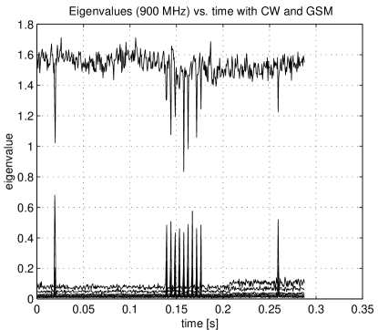
The covariance matrix eigenvalue structure can be nicely illustrated on data collected at the WSRT. We selected a narrow band slice (52 kHz) of a GSM uplink data file, around $900$ MHz. In this subband we have two interfering signals: a continuous narrow band CW signal which leaked in from a local oscillator, and a weak GSM signal. From this data we computed a sequence of short term cross spectral matrices $\hat{\mathbf{R}}^{0.5ms}_{k}$ based on $0.5$ ms averages. Figure 11 shows the time evolution of the eigenvalues of these matrices. The largest eigenvalue is due to the CW signal and is always present. The GSM interference is intermittent: at time intervals where it is present the number of large eigenvalues increases to two. The remaining eigenvalues are at the noise floor, $\sigma^{2}$. The small step in the noise floor after $0.2$ s is due to a periodically switched calibration noise source at the input of the telescope front ends.

The eigenvalue decomposition (12) shows more than just the number of interferers. Indeed, the columns of $\mathbf{U}_{s}$ span the same subspace as the columns of $\mathbf{A}_{s}$. This is clear in the noise-free case (11), but the decomposition (12) shows that the eigenvectors contained in $\mathbf{U}_{s}$ and $\mathbf{U}_{n}$ respectively are the same as in the noise-free case. Thus,

$$\mathrm{span}(\mathbf{U}_{s})=\mathrm{span}(\mathbf{A}_{s})\,,\qquad\mathbf{U}_{n}^{\raisebox{1.0pt}{$\rm\scriptscriptstyle H$}}\mathbf{A}_{s}=0\,.$$ (13)

Given a correlation matrix $\mathbf{\hat{R}}$ estimated from the data, we compute its eigenvalue decomposition. From this we can detect the rank $q$ from the number of eigenvalues larger than $\sigma^{2}$, and we can determine $\mathbf{U}_{s}$ and hence the subspace spanned by the columns of $\mathbf{A}_{s}$. Although we cannot directly identify each individual column of $\mathbf{A}_{s}$, its subspace estimate can nonetheless be used to filter out the interference — such spatial filtering algorithms are discussed in section 6. Note that it is crucial that the noise is spatially white. For colored noise, an extension (whitening) is possible but we have to know the coloring.

5.6 Multichannel detector with unknown spatial signature

In case we only have an estimate $\mathbf{\hat{R}}$ based on a finite amount of samples $M$ and the spatial signature vectors of the interference are unknown, there are no optimal results. The eigenvalue analysis suggested that we should compare the eigenvalues to a threshold defined by $\sigma^{2}$: without interference, all eigenvalues are asymptotically equal to $\sigma^{2}$. We will discuss two detectors, one for the case where $\sigma^{2}$ is known, and another one for which it is unknown.

If the noise power $\sigma^{2}$ is known, we can apply the (generalized) likelihood ratio test (GLRT), which leads to a method due to Box [2] for testing the null hypothesis that $\sigma^{-2}\mathbf{\hat{R}}=\mathbf{I}$ (no interference). The GLRT leads to a test statistic given by

$$T(\mathbf{X})\;:=\;-Mp\log\prod_{i=1}^{p}\frac{\mbox{$\hat{\lambda}$}_{i}}{\sigma^{2}}$$ (14)

where $\mbox{$\hat{\lambda}$}_{i}$ is the $i$-th eigenvalue of $\mathbf{\hat{R}}$, and we detect an interferer if $T(\mathbf{X})>\gamma$. This basically tests if all eigenvalues are equal to $\sigma^{2}$, with a certain confidence. In the no-interference case, one can show that

$$T(\mathbf{X})\quad\sim\quad\chi^{2}_{(p+1)(p-2)}$$

This allows to select the value of $\gamma$ to achieve a desired false alarm rate.

If also the noise power is unknown, we propose to use the Minimum Description Length (MDL) detector [Wax $\&$ Kailath [18]]. In this case, rather than setting a threshold based on the asymptotic distribution of the LRT, we try to find the correct model order which minimizes the description length of the data. The MDL rank estimator is given by

$$\hat{q}=\arg\min_{n}\mathrm{MDL}(n)$$ (15)

where

$$\mathrm{MDL}(n)\;=\;-(p-n)M\log\frac{\left(\prod_{i=n+1}^{p}\mbox{$\hat{\lambda}$}_{i}\right)^{\frac{1}{p-n}}}{\frac{1}{p-n}\sum_{i=n+1}^{p}\mbox{$\hat{\lambda}$}_{i}}\quad+\;\frac{1}{2}n(2p-n+1)\log M$$

and an interference is detected if $\hat{q}\not=0$. The first term basically tests if the geometric mean of the smallest $p-n$ eigenvalues is equal to the arithmetic mean, which is only true if these eigenvalues are equal to each other. (The second term is a correction that grows with the number of unknown parameters to be estimated). Note also that the arithmetic mean of the small eigenvalues is an estimate of the noise variance, so in the case of testing whether $n=0$ or not the first term in the MDL reduces to a sample estimate $T(\mathbf{x})$ of (14). This rank detector is simple to implement since it is independent of the varying SINR in the system. A disadvantage is that the false alarm rate is not known and not fixed.

Finally a simple option which can be used to limit the false alarm rate is to collect a number of processing blocks, sort them according to the value of the statistic $T(\mathbf{x})$, defined in (14) and throw away a given percentage with the highest score. This is conceptually simple but needs more memory available.

Experimental results on multichannel blanking are presented in section 7.

6 SPATIAL FILTERING

Let us now assume that we have obtained a covariance matrix $\mathbf{R}$, which contains the rather weak covariance matrix of the astronomical sources (visibilities) $\mathbf{R}_{v}$, plus white noise. Suppose also that there is an interferer with power $\sigma^{2}_{s}$:

$$\mathbf{R}\;=\;\mathbf{R}_{v}\;+\;\sigma^{2}_{s}\mathbf{a}\mathbf{a}^{\raisebox{1.0pt}{$\rm\scriptscriptstyle H$}}\;+\;\sigma^{2}\mathbf{I}\,.$$

In the previous section, we considered schemes to detect the interferer from the eigenvalues of $\hat{\mathbf{R}}$, a short-term estimate of $\mathbf{R}$. After detection, we proposed to discard $\hat{\mathbf{R}}$ from a longer-term average if it is found to be contaminated, but what if the interferer is present all the time? In that case, it is more suitable to try to suppress its contribution $\sigma^{2}_{s}\mathbf{a}\mathbf{a}^{\raisebox{1.0pt}{$\rm\scriptscriptstyle H$}}$. This leads to spatial filtering techniques.

6.1 Projecting out the interferer

An elementary form of spatial filtering is to null all energy with spatial signature $\mathbf{a}$. To this end, we can introduce the $p\times p$ projection matrix

$$\mathbf{P}_{\mathbf{a}}^{\perp}=\mathbf{I}-\mathbf{a}(\mathbf{a}^{\raisebox{1.0pt}{$\rm\scriptscriptstyle H$}}\mathbf{a})^{-1}\mathbf{a}^{\raisebox{1.0pt}{$\rm\scriptscriptstyle H$}}\,.$$

$\mathbf{P}_{\mathbf{a}}^{\perp}$ is a projection because $\mathbf{P}_{\mathbf{a}}^{\perp}\mathbf{P}_{\mathbf{a}}^{\perp}=\mathbf{P}_{\mathbf{a}}^{\perp}$. It is also easily seen that $\mathbf{P}_{\mathbf{a}}^{\perp}\mathbf{a}={\bf 0}$: this direction is projected out. If we denote by $\mathbf{\tilde{R}}$ the filtered covariance matrix, we obtain

$$\mathbf{\tilde{R}}:=\mathbf{P}^{\perp}_{\mathbf{a}}\mathbf{R}\mathbf{P}^{\perp}_{\mathbf{a}}\;=\;\mathbf{P}^{\perp}_{\mathbf{a}}\mathbf{R}_{v}\mathbf{P}^{\perp}_{\mathbf{a}}\;+\;\sigma^{2}\mathbf{P}^{\perp}_{\mathbf{a}}\,.$$ (16)

Thus, the interference is removed by the projection. At the same time, the visibility matrix is modified by the projections, and the noise is not white anymore, since one dimension is missing. The imaging stage has to be aware of this, which is the topic of [10].

In general, $\mathbf{a}$ is not known. However, note that we do not need $\mathbf{a}$, but only a projection matrix to project it out. Recall from equation (12) the eigenvalue decomposition of $\mathbf{R}$, and in particular the matrix containing an orthonormal basis of the “noise subspace” $\mathbf{U}_{n}$, which is the orthogonal complement of $\mathbf{a}$, with $p-1$ columns. According to (13), $\mathbf{U}_{n}^{\raisebox{1.0pt}{$\rm\scriptscriptstyle H$}}\mathbf{a}=0$. It is now straightforward to show that

$$\mathbf{P}_{\mathbf{a}}^{\perp}=\mathbf{U}_{n}\mathbf{U}_{n}^{\raisebox{1.0pt}{$\rm\scriptscriptstyle H$}}$$ (17)

Indeed, since $\mathbf{U}_{n}^{\raisebox{1.0pt}{$\rm\scriptscriptstyle H$}}\mathbf{U}_{n}=\mathbf{I}_{p-1}$,

$$\mathbf{P}_{\mathbf{a}}^{\perp}\mathbf{P}_{\mathbf{a}}^{\perp}\;=\;\mathbf{U}_{n}\mathbf{U}_{n}^{\raisebox{1.0pt}{$\rm\scriptscriptstyle H$}}\mathbf{U}_{n}\mathbf{U}_{n}^{\raisebox{1.0pt}{$\rm\scriptscriptstyle H$}}\;=\;\mathbf{U}_{n}\mathbf{U}_{n}^{\raisebox{1.0pt}{$\rm\scriptscriptstyle H$}}\;=\;\mathbf{P}_{\mathbf{a}}^{\perp}$$

and

$$\mathbf{P}_{\mathbf{a}}^{\perp}\mathbf{a}\;=\;\mathbf{U}_{n}\mathbf{U}_{n}^{\raisebox{1.0pt}{$\rm\scriptscriptstyle H$}}\mathbf{a}\;=\;{\bf 0}\,.$$

Thus, we can compute the required projection matrix directly from the eigenvalue decomposition of $\mathbf{R}$.

Expression (17) can immediately be generalized to the more general case of $q<p$ interferers and unknown $\mathbf{a}$-vectors. Indeed, in this case, the projection onto the complement of the $\mathbf{A}_{s}$-matrix of the interference is given by

$$\mathbf{P}_{\mathbf{A}_{s}}^{\perp}=\mathbf{I}-\mathbf{A}_{s}(\mathbf{A}_{s}^{\raisebox{1.0pt}{$\rm\scriptscriptstyle H$}}\mathbf{A}_{s})^{-1}\mathbf{A}_{s}^{\raisebox{1.0pt}{$\rm\scriptscriptstyle H$}}=\mathbf{U}_{n}\mathbf{U}_{n}^{\raisebox{1.0pt}{$\rm\scriptscriptstyle H$}}$$

Note that we do not have to know $\mathbf{A}_{s}$: the relevant noise subspace is estimated from the eigenvalue decomposition of $\mathbf{R}$. This hinges upon the fact that the noise covariance is white (in general: known), and the visibility matrix $\mathbf{R}_{v}$ is insignificant at these time scales (otherwise, it might disturb the eigenvalue decomposition).

As an alternative to (16), we can define another filtered covariance matrix

$$\mathbf{\tilde{R}}:=\mathbf{U}_{n}^{\raisebox{1.0pt}{$\rm\scriptscriptstyle H$}}\mathbf{R}\mathbf{U}_{n}\;=\;\mathbf{U}_{n}^{\raisebox{1.0pt}{$\rm\scriptscriptstyle H$}}\mathbf{R}_{v}\mathbf{U}_{n}\;+\;\sigma^{2}\mathbf{I}_{p-q}\,,$$ (18)

where we have used $\mathbf{U}_{n}\perp\mathbf{A}_{s}$ and $\mathbf{U}_{n}^{\raisebox{1.0pt}{$\rm\scriptscriptstyle H$}}\mathbf{U}_{n}=I_{p-q}$. In this case, $\mathbf{\tilde{R}}$ has size $(p-q)\times(p-q)$. Although smaller, this matrix contains the same information as $\mathbf{P}^{\perp}_{\mathbf{a}}\mathbf{R}\mathbf{P}^{\perp}_{\mathbf{a}}$. Besides the dimension reduction, an advantage of this scheme is that the noise term stays white.

6.2 Keeping track of projections

Since the projections alter the visibility data in $\mathbf{R}_{v}$, it is essential, for the purpose of imaging, to store the linear operation represented by the projections. At the same time, it might be necessary to adapt the projection several times per second, since the $\mathbf{a}$-vectors of interferers are time-varying. Hence, in the construction of the 10 s correlation average from short-term projected correlation matrices, we also have to construct the effective linear operation.

Let $\mathbf{R}_{k}$ denote the short-term correlation matrix, where $k=0,1,\cdots,N-1$ is the time index, and $N$ is the number of short-term matrices used in the long-term average. Denote for generality the linear operation representing the projection by $\mathbf{L}_{k}$, where $\mathbf{L}_{k}=(\mathbf{U}_{n})_{k}(\mathbf{U}_{n})_{k}^{\raisebox{1.0pt}{$\rm\scriptscriptstyle H$}}$ in the first filtering scheme (equation (16)), and $\mathbf{L}_{k}=(\mathbf{U}_{n})_{k}^{\raisebox{1.0pt}{$\rm\scriptscriptstyle H$}}$ in the second (equation (18)). Consider now the short-term filtered averages,

$$\mathbf{\tilde{R}}_{k}:=\mathbf{L}_{k}\mathbf{R}_{k}\mathbf{L}_{k}^{\raisebox{1.0pt}{$\rm\scriptscriptstyle H$}}\;=\;\mathbf{L}_{k}\mathbf{R}_{v}\mathbf{L}_{k}^{\raisebox{1.0pt}{$\rm\scriptscriptstyle H$}}\;+\;\sigma^{2}\mathbf{L}_{k}\mathbf{L}_{k}^{\raisebox{1.0pt}{$\rm\scriptscriptstyle H$}}\,,\qquad k=0,1,\cdots,N-1\,.$$

By simply averaging these, the long-term average will be

$$\mathbf{\tilde{R}}^{10s}\;=\;\frac{1}{N}\sum_{k=0}^{N-1}\mathbf{\tilde{R}}_{k}\;=\;\frac{1}{N}\sum_{k=0}^{N-1}\mathbf{L}_{k}\mathbf{R}_{k}\mathbf{L}_{k}^{\raisebox{1.0pt}{$\rm\scriptscriptstyle H$}}\,.$$

The $\mathbf{L}_{k}$ appear here at both sides of $\mathbf{R}_{k}$. To move them to one side, we make use of the general expression

$$\mathrm{vec}(\mathbf{A}\mathbf{B}\mathbf{C})=(\mathbf{C}^{\raisebox{1.2pt}{$\rm\scriptstyle T$}}\otimes\mathbf{A})\mathrm{vec}(\mathbf{B})$$

where $\otimes$ denotes a Kronecker product, and $\mathrm{vec}(\cdot)$ the column-wise stacking of a matrix into a vector,

$$\mathbf{A}\otimes\mathbf{B}:=\left[\begin{array}[]{ccc}a_{11}\mathbf{B}&a_{12}\mathbf{B}&\cdots\\ a_{21}\mathbf{B}&a_{22}\mathbf{B}&\cdots\\ \vdots&&\ddots\end{array}\right]$$

$$\mathbf{A}=[\mathbf{a}_{1}\quad\mathbf{a}_{2}\quad\cdots]\quad\Rightarrow\quad\mathrm{vec}(\mathbf{A}):=\left[\begin{array}[]{c}\mathbf{a}_{1}\\ \mathbf{a}_{2}\\ \vdots\end{array}\right]$$

In this case, we obtain

$$\begin{array}[]{lcl}\mathrm{vec}(\mathbf{\tilde{R}}^{10s})&=&\frac{1}{N}\sum\left[(\mathbf{\bar{L}}_{k}\otimes\mathbf{L}_{k})\mathrm{vec}(\mathbf{R}_{k})\right]\\ &=&\left[\frac{1}{N}\sum\mathbf{\bar{L}}_{k}\otimes\mathbf{L}_{k}\right]\mathrm{vec}(\mathbf{R}_{v})\;+\;\sigma^{2}\left[\frac{1}{N}\sum\mathbf{\bar{L}}_{k}\otimes\mathbf{L}_{k}\right]\mathrm{vec}(\mathbf{I}_{p})\\ &=&\mathbf{C}\mathrm{vec}(\mathbf{R}_{v})\;+\;\sigma^{2}\mathbf{C}\mathrm{vec}(\mathbf{I}_{p})\end{array}$$

where

$$\mathbf{C}\;:=\;\frac{1}{N}\sum_{k=0}^{N-1}\mathbf{\bar{L}}_{k}\otimes\mathbf{L}_{k}$$

and the overbar denotes complex conjugation. $\mathbf{C}$ is the effective linear mapping of entries of $\mathbf{R}_{v}$ to entries of $\mathbf{\tilde{R}}^{10s}$. For the imaging step, we have to know how $\mathbf{\tilde{R}}^{10s}$ depends on $\mathbf{R}_{v}$. Thus, we have to construct and store $\mathbf{C}$ along with $\mathbf{\tilde{R}}^{10s}$. Unfortunately, it is a rather large matrix: $p^{2}\times p^{2}$ in the first filtering scheme, and $(p-q)^{2}\times p^{2}$ in the second. Another problem for imaging might be that the noise contribution on $\mathbf{\tilde{R}}^{10s}$ is no longer white, but determined by $\mathbf{C}$. Two possible remedies are

• Assume that the $\mathbf{a}$-vectors were sufficiently variable over the time interval. In that case, $\mathbf{C}$ is likely to be of full rank and thus invertible, and we can construct

  $$\mathbf{C}^{-1}\mathrm{vec}(\mathbf{\tilde{R}}^{10s})=\mathrm{vec}(\mathbf{R}_{v})\;+\;\sigma^{2}\mathrm{vec}(\mathbf{I}_{p})\,.$$

  By unstacking the result, we recover our interference-free model $\mathbf{R}_{v}+\sigma^{2}\mathbf{I}$. However, the inversion of $\mathbf{C}$ might be a formidable, and numerically dubious, task.

• If we take $\mathbf{L}_{k}=(\mathbf{U}_{n})_{k}^{\raisebox{1.0pt}{$\rm\scriptscriptstyle H$}}$ as in (18), then the noise contribution on each $\mathbf{\tilde{R}}_{k}$ is white. We can average the $\mathbf{\tilde{R}}_{k}$ if they have the same dimension, i.e., $p-q$ where the number of interferers $q$ is constant over the interval. In that case,

  $$\sigma^{2}\frac{1}{N}\sum_{n=0}^{N-1}(\mathbf{U}_{n})_{k}^{\raisebox{1.0pt}{$\rm\scriptscriptstyle H$}}(\mathbf{U}_{n})_{k}\;=\;\sigma^{2}\mathbf{I}_{p-q}$$

  so that the noise contribution on $\mathbf{\tilde{R}}^{10s}$ is white. Note that no inversion is necessary.

If we do not invert $\mathbf{C}$ then the observed visibilities $V(u_{ij},v_{ij})$ in the matrix $\mathbf{R}_{v}$ are modified by some (known) linear combination. This has implications for the synthesis imaging step. The usual construction of an image using inverse Fourier transformation (based on (3)) now gives rise to a point-source image convolved with a space-varying point spread function (“dirty beam”). Since the point spread function is known at every location in the image, it is still possible to correct for it using an extension of the usual CLEAN deconvolution algorithm. Details are in [10].

Since $\mathbf{C}$ is a factor $p^{2}$ larger than $\mathbf{\tilde{R}}^{10s}$, it might in fact be more efficient to store the sequence of spatial filters $\mathbf{L}_{k}$. This is the case if $\mathbf{L}_{k}$ is to be updated at time scales of $10~{}\mbox{s}/p^{2}=50$ ms or longer.

6.3 Other spatial filtering possibilities

Without going into too much detail, we mention a few other possibilities for spatial filtering and interference cancellation. Suppose there is a single interferer,

$$\mathbf{R}=\mathbf{R}_{v}+\sigma_{s}^{2}\mathbf{a}\mathbf{a}^{\raisebox{1.0pt}{$\rm\scriptscriptstyle H$}}+\sigma^{2}\mathbf{I}\,.$$

• Subtraction. With an estimate of $\mathbf{a}$ and $\sigma_{s}^{2}$, we can try to subtract it from the covariance data:

  $$\mathbf{\tilde{R}}=\mathbf{R}-\hat{\sigma}_{s}^{2}\mathbf{\hat{a}}\mathbf{\hat{a}}^{\raisebox{1.0pt}{$\rm\scriptscriptstyle H$}}\,.$$ (19)

  Without other knowledge, the best estimate of $\mathbf{a}$ is the dominant eigenvector, $\mathbf{u}_{1}$, of $\mathbf{R}$, and likewise the best estimate of $\sigma_{s}^{2}$ is $\lambda_{1}-\sigma^{2}$. Since both of these are derived from $\mathbf{R}$, it turns out to be not too different from the projection scheme. Indeed, if we look at

  $$(\mathbf{I}-\alpha\mathbf{u}_{1}\mathbf{u}_{1}^{\raisebox{1.0pt}{$\rm\scriptscriptstyle H$}})\mathbf{R}(\mathbf{I}-\alpha\mathbf{u}_{1}\mathbf{u}_{1}^{\raisebox{1.0pt}{$\rm\scriptscriptstyle H$}})\;=\;\mathbf{R}-\mathbf{u}_{1}\mathbf{u}_{1}^{\raisebox{1.0pt}{$\rm\scriptscriptstyle H$}}\lambda_{1}(2\alpha-\alpha^{2})$$

  we can make it equal to (19) by selecting $\alpha$ such that $\lambda_{1}(2\alpha-\alpha^{2})=\hat{\sigma}_{s}^{2}$. The projection scheme had $\alpha=1$.

  Our point here is that also subtraction can be represented by a two-sided linear operation on the correlation matrix. Consequently, the visibility matrix $\mathbf{R}_{v}$ is altered, and hence the corrections mentioned in section 6.2 are in order.

• Subtraction of a reference signal. If we have a reference antenna that receives a ‘clean’ copy of the interfering signal, then we might try to subtract this reference signal from the telescope signals. There are many adaptive schemes for doing so, e.g., the LMS algorithm [4]. The general scheme is as illustrated in figure 12. In this figure, the $\mathbf{a}$-vector of the interferer is found by cross-correlating with the reference antenna. We also estimate its power. After correcting for the noise power on the reference antenna, we can reconstruct and subtract $\mathbf{a}s(t)$.

  This scheme is rather similar to the original projection approach where we reduce the dimension to the noise subspace, viz. equation (18). The main difference is that, now, we reduce the dimension from $p+1$ antennas back to $p$ antennas, so there is no loss of dimensions from the astronomy point of view. It appears that this only has advantages if the reference antenna has a better INR than the telescopes. Also, we need as many reference antennas as there are interferers.

As with the projection technique, all of these forms of spatial filtering modify the observed visibilities in the matrix $\mathbf{R}_{v}$ by a known linear combination, with implications for the synthesis imaging step [10].

7 MULTICHANNEL BLANKING: EXPERIMENTAL RESULTS

To test the blanking and filtering algorithms, we have attached the WSRT antennas to a multi-channel data recorder that can collect a few seconds of data at 20 MHz rate and store it on CDROM. This enabled us to record a variety of actual interference and process it off-line. In this section, we demonstrate the performance of the blanking algorithm by adding GSM observations to “clean” galactic 3C48 data, in a variety of scalings. The results are quite good, as it is possible to recover a 3C48 absorption line which was completely masked by the GSM interference.

7.1 Experimental setup

The data recorder has been acquired in the context of the STW NOEMI project, a cooperation between Delft University of Technology and ASTRON/NFRA. It basically consists of an industrial PC with four PCI.212 sampling boards. Each board contains two ADCs, and the boards are synchronized so that in total eight telescope channels can be sampled simultaneously. The ADCs have a resolution of 12 bit with sampling rates of 20 MHz down to 0.313 MHz in steps of a factor of 2. After collecting a batch of data, it can be copied into system memory (384 MB), previewed and stored onto CDROM.

Fig. 13 shows an overview of the WSRT system to indicate the point where the NOEMI data recorder was connected. The WSRT is an East-West linear array of fourteen telescope dishes, mostly spaced at 144 m. Each dish is equipped with a front-end receiver that can be tuned to several frequency bands. Both polarizations (X and Y) are received. The resulting $14\times 2$ channels are amplified, filtered, down-converted to an intermediate frequency (IF) range around 100 MHz, and transported to the main building via coaxial cables. Here, the signals are fed to the equalizer unit which compensates for the frequency dependent attenuation in the ground cables. The equalizer unit has outputs for the broadband continuum system (DCB, 8 bands of 10 MHz) and for the spectral line system (DLB, 10 MHz). In the equalizer unit and in the DCB/DLB IF systems are mixers, amplifiers and filter units which take care of the baseband conversion and filtering. At baseband the signals are digitized to 2-bit resolution, a correction is applied for the geometrical delay differences between the telescopes, and the signals are correlated (in pairs) in the DZB/DCB correlators. The NOEMI recorder is connected at the output of the DLB spectral line IF system. Of the $14\times 2$ available telescope channels, a selection of eight are connected to the NOEMI ADC samplers. The geometrical delay compensations and fringe rate corrections were not included in the measurements.

The WSRT system contains also calibration noise sources, which are switched on for a 1.25s period every 10 seconds. For regular WSRT observations these noise sources are used for system noise and gain calibration purposes. In some of the observed NOEMI data sets these noise sources are clearly visible as a 5–15% power step.

Two important tests have been applied to the recording system. The synchronization of the channels was checked by applying a common wideband signal and was found to be in order. The cross-talk between the channels was measured by applying a signal to only one of the channels and looking at the leakage into the other channels. The power insulation between two channels on the same PCI board is found to be 51 dB (0.28% in voltage), and at least 90 dB (0.0032% in voltage) across boards. This is sufficient for spectral line work and for RFI mitigation tests.

7.2 Clean 3C48 absorption data

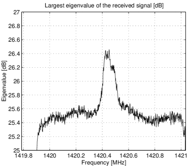
To compare our off-line frequency domain correlation process based on recorded data to the online Westerbork correlator (the DZB) we have made an interference-free observation of the galactic HI absorption of 3C48, a spectral line at 1420 MHz. Figure 14 shows the estimate of the power spectral density of the received signal based on the largest eigenvalue of the covariance matrix.

The coherency (correlation coefficient) of signals $x_{i}$ and $x_{j}$ at the output of telescopes $i$ and $j$ is defined as

$$\rho_{ij}(f)\;=\;\frac{{\rm E}(x_{i}(f)\bar{x}_{j}(f))}{\sqrt{{\rm E}(|x_{i}(f)|^{2}){\rm E}(|x_{j}(f)|^{2})}}\;=\;\frac{R_{ij}(f)}{\sqrt{R_{ii}(f)R_{jj}(f)}}\,.$$ (20)

Since all telescopes are tracking the same source $s$, we have that $x_{i}=\alpha_{i}s+n_{i}$ where $n_{i}$ is the noise at telescope $i$. With uncorrelated noise of power ${\rm E}(|n_{i}|^{2})=\sigma^{2}$, and a source power of $\sigma_{s}^{2}$, it follows that

$$\rho_{ij}(f)=\alpha_{i}\bar{\alpha}_{j}\frac{\sigma_{s}^{2}(f)}{\sigma_{s}^{2}(f)+\sigma^{2}(f)}\qquad(i\neq j)\,.$$

Thus, the theoretical value of the coherency is constant over all nonzero baselines, and can be estimated based on the parameters of 3C48 and knowledge of the receiver gains and noises. These theoretically expected (asymptotic) values can then be compared to the computed coherencies of the recorded observation using (20), and can also be compared to the coherency measured with the DZB hardware.

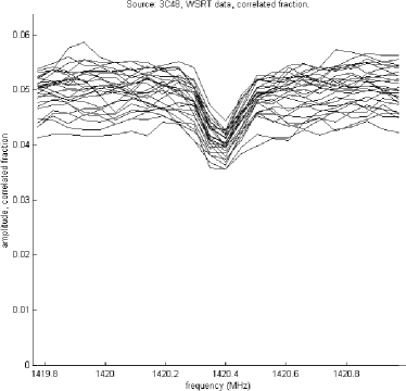
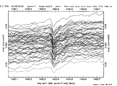
Figure 15$(a)$ shows the magnitude of the coherency function for all nonzero baselines as based on a NOEMI recording of a few seconds. The coherency is around 5%, and the spectral absorption at 1420.4 MHz shows up as a dip. We verified that the absorption line is statistically significant. For comparison we include the same spectral line as processed by the WSRT DZB correlator in figure 15$(b)$. The values of the coherency are in good agreement (differences are due to differences in processing bandwidths, observation times and instrumental settings).

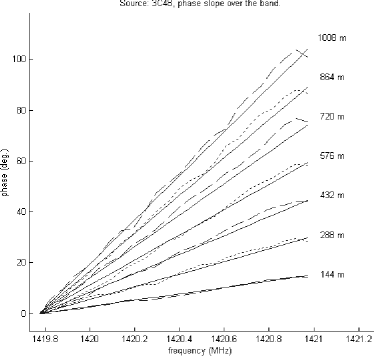
To verify the phase behavior of the coherency we have computed the unwrapped phase as a function of frequency. Note that the geometrical delay compensation and fringe corrections were not included in the recording. Due to the narrowband processing, the delay offset $\tau_{ij}$ of one channel with respect to another shows up as a frequency-dependent phase shift $e^{-j2\pi f\tau_{ij}}$ (the fringe), which will be the phase of $\rho_{ij}(f)$. Here, $\tau_{ij}$ depends on the location of 3C48 and the baseline vector $\mathbf{r}_{i}-\mathbf{r}_{j}$ between antenna $i$ and $j$, and is known. Figure 16 compares the observed phase differences (averaged over all identical baselines) to the computed phase, as a function of frequency and baseline length. It is seen that the correspondence is very good. Note that for the shorter baselines we have more realizations so that their correspondence is better.

7.3 3C48 absorption line with GSM interference

At this point we are ready to demonstrate the performance of the sub-band detection and blanking method as presented in section 5. To this end, we have superimposed on the 3C48 data (at $1420$ MHz) another measurement file containing GSM interference (at $905$ MHz), with the same bandwidth and for various amplitude scalings of each file. Although a bit artificial, the good linearity of the WSRT system implies that had a GSM signal been transmitted with a carrier frequency of $1420$ MHz, then the measured data would be the superposition of the two signals plus system noise. The overlay allows us to verify the blanking performance for various mixtures of signal-to-interference power, since the clean data is now available as a reference and also the theoretical coherency is well known.

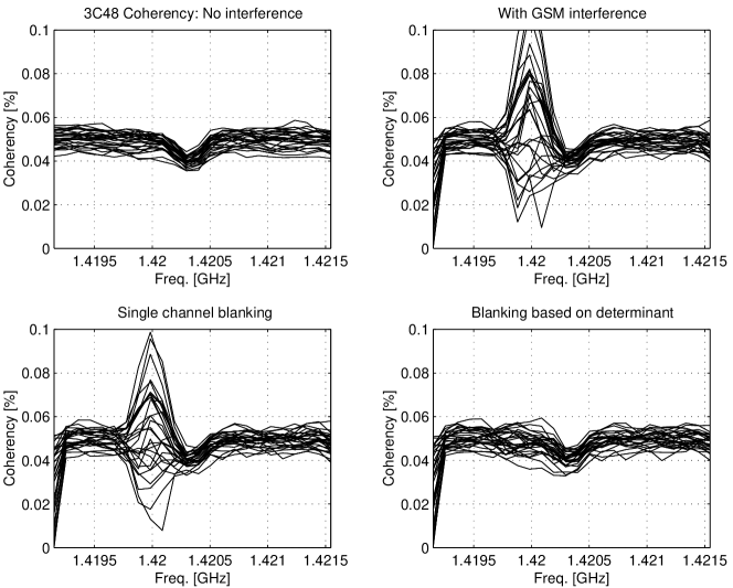
As described in section 5, the detection of an interferer in a specific time-frequency cell is based on the eigenvalues of the corresponding correlation matrix of the resulting mixture. In this scheme, if one or more eigenvalues are above a threshold, then an interferer is detected and that data block is omitted. However, to avoid the selection of the threshold based on a desired false alarm rate, we have chosen to simply throw away the worst 30 percent of the data according to the value of the detector. We have computed the coherency of the clean, the contaminated and the blanked signals. Figure 17 shows the coherency functions over all baselines for a particular mixture of signals and interference: scaling the GSM data file by $0.1$ and the clean 3C48 data file by $0.9$. It is seen that $(a)$ the clean 3C48 spectrum shows the absorption line, which is $(b)$ completely masked when GSM interference is added. After blanking, $(d)$ the absorption line is almost perfectly recovered. For comparison we also included $(c)$ the results of blanking based on single channel power detection from channel 2 only, without the sub-band decomposition. The failure of this common way of single channel detection is clearly seen. The reason is that the GSM signal was rather weak, so that for single-channel wideband processing the probability of detection was quite low, even for a false alarm rate of up to $30\%$.

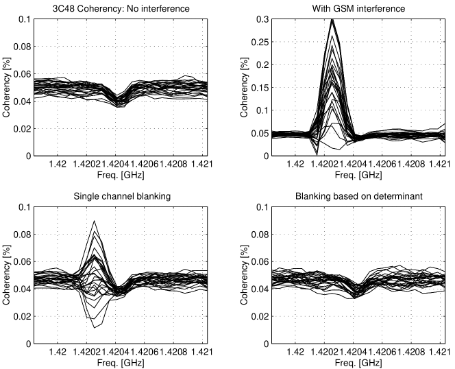
To show the effect of interference power we have repeated the experiment with the GSM data set weighted by a factor $0.5$. The stronger GSM interferer is now more easily detected and the resulting spectrum after blanking is better as seen in figure 18.

8 Conclusions

In this paper, we considered various aspects of multichannel interference suppression for radio-astronomy. It was shown that by sub-band processing we have access to the many narrow-band techniques available in array signal processing. We have demonstrated the benefits of multichannel spatio-spectral blanking, both theoretically and on measured data. The results are very pleasing. We have also discussed spatial filtering techniques and demonstrated how they can be incorporated into the radio-astronomical measurement equation.

$(a)$ \begin{picture}(0.0,0.0) \end{picture}

$(b)$ \begin{picture}(0.0,0.0)\end{picture}

Figure 1: $(a)$ The emitted electrical field from the celestial sphere is received by a rotating telescope array; $(b)$ geometrical delay compensation

\begin{picture}(0.0,0.0)\end{picture}

Figure 2: The astronomical correlation process

Figure 3: Television broadcast

Figure 4: GSM uplink

Figure 5: GSM downlink

Figure 6: Iridium downlink

Figure 7: GPS transmission, showing the civil code (BW$=1.023$ MHZ) superimposed on the wideband military code (BW$=10.23$ MHZ). $f_{c}=1575$ MHz.

Figure 8: $P_{D}$ vs. INR, for $M=10,\;30,\;64$, and false alarm rate $P_{FA}=5\%$

\begin{picture}(0.0,0.0)\end{picture}

\begin{picture}(0.0,0.0)\end{picture}

Figure 9: (a) Interferer with slot length $L=\alpha M$ samples, power $\sigma_{s}^{2}$ per on-sample, and duty cycle $\beta$. (b) Corresponding probability density of interference power in a single analysis window.

Figure 10: (a) Effective residual INR after blanking versus effective INR at the input; (b) fraction of remaining samples after blanking

Figure 11: Eigenstructure as a function of time

\begin{picture}(0.0,0.0)\end{picture}

Figure 12: Estimation of $\mathbf{a}$ using a reference antenna

Figure 13: Overview of main WSRT systems with the NOEMI data recorders

Figure 14: 3C48: largest eigenvalue of the covariance matrix

$(a)$ $(b)$

Figure 15: 3C48 coherency function, magnitude (for all baselines). $(a)$ NOEMI recording and off-line processing, $(b)$ online WSRT processing by the DZB

Figure 16: 3C48 averaged coherency phase function vs. frequency, various baselines.

Figure 17: Magnitude of the coherency functions of 3C48 mixed with GSM interference. GSM data scaled by $0.1$. $(a)$ clean 3C48 data, $(b)$ 3C48 mixed with GSM, $(c)$ after single channel detection/blanking, $(d)$ after multichannel subband detection/blanking

Figure 18: Magnitude of the coherency functions of 3C48 mixed with GSM interference. GSM data scaled by $0.5$. $(a)$ clean 3C48 data, $(b)$ 3C48 mixed with GSM, $(c)$ after single channel detection/blanking, $(d)$ after multichannel subband detection/blanking

References

- Barnbaum Bradley [1998] C. Barnbaum and R.F. Bradley, 1998, AJ, 115:2598.
- Box [1949] G.E.P. Box, 1949, Biometrika, 36:317.
- Friedman [1996] P. Friedman, 1996, In Proc. IEEE signal processing workshop on statistical signal and array processing, (IEEE), 264.
- Haykin [1995] S. Haykin, 1995, Adaptive filter theory. Prentice-Hall.
- Kay [1998] S.M. Kay, 1998, Fundamentals of statistical signal processing: Detection theory. PTR, Prentice Hall.
- Kasper Chute Routledge [1982] B.L. Kasper, F.S. Chute, and D. Routledge, 1982, MNRAS, 199:345.
- Krim Viberg [1996] H. Krim and M. Viberg, 1996, IEEE Signal Processing Magazine, 13(3):67.
- Leshem van der Veen [1998] A. Leshem and A.J. van der Veen, 1998. Technical Report NOEMI-98-01, Delft University of Technology.
- Leshem van der Veen [1999] A. Leshem and A.J. van der Veen, 1999. In Proc. IEEE workshop on higher order statistics, Ceasaria, Israel, (IEEE computers society press), 25.
- Leshem van der Veen [1999b] A. Leshem and A.J. van der Veen, 2000, Radio astronomical imaging in the presence of strong radio interference. To appear IEEE Trans. Information Theory.
- Leshem van der Veen Deprettere [1999c] A. Leshem, A.J. van der Veen, and E. Deprettere, 1999. In Proc. IEEE signal processing advances in wireless communications, (IEEE), 374.
- Maslakovic et al. [1996] S. Maslakovic, I.R. Linscott, M. Oslick, and J.D. Twicken, 1996. In Proc. IEEE int. symposium on time-frequency and time-scale analysis, (IEEE), 349.
- Proakis [1995] J.G. Proakis, 1995, Digital communications. McGraw-Hill, 3rd edition.
- Perley Schwab Bridle [1989] R.A. Perley, F. Schwab, and A.H. Bridle, editors, 1989, Synthesis imaging in radio astronomy. Astronomical society of the pacific.
- Thompson [1982] A.R. Thompson, 1982, The response of radio-astronomy synthesis array to interfering signals. IEEE Trans. AP, 30:450.
- Thompson et al. [1986] A.R. Thompson, J.M. Moran, and G.W. Swenson, 1986, Interferometry and Synthesis in Radioastronomy. John Wiley and Sons.
- Weber et al. [1997] R. Weber, C. Faye, F. Biraud, and J. Dansou, 1997, A&AS., 126(1):161.
- Wax Kailath [1985] M. Wax and T. Kailath, 1985, IEEE Trans. Acoustics, Speech, Signal Processing, 33(2):387.