Photometric Redshifts based on standard SED fitting procedures

Abstract

In this paper we study the accuracy of photometric redshifts computed through a standard SED fitting procedure, where SEDs are obtained from broad-band photometry. We present our public code hyperz, which is presently available on the web. We introduce the method and we discuss the expected influence of the different observational conditions and theoretical assumptions. In particular, the set of templates used in the minimization procedure (age, metallicity, reddening, absorption in the Lyman forest, …) is studied in detail, through both real and simulated data. The expected accuracy of photometric redshifts, as well as the fraction of catastrophic identifications and wrong detections, is given as a function of the redshift range, the set of filters considered, and the photometric accuracy. Special attention is paid to the results expected from real data.

1 Introduction

The estimate of redshifts through photometry is one of the most promising techniques in deep universe studies, and certainly a key point to optimize field surveys with large-field detectors. It is in fact an old idea of Baum (1962), who originally applied it to the measure of redshifts for elliptical galaxies in distant clusters. It was later used by several authors in the eighties (Couch et al. 1983, Koo 1985) on relatively low-redshift samples, observed in the $\sim 4000$ to $8000$ Å domain. Later in the nineties, the interest for this technique has increased with the development of large field and deep field surveys, in particular the Hubble Deep Field North and South (HDF-N and HDF-S).

Basically two different photometric redshift techniques can be found in the literature: the so-called empirical training set method, and the fitting of the observed Spectral Energy Distributions (hereafter SED) by synthetic or empirical template spectra. The first approach, proposed originally by Connolly et al. (1995, 1997), derives an empirical relation between magnitudes and redshifts using a subsample of objects with measured spectroscopic redshifts, i.e. the training set. A slightly modified version of this method was used by Wang et al. (1998) to derive redshifts in the HDF-N by means of a linear function of colours. This method produces small dispersions, even when the number of filters available is small, and it has the advantage that it does not make any assumption concerning the galaxy spectra or evolution, thus bypassing the problem of our poor knowledge of high redshift spectra. However, this approach is not flexible: when different filter sets are considered, the empirical relation between magnitudes and redshifts must be recomputed for each survey on a suitable spectroscopic subsample. Moreover, the training set is constituted by the brightest objects, for which it is possible to measure the redshift. Thus, this kind of procedure could in principle introduce some bias when computing the redshifts for the faintest sources, because there is no guarantee that we are dealing with the same type of objects from the spectrophotometrical point of view. Also, the redshift range between $1.4$ and $2.2$ had been hardly reached by spectroscopy up to now, because of the lack of strong spectral features accessible to optical spectrographs. Thus, no reliable empirical relation can be found in this interval.

The SED fitting procedure, described in detail in the following section, bases its efficiency on the fit of the overall shape of spectra and on the detection of strong spectral properties. The observed photometric SEDs are compared to those obtained from a set of reference spectra, using the same photometric system. The photometric redshift of a given object corresponds to the best fit of its photometric SED by the set of template spectra. This method is used mainly for applications on the HDF, using either observed or synthetic SEDs (e.g. Mobasher et al. 1996, Lanzetta et al. 1996, Gwyn & Hartwick 1996, Sawicki et al. 1997, Giallongo et al. 1998, Fernández-Soto et al. 1999, Arnouts et al. 1999, Furusawa et al. 2000). A crucial test in all cases is the comparison between the photometric and the spectroscopic redshifts obtained on a restricted subsample of relatively bright objects. A combination of this method with the Bayesian marginalization introducing a prior probability was proposed by Benítez (2000).

The aim of this paper is to explain in a straightforward way the expected performances and limitations of photometric redshifts computed from broad-band photometry. This study has been conducted with our public code called hyperz, which adopts a standard SED fitting method, but most results should be completely general in this kind of calculations. This program was originally developed by Miralles (1998) (see also Pelló et al. 1999), and the present version of the code hyperz is available on the web at the following address:

http://webast.ast.obs-mip.fr/hyperz .

The plan of the paper is the following. In Section 2 we present the method used by hyperz and the involved set of parameters. The accuracy of the redshift determinations and the expected percentage of catastrophic identifications, as a function of the filter set and the photometric errors, are studied through simulations in Section 3. The influence of the different parameters on the accuracy of photometric redshifts is investigated in Section 4, using both simulations and spectroscopic data from the HDF. Section 5 is devoted to the analysis on the expected accuracy and possible systematics when exploring real data, coming from deep photometric surveys. A general discussion is given in Section 6 and conclusions are listed in Section 7.

2 The method

Photometric redshifts (hereafter $z_{\rm phot}$) are based on the detection of strong spectral features, such as the $4000$ Å break, Balmer break, Lyman decrement or strong emission lines. In general, broad-band filters will allow to detect only “breaks”, and they are not sensitive to the presence of emission lines, except when their contribution to the total flux in a given filter is higher or of the same order of photometric errors, as it happens in the case of AGNs (Hatziminaoglou et al. 2000).

Filter	$\lambda_{\rm eff}$ [Å]	width [Å]
$U$	3652	543
$B$	4358	987
$V$	5571	1116
$R$	6412	1726
$I$	7906	1322
$Z$	9054	1169
$J$	12370	2034
$H$	16464	2863
$K$	22105	3705
F300W	3010	854
F450W	4575	878
F606W	6039	1882
F814W	8010	1451

Table 1: Characteristics of filters used in the simulations: the effective wavelength $\lambda_{\rm eff}$ and the surface of the normalized response function.

The method used in this paper to compute photometric redshifts is a SED fitting through a standard $\chi^{2}$ minimization procedure, computed with our code hyperz. The observed SED of a given galaxy is compared to a set of template spectra:

$$\chi^{2}(z)=\sum_{i=1}^{N_{\rm filters}}\left[{F_{{\rm obs},i}-b\times F_{{\rm temp},i}(z)\over\sigma_{i}}\right]^{2}\>,$$ (1)

where $F_{{\rm obs},i}$, $F_{{\rm temp},i}$ and $\sigma_{i}$ are the observed and template fluxes and their uncertainty in filter $i$, respectively, and $b$ is a normalization constant.

The new Bruzual & Charlot evolutionary code (GISSEL98, Bruzual & Charlot 1993) has been used to build 8 different synthetic star-formation histories, roughly matching the observed properties of local field galaxies from E to Im type: a delta burst, a constant star-forming system, and six $\mu$-models (exponentially decaying SFR) with characteristic time-decays chosen to match the sequence of colours from E-S0 to Sd. We use the Initial Mass Function (IMF) by Miller & Scalo (1979), but this choice has a negligible impact on the final results, as discussed in Section 4.6. The upper mass limit for star formation is $125\,M_{\odot}$. The basic database includes only solar metallicity SEDs, but other possibilities are discussed in Section 4. The library also includes a set of empirical SEDs compiled by Coleman, Wu and Weedman (1980) (hereafter CWW) to represent the local population of galaxies. CWW spectra were extended to wavelengths $\lambda\leq 1400$ Å and $\lambda\geq 10000$ Å using the equivalent GISSEL spectra. The synthetic database derived from Bruzual & Charlot includes 408 spectra (51 different ages for the stellar population and 8 star-formation regimes). In most applications, there is no sensible gain when the number of $\mu$-models is reduced to only 3, thus including only 255 spectra.

Throughout this paper we use the same set of broad-band filters, with characteristics presented in Table 1. These filters cover all the wavelength domain under study, without major overlap or gap. We also include the HDF filters used in Sections 4 and 5 (from Biretta et al. 1996). The hyperz filter library is an enlarged version of the original Bruzual & Charlot one, and presently includes 163 filters and detector responses. All magnitudes given in this paper refer to the Vega system.

Hyperz has been optimized to gain in efficiency when computing $z_{\rm phot}$ on large catalogues. The input data for a given catalogue are magnitudes and photometric errors. To compute a reliable estimate of $z_{\rm phot}$, the colours and the corresponding photometric errors must be obtained with particular care, including uncertainties due to zero-points, intrinsic accuracy, etc. Magnitudes are obtained within the same aperture in all filters, after correction for seeing differences between images. For a given catalogue, the relevant parameters introduced in the $z_{\rm phot}$ calculation are:

• The set of template spectra. This point includes the SFR type, the possible link between the age and the metallicity of the stellar population, and the choice of an IMF. It is discussed in Section 4.

• The reddening law is usually taken from Calzetti et al. (2000), but 4 other laws are also included in the code. This is discussed in Section 4.4. The input value is $A_{V}$, corresponding to a dust-screen model, with $F_{\rm o}(\lambda)=F_{\rm i}(\lambda)10^{-0.4A_{\lambda}}$, where $F_{\rm o}$ and $F_{\rm i}$ are the observed and the intrinsic fluxes, respectively. The extinction at a wavelength $\lambda$ is related to the colour excess $E_{B-V}$ and to the reddening curve $k(\lambda)$ by $A_{\lambda}=k(\lambda)E_{B-V}=k(\lambda)A_{V}/R$, with $R=3.1$ except for the Small Magellanic Cloud ($R=2.72$) and the Calzetti’s law ($R=4.05$). The normal setting for $A_{V}$ ranges between 0 and $1.5$ magnitudes. The mean galactic extinction correction towards a given line of sight can be introduced in terms of $E_{B-V}$, and it is applied to the whole catalogue.

• Flux decrements in the Lyman forest are computed according to Giallongo & Cristiani (1990) and Madau (1995), both of them giving similar results.

• The limiting magnitude in each filter, and the rule to be applied in the case of non detection. The rule is set for each filter independently, and there are 4 different possibilities: 0) the filter is not taken into account in the computation; 1) the flux in this filter is set to 0 with an error bar corresponding to the flux deduced from the limiting magnitude; 2) the flux in this filter is set to $1/2$ of the limiting flux, according to the limiting magnitude, and the associated 1 sigma error is $\pm 1/2$ times this value; 3) the flux and the 1 sigma error in this filter are computed from the limiting magnitude and from the error associated to the limiting magnitude (both fixed). Case 1 is the usual setting when one is dealing with a relatively deep survey in the considered filter, whereas case 0 applies to “out-of-field” objects. Case 2 and 3 are well suited for relatively shallow surveys. The idea of “shallow” and “deep” in this context refers to relative values of the limiting magnitudes associated to the different filters in the photometric catalogue.

• The cosmological parameters $H_{0}$, $\Omega_{0}$ and $\Omega_{\Lambda}$, which are only related here to the maximum age allowed to the stellar population at a given redshift. The age checking is an option.

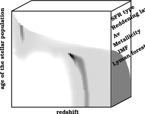
Due to the degeneracy in the parameter space defined by the SFR type, age, metallicity and reddening, the $z_{\rm phot}$ computation for a given object is equivalent to finding the most likely solution for the redshift across this parameter space, regardless to details on the best-fit SED (see Figure 1). Both the $z_{\rm phot}$ and the SED are obtained through hyperz, together with the best fit parameters ($A_{V}$, spectral type, metallicity and age). Because of the degeneracy between these parameters, the relevant information shall be the redshift and the rough SED type, in the sense that a given object has a “blue” or “red” continuum at a given $z$, but no reliable information can be obtained about the other parameters from broad-band photometry alone.

Figure 1: Artist view of the SED fitting procedure to compute $z_{\rm phot}$. The figure presents a likelihood map for a representative object at $z\sim 4$. The shaded area encloses the highest confidence level region according to the $\chi^{2}$ associated probability. Each point on the redshift-age map corresponds to the best fit of the SED obtained across the parameter space. The degeneracy in the parameter space is shown in this example.

3 Filters and photometric accuracy

Figure 2: Comparison between $z_{\rm model}$ and $z_{\rm phot}$ for simulated catalogues with $\Delta m=0.1$ and filters sets BVRI, UBVRI, UBVRIJ, UBVRIK, BVRIJK, UBVRIJHK. Dotted lines correspond to $\Delta_{z}=0.2$, dashed lines to $\Delta_{z}=0.5$ and thin solid lines to $\Delta_{z}=1$.

		$z=0.0$ – 0.4		0.4 – 1.0		1.0 – 2.0		2.0 – 3.0		3.0 – 5.0		5.0 – 7.0
filters	$\Delta m$	$\sigma_{z}$	$\left<\Delta_{z}\right>$	$\sigma_{z}$	$\left<\Delta_{z}\right>$	$\sigma_{z}$	$\left<\Delta_{z}\right>$	$\sigma_{z}$	$\left<\Delta_{z}\right>$	$\sigma_{z}$	$\left<\Delta_{z}\right>$	$\sigma_{z}$	$\left<\Delta_{z}\right>$
	0.05	0.18	0.00	0.22	-0.13	0.32	0.10	0.30	0.07	0.23	0.08	0.16	0.05
BVRI	0.10	0.20	-0.05	0.30	-0.21	0.38	0.08	0.45	0.10	0.25	0.10	0.19	0.07
	0.20	0.29	-0.19	0.37	-0.24	0.41	0.18	0.54	0.01	0.34	0.14	0.23	0.07
	0.30	0.25	-0.34	0.38	-0.24	0.42	0.25	0.53	-0.21	0.35	0.14	0.28	0.09
	0.05	0.07	-0.03	0.17	-0.07	0.26	0.12	0.21	0.04	0.17	0.05	0.18	0.06
UBVRI	0.10	0.09	-0.03	0.21	-0.11	0.35	0.17	0.33	0.11	0.23	0.08	0.19	0.04
	0.20	0.20	-0.11	0.29	-0.19	0.42	0.17	0.41	0.12	0.27	0.09	0.23	0.06
	0.30	0.28	-0.20	0.31	-0.18	0.49	0.16	0.45	0.11	0.29	0.11	0.27	0.07
	0.05	0.04	-0.01	0.11	-0.05	0.25	0.11	0.13	0.04	0.17	0.06	0.09	0.01
UBVRIZ	0.10	0.07	-0.02	0.16	-0.08	0.28	0.11	0.23	0.07	0.22	0.09	0.14	0.02
	0.20	0.17	-0.08	0.22	-0.11	0.41	0.11	0.34	0.16	0.28	0.12	0.19	0.05
	0.30	0.21	-0.12	0.27	-0.15	0.44	0.12	0.40	0.18	0.32	0.15	0.24	0.08
	0.05	0.04	-0.01	0.07	-0.02	0.11	-0.01	0.12	0.07	0.12	0.04	0.11	0.02
UBVRIJ	0.10	0.08	-0.01	0.11	-0.06	0.20	-0.01	0.14	0.10	0.17	0.07	0.15	0.03
	0.20	0.17	-0.09	0.19	-0.08	0.30	0.00	0.23	0.14	0.26	0.13	0.18	0.03
	0.30	0.22	-0.13	0.26	-0.15	0.35	0.01	0.30	0.17	0.30	0.17	0.22	0.06
	0.05	0.04	-0.01	0.07	-0.02	0.11	0.00	0.21	0.07	0.13	0.04	0.15	0.05
UBVRIK	0.10	0.08	-0.02	0.10	-0.05	0.22	0.01	0.27	0.12	0.18	0.08	0.15	0.06
	0.20	0.17	-0.064	0.16	-0.08	0.31	0.01	0.32	0.18	0.22	0.12	0.21	0.08
	0.30	0.22	-0.14	0.25	-0.14	0.36	-0.01	0.35	0.20	0.26	0.14	0.23	0.09
	0.05	0.06	-0.01	0.06	-0.03	0.16	0.00	0.16	0.01	0.13	0.03	0.09	0.03
BVRIJK	0.10	0.12	-0.03	0.11	-0.05	0.24	0.00	0.19	0.02	0.18	0.07	0.12	0.04
	0.20	0.19	-0.06	0.23	-0.07	0.33	-0.04	0.27	0.06	0.23	0.11	0.16	0.07
	0.30	0.25	-0.14	0.26	-0.14	0.40	-0.04	0.32	0.09	0.27	0.16	0.20	0.09
	0.05	0.04	-0.01	0.05	-0.02	0.13	0.02	0.06	0.00	0.12	0.03	0.09	0.02
UBVRIJK	0.10	0.09	-0.01	0.09	-0.03	0.21	0.03	0.11	0.02	0.15	0.05	0.12	0.03
	0.20	0.18	-0.05	0.18	-0.06	0.32	0.03	0.20	0.05	0.18	0.09	0.15	0.05
	0.30	0.23	-0.09	0.24	-0.10	0.33	0.05	0.28	0.08	0.21	0.11	0.19	0.07
	0.05	0.03	0.00	0.05	-0.01	0.10	0.00	0.06	0.00	0.09	0.01	0.09	0.02
UBVRIJHK	0.10	0.10	-0.02	0.10	-0.02	0.20	-0.01	0.13	0.03	0.13	0.04	0.11	0.03
	0.20	0.18	-0.06	0.17	-0.07	0.28	-0.02	0.19	0.06	0.19	0.09	0.16	0.06
	0.30	0.25	-0.12	0.25	-0.11	0.33	-0.04	0.27	0.09	0.23	0.11	0.21	0.09

Table 2: Summary of results obtained on simulated catalogues with a homogeneous redshift distribution as a function of the redshift bin, filters set and photometric errors $\Delta m$. See the text for a complete description.

In this section we study through simulations the quality of the $z_{\rm phot}$ as a function of the filter set, the photometric accuracy and the redshift, i.e. the robustness of the redshift determination and the expected percentage of catastrophic identifications and spurious detections. The aim of this exercise is to study the systematic effects produced by the sampling of the SED and the associated noise coming from photometry. Catastrophic identifications ($l\%$) are those with $|\Delta_{z}|=|z_{\rm model}-z_{\rm phot}|\geq 1$, and such objects are thus lost from their original redshift bin. The accuracy of $z_{\rm phot}$ in a given redshift bin is defined by the mean difference $\left<\Delta_{z}\right>=\sum\Delta_{z}/N$ of the sample with respect to the model redshift, excluding catastrophic identifications, and the standard deviation $\sigma_{z}=\sqrt{\sum(\Delta_{z}-\left<\Delta_{z}\right>)^{2}/(N-1)}$. Spurious identifications ($g\%$) correspond to objects which are incorrectly assigned to a given $z_{\rm phot}$ interval, and thus susceptible to contaminate the statistics within this $z_{\rm phot}$ interval; in this case $|\Delta_{z}|\geq 3\times\sigma_{z}$.

Some of these quantities, in particular $l\%$ and $g$%, depend on assumptions about redshift number counts and photometric depth. For this reason we compute them only for a set of simulations with a more realistic modeling for galaxy counts, according to a Pure Luminosity Evolution (PLE) scenario. We discuss the results as a function of the photometric parameters in Section 5.

Simulated catalogues of $1000$ objects were produced, with a homogeneous redshift distribution, in order to compute the above mentioned parameters as a function of the filter set and photometric accuracy. In all cases, the types and ages assigned to the different galaxies in a redshift bin are randomly chosen from the 8 GISSEL98 template families mentioned above, with solar metallicity. Photometric errors in these homogeneous catalogues are introduced as a noise following a Gaussian distribution of fixed $1\sigma$ in magnitudes for each band (0.05 to 0.3 magnitudes, i.e. $\sim$ 5 to 30 % photometric accuracy), and they are uncorrelated for different filters. For each filter set we study the quality of $z_{\rm phot}$ as a function of the photometric accuracy, In this particular case, photometric errors do not scale with magnitudes. A realistic error distribution is used in Section 5. The value of the visual extinction $A_{V}$ ranges between $0$ and $1$. For each simulated galaxy, hyperz computes a $z_{\rm phot}$ value, as well as the $z_{\rm phot}$ error bars corresponding to $P=68,90,99$% confidence levels, computed by means of the $\Delta\chi^{2}$ increment for a single parameter (Avni 1976). The redshift step used to search solutions between $z=0$ and $z=7$ is $\Delta z=0.05$, with an internal accuracy which is 10 times better. The choice of the primary $z$-step between 0.1 and 0.05 does not affect significantly the results.

Figure 3: Examples of the evolution of the probability distributions associated to $\chi^{2}(z)$ as a function of the filter set and photometric errors, for two simulated objects. Left: $z_{\rm model}=0.282$. Right: $z_{\rm model}=2.396$. Dotted lines refer to $\Delta m=0.3$, dashed lines: $\Delta m=0.2$, solid lines: $\Delta m=0.1$. The vertical line marks the true $z_{\rm model}$ value.

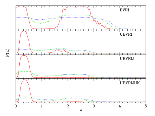
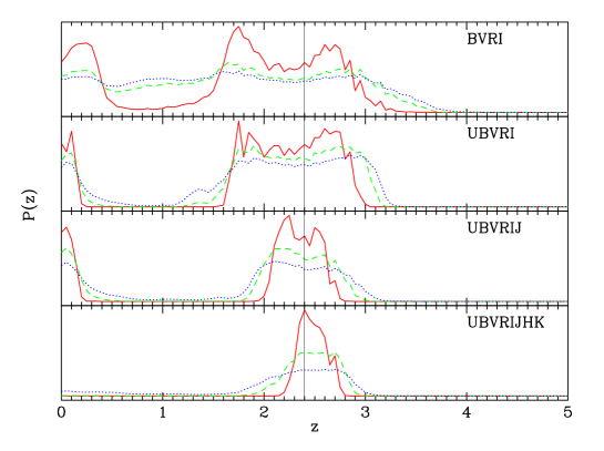
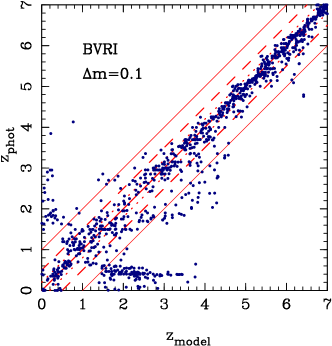
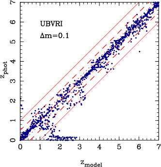
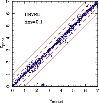
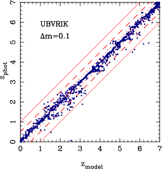
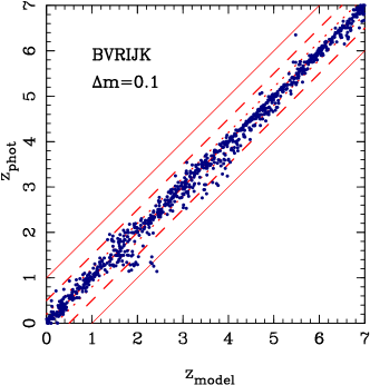
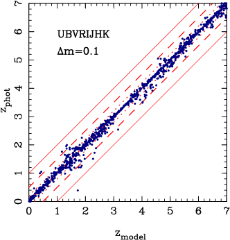
Figure 2 shows the behaviour of the different sets of simulated samples when the $z_{\rm phot}$ is compared to the true $z_{\rm model}$. The results of these simulations are summarized in Table 2. Without near-IR photometry, the errors on individual galaxies become huge at $1.2\leq z\leq 2.2$ as expected due to the lack of strong spectral features in the visible band. In particular, in this redshift range the 4000 Å break goes out of the $I$ band and the Lyman break does not yet affect the photometry in the filter $U$. This problem is solved when near-IR is included. In fact, $J$, $H$, and $K$ filters allow to bracket the 4000 Å break. Also, the lack of $U$ band photometry introduces an enhanced uncertainty in the $z\leq 0.4$ domain (mainly because of the contribution at $z\la 0.2$), because at $z\leq 0.2$ none of the other filters is able to detect a strong break.

All these results are almost independent on the type of galaxy, provided that the evolving population of stars is older than a few $\sim 10^{7}$ years typically. This point is discussed in details in next section.

The dispersion in $z_{\rm phot}$ is strongly sensitive to the photometric uncertainties. There is no significant gain for $\Delta m\leq 0.05$ magnitudes (about $5$% accuracy). This value roughly corresponds to the typical photometric uncertainties in deep photometric surveys, when all the error sources are included. The dispersion and the number of multiple solutions with similar weight rapidly increase up to $\Delta m\sim 0.3$ magnitudes. Including near-IR JHK photometry strongly reduces the error bars within the $1.2\leq z\leq 2.2$ range, without significantly improving the uncertainties in $z_{\rm phot}$ outside this interval. If the filter $Z$ is considered in addition to the five optical filters, the resulting dispersion at low redshift become smaller up to $z_{\rm model}\simeq 1.5$, but the degeneracy at $z_{\rm model}=1.5$ – $3$ still remains, even if less dramatic.

In Figure 3 we illustrate the probability functions for two simulated galaxies at low and high redshift: the solution becomes better constrained around the model value and the degeneracy between high and low redshift solutions disappears with increasing photometric accuracy and when the wavelength range extends up to the near infrared region.

The typical dispersion in $z_{\rm phot}$ obtained here is similar to the values found in the literature, even when the techniques used are appreciably different (Brunner et al. 1997, Connolly et al 1997, …). In most published studies it is extremely difficult to compare the accuracy of $z_{\rm phot}$ as a function of photometric errors.

These results are useful to understand the general trends expected from a given configuration of filters and photometric accuracy. Nevertheless, $z_{\rm phot}$ techniques are often applied to statistical studies, which require more “realistic” simulations in order to define the right observational strategy for the photometric survey. Then, a realistic redshift distribution is needed. For most applications, a PLE model is enough to determine the main trends. Also, photometric uncertainties have to be scaled with magnitude, to reproduce the behaviour of real catalogues. These points are discussed in Section 5.

4 Influence of the different parameters on $z_{\rm phot}$ accuracy

4.1 Templates and Lyman forest blanketing

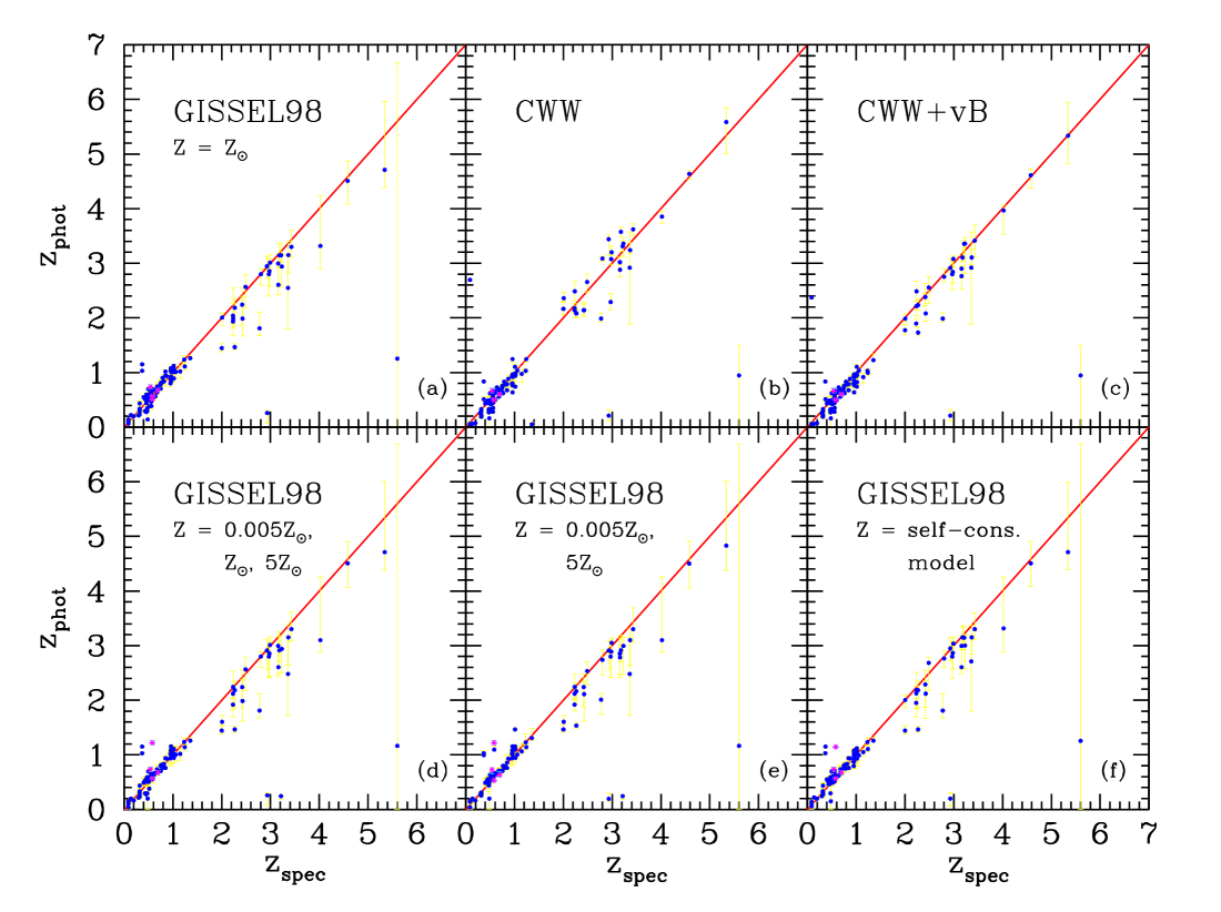
We have studied the influence of the set of templates used on the final results through a comparison between the hyperz $z_{\rm phot}$ determinations and real spectroscopic data on HDF. All the other parameters are fixed in this case, and the only difference is the set of templates used to compute $z_{\rm phot}$. Table 3 summarizes these results. A similar blind test was recently performed by Hogg et al. (1998) on a sample of HDF-N galaxies at $z<1.4$, using different procedures and, in particular, different sets of templates.

We have computed photometric redshifts for the sample of 108 galaxies on the HDF-N with observed $z_{\rm spec}$ (Cohen et al. 1996; Cowie 1997; Zepf et al. 1996; Steidel et al. 1996; Lowenthal et al. 1997) considered by Fernández-Soto et al. (1999) plus 4 galaxies from HDF-S (Glazebrook et al. 2000, in preparation). Among these, 83 galaxies are at $z<1.5$ and 29 at $2<z<6$. Photometry was obtained from the Stony Brook’s group (Fernández-Soto et al. 1999, SUNY web pages http://www.ess.sunysb.edu/astro/hdfs) using the package SExtractor (Bertin & Arnouts 1996) to detect sources, and consists in 7 filters for the HDF-N (F300W, F450W, F606W, F814W plus near infrared photometry in JHK filters obtained by Dickinson et al. 1998 at the KPNO IRIM camera) and 12 for the HDF-S (F300W, F450W, F606W, F814W, plus an additional shallow optical catalogue UBVRI from NTT SUSI2, and near infrared JHK data obtained with NTT SOFI). Here we consider results obtained using the 7 filters for the HDF-N galaxies and all the 12 available filters for the four objects of the HDF-S subsample. Calculations on the HDF-S using 7 filters do not affect significantly the individual photometric redshift and the overall statistic.

To calculate magnitudes from the available measured fluxes in the catalogues, we considered as non-detection criterion a signal-to-noise ratio $S/N<1$. In this case we assigned a magnitude $=99$ and we used the information about the limiting magnitude in the involved filter.

Three different sets of templates are considered in this section: the basic 5 GISSEL98 models with solar metallicity mentioned above (1 delta burst, 3 $\mu$-decaying, 1 constant star-formation system), the CWW set of empirical SEDs, and the CWW set extended with a SED of a very blue galaxy taken from GISSEL library (Miller & Scalo IMF, constant SFR, ${\rm age}=0.1$ Gyr). Adding new very blue spectra to the third set does not change perceptibly the results. As for the simulated catalogues, we search solutions in the redshift interval $z=0$ – $7$ with a step $\Delta z=0.05$. In all cases, a crude limit in absolute magnitude has been imposed to compute $z_{\rm phot}$, with $M_{B}\in[-28,-9]$. Moreover, we checked the age of the template to be consistent with the age of the universe at the considered redshift, depending on the cosmological model. Here we use $\Omega_{0}=1$, $\Omega_{\Lambda}=0$ and $H_{0}=50\,{\rm km\,s^{-1}\,Mpc^{-1}}$. The reddening is assumed to range from $A_{V}=0$ to $1.2$, following the Calzetti et al. (2000) law.

The comparison between $z_{\rm spec}$ and $z_{\rm phot}$ for the 112 galaxies of the sample is shown in Figure 4, for the three sets of templates hereafter referenced as (a), (b) and (c), respectively. Each of them produces a fairly good agreement with the measured spectroscopic redshifts, but noticeable differences appear when considering the values of the dispersion, computed as

$$\delta_{z}=\frac{\sigma}{1+\left<z\right>}=\sqrt{\frac{\sum_{i=1}^{N}|z_{{\rm phot},i}-z_{{\rm spec},i}|^{2}}{N-1}}\frac{1}{1+\left<z\right>}\>,$$

in the two redshift domains ($z<1.5$ and $2<z<6$):

• for $z_{\rm spec}<1.5$ ($\left<z\right>\simeq 0.65$) we found: (a) $\delta_{z}=0.09$; (b) 0.21; (c) 0.17. If we exclude objects with $|z_{\rm phot}-z_{\rm spec}|>0.5$, the value of $\delta_{z}$ reduces to $0.06$ in case (a) (81 objects), and to $0.08$ for (b) and (c) (81 and 82 objects respectively). In case (a), these rejected objects correspond to the two galaxies with uncertain spectroscopic redshifts (see Arnouts et al. 1999). Thus, using GISSEL models in this redshift domain produces more accurate results than CWW templates alone.

• in the high redshift domain, the dispersion in all the considered cases is $\delta_{z}=0.26$ ($\left<z\right>\simeq 3.06$). If we remove catastrophic identifications (2 objects), characterized by $|z_{\rm phot}-z_{\rm spec}|>1$, then $\delta_{z}=0.10$ in case (a), $0.08$ in (b) and $0.07$ in (c). In this case, the CWW set produces slightly better results than GISSEL, probably due to a Lyman blanketing effect. This point is discussed below.

Figure 4: Comparison between photometric and spectroscopic redshifts for the HDF spectroscopic sample. Error bars in $z_{\rm phot}$ correspond to $3\sigma$. Different sets of template spectra are used in the various panels: (a) the basic 5 GISSEL98 models with solar metallicity; (b) the CWW set of empirical SEDs; (c)the CWW set extended with a SED of a very blue galaxy. The lower panels (d), (e) and (f) present the comparison between template sets of different metallicities. See text for more details.

		$z_{\rm spec}<1.5$		$2<z_{\rm spec}<6$
		$\delta_{z}$	$\delta_{z}$	$\delta_{z}$	$\delta_{z}$
Template set		(all, $N=83$)	(non-cata.)	(all, $N=29$)	(non-cata.)
GISSEL ($Z_{\odot}$)	(a)	0.09	0.06(81)	0.26	0.10(27)
GISSEL ($Z_{\odot}$, no $A_{V}$ )		0.13	0.07(81)	0.50	0.13(19)
GISSEL ($Z_{\odot}$, low Lyman blanketing)		0.09	0.06(81)	0.25	0.09(27)
CWW	(b)	0.21	0.08(81)	0.26	0.08(27)
CWW $+$ vB	(c)	0.17	0.08(82)	0.26	0.07(27)
GISSEL ($0.005Z_{\odot}$,$Z_{\odot}$,$5Z_{\odot}$)	(d)	0.10	0.05(80)	0.30	0.11(26)
GISSEL ($0.005Z_{\odot}$,$5Z_{\odot}$)	(e)	0.10	0.06(79)	0.30	0.10(26)
GISSEL self-consistent models	(f)	0.09	0.05(80)	0.26	0.10(27)

Table 3: Summary of dispersions in the HDF $z_{\rm phot}$ measurements for the different sets of templates, where $\delta_{z}=\sigma/\left[1+\left<z\right>\right]$, using the Calzetti’s law with $A_{V}$ ranging from 0 to 1.2 magnitudes. The total number of objects considered in each non-catastrophic sample is given in brackets. See more details in text.

In general, the reasons of failures can be ascribed to many effects, such as a wrong photometry (systematic errors when measuring magnitudes or underestimated photometric errors) leading to a highly unlikely fit, or a probability function with significant secondary peaks, because of degeneracy among the fit parameters, or a relatively “flat” probability function due to a lack of sufficient photometric information. The last explanation applies particularly to the object at $z_{\rm spec}=5.64$, which is detected only in filter F814W and which is at the limit of detection in F450W, with $S/N\simeq 1.5$. However, if we use all the available photometry, disregarding the $S/N$ criterion, we obtain $z_{\rm phot}=5.13$. The object at $z_{\rm spec}=2.931$ is placed at low redshift by other groups (Fernández-Soto et al. 1999, Arnouts et al. 1999). Nevertheless a secondary peak, with a very small $\chi^{2}$ probability, is found at $z=2.90$.

We can remark that at high redshift the cases (b) and (c) are better centred around the spectroscopic value. However, their $\chi^{2}$ values are higher than in case (a). The reason suspected for that is the one-to-one relation introduced here between the Lyman-forest absorption and the redshift. We investigate this problem by assigning different values to the Lyman-forest decrement, multiplying the values of the mean line blanketing $\left<D_{A}\right>$ and $\left<D_{B}\right>$ provided by Madau (1995) by a factor 0.5 and 1.5, then increasing or decreasing the absorption (Furusawa et al. 2000). We found a better fit to the HDF data when the Lyman forest along the line of sight produces a smaller flux decrement with respect to the mean value. In this case we obtain $\delta_{z}=0.09$ for the GISSEL case (a), a value which is similar to the value of CWW SEDs. An overestimate of absorption due to neutral hydrogen induces a subsequent and systematic underestimate of redshifts, because the same attenuation of the flux could be reproduced with a solution at lower redshift. Hence a careful knowledge of the UV region of SEDs is essential to accurately assess $z_{\rm phot}$; furthermore, the Lyman forest represents the most important signature of spectra in the high redshift regime. Thus it is important to allow the blanketing in the Lyman forest to span a sufficiently wide range of values in order to prevent systematic effects at high-$z$, which could depend on the line of sight.

It is worth to notice that, even if all the template SEDs reproduce the spectroscopic redshifts on the HDF with sufficient accuracy, the redshift distributions of galaxies could change significantly when we are dealing with objects fainter than the spectroscopic limits, for which no training set is available. When the redshift distribution obtained on the HDF with CWW templates is compared with the equivalent one computed with GISSEL templates, there are no strong differences in the overall distribution. Nevertheless, this result could not apply to all cases. A straightforward example is the case of a deep photometric survey using visible filters only, without near-IR photometry, and designed to probe the low surface-brightness regime. It is easily shown that, in this case, a degenerate solution could exist for the faintest “blue” sources, for which it is impossible to decide between a low-$z$ solution (low surface-brightness object with a very young stellar population, as presented in next subsection) and a relatively bright $1<z<2.5$ galaxy, with ongoing star-formation (no strong signatures on a continuum increasing bluewards). In that case, using the CWW templates alone will tend to select the later solution systematically, whereas including templates spanning a wide range of ages for the stellar population (such as GISSEL) could select the former solution, thus leading to a completely different redshift distribution. We prefer to adopt a relatively large number of GISSEL’s templates, to supply a wide baseline for modeling the age effects, rather than to assume the evolution reproduced by the transformation in a different local spectral type.

4.2 Age of the stellar population

Photometric redshifts are efficient when a spectral feature is detected through the filters with an important strength as compared to photometric uncertainties. When we are dealing with the stellar continuum of a young stellar population, the $4000$ Å break becomes visible at $\sim 10^{7}$ years (see Bruzual & Charlot 1993). In most cases, this lack of strong features could not be compensated by the presence of strong emission lines, simply because such lines have a negligible effect on the integrated energy when using broad-band filters (see Section 4.7).

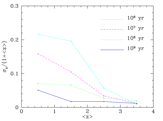
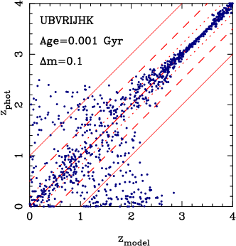
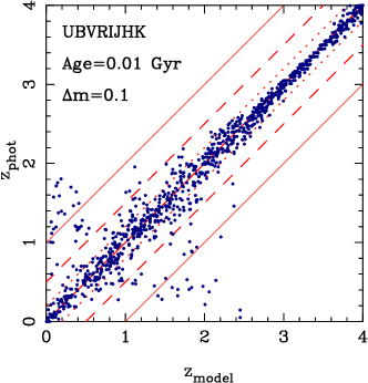
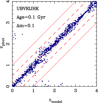
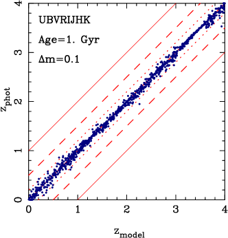
In order to study the effects of age on $z_{\rm phot}$ estimates as a function of redshift, we have produced different sets of catalogues corresponding to different ages, all of them with a uniform distribution in $z$ for the delta burst SED (single stellar population model). Figure 6 displays the general trends of $z_{\rm phot}$ versus $z_{\rm model}$ for representative ages and the UBVRIJHK set of filters. In this case the set of templates used is the basic GISSEL one with solar metallicity. At $z_{\rm model}\ga 3$, the redshift determination is accurate for any age because of the presence of Lyman break in the filter $U$. At smaller redshifts, $z_{\rm phot}$ is based on the 4000 Å break as the strongest spectral signature, and it is visible only in systems which are a few $\sim 10^{7}$ years old.

The results obtained applying hyperz to these catalogues are summarized in Figure 5, where we show the effect described above by means of the dispersion in four redshift bins: the value of $\sigma_{z}/(1+\left<z\right>)$ decreases increasing the redshift and the age of the stellar population.

Figure 5: The dispersion $\sigma_{z}/(1+\left<z\right>)$ as a function of the mean redshift of the considered range. Ages are $10^{6},10^{7},10^{8},10^{9}$ and $10^{10}$ yr from top to bottom.

Figure 6: Comparison between $z_{\rm model}$ and $z_{\rm phot}$ for simulated catalogues of single burst galaxies with $\Delta m=0.1$, filters set UBVRIJHK and ages of galaxies $10^{6},10^{7},10^{8}$ and $10^{9}$ yr.

4.3 Cosmology

The effects of cosmological parameters ($H_{0}$, $\Omega_{0}$ and $\Omega_{\Lambda}$) are only related to the age allowed to the stellar population at a given redshift. When using hyperz, the age of the stellar population can be optionally limited to the age range permitted by the cosmological parameters. In order to quantify such effect on $z_{\rm phot}$, if any, we have compared the results previously obtained on the HDF (with the crude age limitation given above) with those obtained without age constraints, and also with a different set of cosmological parameters ($\Omega_{0}=0.3$, $\Omega_{\Lambda}=0.7$ and $H_{0}=50\,{\rm km\,s^{-1}\,Mpc^{-1}}$). These results show that the effect of the cosmological parameters on the $z_{\rm phot}$ estimate is negligible, because they affect $\delta_{z}$ by less than $1$%.

4.4 Reddening

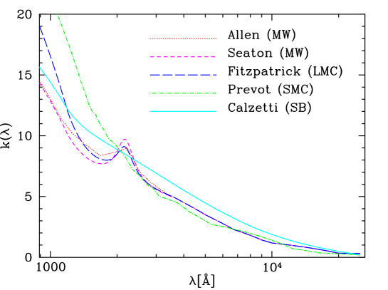
The five reddening laws presently implemented in hyperz are:

1. Allen (1976) for the Milky Way (MW);

2. Seaton (1979) fit by Fitzpatrick (1986) for the MW;

3. Fitzpatrick (1986) for Large Magellanic Cloud (LMC);

4. Prévot et al. (1984) and Bouchet et al. (1985) for Small Magellanic Cloud (SMC);

5. Calzetti et al. (2000) for starburst galaxies.

The different laws are presented in Figure 7.

Figure 7: Extinction curves $k(\lambda)$ for the different reddening laws implemented in hyperz.

Recent studies on high redshift galaxies and star formation obscured by dust have shown the importance of reddening in the high-$z$ universe. In order to probe this issue on $z_{\rm phot}$ computations, we have compared the results previously obtained on the HDF to those obtained assuming no reddening, all the other parameters being fixed. We found $\delta_{z}=0.13(0.07$ without catastrophic objects) for the low-$z$ bin and $\delta_{z}=0.50(0.13)$ for the high-$z$ one, but with a much higher percentage of catastrophic identifications: 10 objects at $z_{\rm spec}\simeq 3$ are erroneously identified as low redshift galaxies.

Therefore, keeping a wide range of reddening values seems to be essential to reproduce the SEDs of high redshift galaxies. According to Steidel et al. (1999), the typical $E_{B-V}$ for galaxies to $z\sim 4$ is $0.15$ mags, thus $A_{V}\simeq 0.6$ mags when using a Calzetti’s law. The maximum $A_{V}$ allowed in our calculations is about 2 times this value.

Moreover, we conducted a test to study the influence of the different reddening laws, using all the implemented possibilities. We found that the laws reproducing the extinction of the Milky Way and the Large Magellanic Cloud are not appropriate to fit the SEDs of high redshift galaxies ($z_{\rm spec}>2$), whereas they leave the low redshift region unaffected. Instead, the fourth law, corresponding to the Small Magellanic Cloud, produces results similar to those obtained with the curve provided by Calzetti et al. (2000). It correctly assigns the $z_{\rm phot}$ to the high redshift objects, but it places a couple of low $z_{\rm spec}$ objects at higher $z_{\rm phot}$. The last effect is probably due to the higher and steeper $k(\lambda)$ at short wavelength as compared to Calzetti’s, which mimics the additional effect of the UV attenuation induced by the Lyman forest. At high redshift, the most important wavelength region is the UV, between $1000$ Å and $3000$ Å, where the considered laws give quite different trends, thus modifying in a different way the magnitudes and producing different values of $\chi^{2}$. In fact, most of the fits to the HDF sample using reddening laws from 1 to 4 produce worse $\chi^{2}$ values than the Calzetti’s law, in particular for those objects requiring $A_{V}>0.6$. These galaxies cannot be reproduced by the MW and LMC laws, even when the limit of $A_{V}$ is increased up to $A_{V}=2$.

Thus, the slope of the selected reddening law at short wavelengths must be defined carefully; the extrapolation used here to extend the laws 1 to 4 towards wavelengths not covered by data is rather poor. These considerations get stronger evidence that the modeling of the UV region of SEDs is essential to recover correctly the high $z$ galaxies. The re-emission of energy coming from dust heated by massive star formation does not affect the present results, because we concentrate on the UV to near-IR bands.

4.5 Metallicity

We have also checked the influence of the metallicity on the $z_{\rm phot}$ estimates using the same HDF training sample. The same computations have been done using different and extreme assumptions for the metallicity of the stellar population, with values ranging from $0.005Z_{\odot}$ to $5Z_{\odot}$ (as allowed by Bruzual & Charlot’s models). We have also developed a self-consistent set of templates, where the evolution in metallicity of the stellar population is explicitly taken into account (cf. Mobasher & Mazzei 1999). In other words, there is a natural link between the age of the stellar population and its mean metallicity. For all metallicity cases, we have built up the same closed-box systems presented before: a constant star-forming galaxy and six $\mu$-models.

Three sets of templates were considered: the 3 different metallicities together (solar and the 2 extreme values), the two extreme values alone, and the self-consistent model. A comparison among all these cases is given in Figure 4 (d,e,f). The dispersions at low redshift without failed objects are $\delta_{z}=0.05,0.06,0.05$ respectively, for the 3 different sets. At high redshift we found $\delta_{z}=0.11,0.10,0.10$, under the same assumptions. A slight improvement on the accuracy of $z_{\rm phot}$ at $z\la 1.5$ is observed when several different metallicities are used together, and the self-consistent model (f) produces the best fit in this redshift range. On the other side, including different metallicities does not affect the high redshift determinations.

4.6 Initial Mass Function

The influence of the IMF has also been tested on the HDF spectroscopic sample. We have used the self-consistent modeling, which takes into account the evolution in metallicity of the stellar population and produces the best fit to the HDF data when using the Miller & Scalo IMF (1979). We have built up the same closed-box models for 2 additional IMFs, Salpeter (1955) and Scalo (1986), keeping the same upper mass limit for star formation. When applying these new templates to the HDF sample, we find exactly the same results in terms of $z_{\rm phot}$ accuracy. Looking more carefully to the results obtained for individual objects, we find that the $z_{\rm phot}$ estimates are approximatively the same, whatever the IMF used. This result is easy to understand because the changes induced on the stellar continuum by the different IMF slopes are compensated in most cases by the other parameters (reddening, age, …), thus giving the same $z_{\rm phot}$ result but a different solution in the parameter space.

When we compute $z_{\rm phot}$ on simulated data, the $z_{\rm phot}$ accuracy is the same when we use a unique IMF in model galaxies and templates and when we use a different IMF in both settings. In addition, we have checked on possible systematic changes on the spectral types derived by hyperz in the later case, with negative results. In particular, a model catalogue built with Miller & Scalo IMF was analysed with Salpeter and Scalo IMFs, and the results were the same as in the Section 4.8 below. This strengthens the idea of the IMF being a secondary parameter in $z_{\rm phot}$ estimates.

4.7 Emission lines

As long as we are dealing here with broad-band photometry, the presence of emission lines on the spectra has a relatively small effect on the integrated fluxes, and thus a small influence on the $z_{\rm phot}$ results. This can be easily quantified when we consider the sample of blue compact galaxies at $z\leq 1.4$ studied by Guzmán et al. (1997), and the samples of star-forming galaxies described by Cowie et al. (1995), Glazebrook et al. (1995) and Terlevich et al. (1991). At relatively low redshift, the main emission lines to consider are [Oii]$\lambda 3727$, H${\alpha}$, H${\beta}$ and [Oiii]$\lambda\lambda 4959,5007$, [Oii] and H${\alpha}$ being the most important contributions to the integrated fluxes. According to Guzmán et al. (1997), the [Oii]$\lambda 3727$ luminosity of star-forming galaxies can be approximated by $L(\mbox{[O{\sc ii}]})\sim 10^{29}W_{\mbox{[O{\sc ii}]}}L_{B}$, where $W_{\mbox{[O{\sc ii}]}}$ is the equivalent width and $L_{B}$ is the blue luminosity in solar units.

For our purposes, an emission line can be overlooked when $f(\mbox{e-line})/f_{\lambda}\leq 1-10^{-0.4\Delta m}$, where $f(\mbox{e-line})$ and $f_{\lambda}$ are, respectively, the integrated fluxes within the emission line and the stellar continuum through the filter, and $\Delta m$ is the photometric uncertainty in magnitudes. A realistic value of $\Delta m\sim 0.05$ to 0.1 mags ($\sim 5$ to 10% uncertainty) imposes $f(\mbox{e-line})/f_{\lambda}\leq 0.05$ to 0.1. The limit in equivalent width for galaxies in the Guzmán et al. sample is a few times $100$ Å, thus most compact star-forming galaxies fulfill this condition. Even when we consider the typical luminosities of vigorous star-forming sources ($L({\rm[O\mbox{\sc ii}]})\sim 10^{42}$ erg/s, Cowie et al. 95, Glazebrook et al. 1995), emission lines are found to be negligible in most of them. Also the large majority of Hii galaxies in the Terlevich et al. (1991) local sample fulfill the condition.

Thus, emission lines do not seem to influence significantly the $z_{\rm phot}$ results on star-forming galaxies. On the contrary, this is not the general case when we are dealing with AGNs, or when the photometry is obtained through narrow-band filters. We have not considered here neither the contribution of AGN to the simulated samples, nor the influence of such templates on the final accuracy when we are dealing with real data. AGN SEDs could be easily introduced in our present scheme, and this particular application is presently under development (Hatziminaoglou et al. 2000).

4.8 Recovering the main SED parameters through hyperz

As mentioned before, hyperz allows to obtain the $z_{\rm phot}$ and the best fit parameters across the whole space. The fitting procedure does not favour any parameter in particular. The homogeneous simulations presented in Section 3 could be used to briefly discuss on the efficiency to recover the most relevant input parameters: the spectral types, the age of the stellar population and $A_{V}$. Because of the degeneracy between these parameters, and the lack of spectral resolution, we only expect a rough spectral type to be retrieved from broad-band photometry. We have considered the 8 spectral types presented in Section 2 to illustrate the case. A general trend appears when comparing the model and retrieved spectral types, whatever the redshift, filter combination and photometric accuracy, with single bursts and early types being more easily identified than late types at all redshifts. Figure 8 displays an example obtained with the UBVRIJK filter combination and 10% photometric accuracy, excluding catastrophic identifications (less than 1% in this case). The trend remains the same whatever the distribution in types, from these detailed 8 types to a rough Burst-E/S/Im distribution. Lowering the $S/N$ or the number of filters slightly increases the trend in terms of contrast between the early type and late type behaviour. Late type misidentifications are due to the degeneracy between age of the stellar population and spectral type, such galaxies being incorrectly assigned to younger and earlier types. In other words, there is often a burst-like template, of suitable age and length, which is able to fit the dominant stellar population of a galaxy observed through broad-band filters. The results are the same whatever the configuration in the parameter space, in particular, changing the order or the position of the different templates in the space produces the same results. Degenerate solutions in the redshift dimension are systematically displayed by hyperz, but this is only an option for the other dimensions of the parameter space. There is no systematic trend in the case of catastrophic identifications, but more than 90% of such objects in these simulations have misidentified spectral types as well.

In the case of $A_{V}$, the procedure will choose the best and the lowest possible value. The results in this case are much better, whatever the $S/N$, provided that near IR filters are included. Using a grid of $\Delta A_{V}=0.2$ to explore the parameter space, the typical value of $\sigma_{AV}=\sqrt{\sum(\Delta_{AV}-\left<\Delta_{AV}\right>)^{2}/(N-1)}$ ranges between $\sigma_{AV}=0.15$ and $0.3$, for photometric accuracies between 5 and 30%, for all the filter combinations including $J$, $H$ or $K$ (or a combination of them). In all the other cases, $\sigma_{AV}=0.3$ to 0.45, for photometric accuracies between 5 and 30%. These values are an average through all the spectral types and redshifts, excluding catastrophic identifications. Similar estimates on catastrophic objects show an increase between $+0.05$ and $+0.3$ on $\sigma_{AV}$, depending on the filter set.

Figure 8: Comparison between the model spectral types and the best-fit templates recovered by hyperz, for the simulations computed in Section 3. Spectral types, from 1 to 8, correspond to galaxies ranging from early (Bursts/E) to late (Im) types. Circle sizes scale with the number of objects. Ideally only the diagonal region should have been populated.

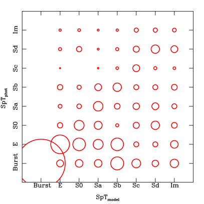
In summary, it is difficult to obtain detailed information on the spectral types from broad-band photometry alone, and this is probably the result of the poor spectral resolution. Near IR photometry allows to constraint the $A_{V}$ value for all spectral types. Only early type galaxies could be reliably identified by this method. For later types, only a rough estimate of the SED type could be obtained, in terms of “blue” or “red” continuum. The classification in this case shall either include the spectral type and the age of the stellar population, or be based on a simple set of templates such as CWW.

5 Expected accuracy on real data

In order to discuss on the expected accuracy and possible systematic errors when exploring real data, we have performed a complete set of simulated catalogues, with a more realistic (non uniform) redshift distribution and $S/N$ ratio along the SEDs. We have adopted the simple PLE model proposed by Pozzetti et al. (1996, 1998), with minimal changes, to derive the redshift distributions and to assign a magnitude to each object in the different filters. Four galaxy types (exponentially decaying SFR with characteristic time $\tau=1$ Gyr and $10$ Gyr, constant SFR with evolution in time and at a fixed age of $0.1$ Gyr) and their corresponding luminosity functions are used to reproduce the number of galaxies expected at a given redshift and absolute magnitude $M_{b_{\rm J}}$. Apparent magnitudes are computed from the evolved SEDs, with ages depending on the redshift considered, the formation redshift, set to $z_{\rm form}=7$, and the cosmological parameters. Photometric errors are scaled to apparent magnitudes assuming the approximate relation $\Delta m\simeq 2.5\log[1+1/(S/N)]$, where $S/N$ is the signal to noise ratio, which is given as a function of the apparent magnitude through $S/N=(S/N)_{0}10^{-0.4(m-m_{0})}$, $(S/N)_{0}$ being the signal to noise ratio at a given reference magnitude $m_{0}$. For simplicity, the photometric error is assigned to the apparent magnitude $m$ according to a Gaussian distribution of $\Delta m$ fixed $\sigma$. This relation is set to reproduce the rapid increase of uncertainties when approaching the limiting magnitudes. According to these equations, a value of $S/N=10$, corresponding to $\Delta m\simeq 0.1$, is reached $2.5$ magnitudes brighter than the magnitude corresponding to $S/N=1$. An object with $S/N<1$ is non-detected in the involved filter ($m=99$). An object is included in the final catalogue if it is detected in the filter $I$ (assuming that this is the selection filter), and in at least two other filters. The last requirement is needed to compute $z_{\rm phot}$.

Filter	$m_{\rm lim}$(d)	$m_{\rm lim}$(s)	Filter	$m_{\rm lim}$
$U$	29.0	25.5	F300W	29.0
$B$	30.0	26.5	F450W	30.5
$V$	29.5	26.0	F606W	30.0
$R$	29.5	26.0	F814W	29.0
$I$	28.5	25.0	$J$	25.0
$Z$	27.5	24.0	$H$	24.0
$J$	25.0	21.5	$K^{\prime}$	23.5
$H$	24.0	20.5
$K$	23.5	20.0

Table 4: Limiting magnitudes at $S/N=1$: (d) deep pencil beam-like survey, (s) shallow ground-based survey.

The same filter combinations discussed in Section 3 have been used to produce the new simulated catalogues. The simulations in Section 3 represent an ideal case, with an infinite depth and a fixed photometric error, disregarding the dependence on errors versus magnitudes. However, the relevant quantities $\sigma_{z}$, $l$% and $g$% strongly depend on the number of objects in each redshift bin and then on the limiting magnitudes.

To give a qualitative idea of the accuracy expected with different observational configurations, we consider two representative cases.

5.1 Deep pencil beam surveys

Firstly, we focus on simulations obtained in the case of a pencil beam-like survey, i.e. a very deep observation, covering a small area. From the photometric point of view, the main improvement with respect to the uniform distributions presented above is that we can introduce, for each object, a realistic $S/N$ in the different filters, with different values from filter to filter. We assume that the detection limit is reached ($S/N=1$) at magnitudes similar to the limiting magnitudes of the HDF, as reported in the column $m_{\rm lim}$(d) of Table 4 and in the right part of the same table for the HDF-N filters. To obtain approximately the same number of galaxies observed in the HDF, a field of 5 arcmin² has been simulated. The percentages of spectral types included in the simulated catalogue are $\sim 11,58,28,3$% for E, Sb, Im, and Im(${\rm age}=0.1$ Gyr) respectively. In order to reproduce the observed number counts at faint magnitudes (Williams et al. 1996) we assume an open cosmological model, with $\Omega_{0}=0.1$ and $\Omega_{\Lambda}=0$. In this case, the peak of the redshift distribution is at $z\ga 1$ and very few objects are seen at low-$z$, in particular at redshifts between $z=0$ and $z=0.4$. Moreover, the PLE model is known to overestimate the population of high redshift galaxies.

In Table 5 we display the computed quantities $\sigma_{z}$, $l$% and $g$% for the set of filters of the HDF-N, and for all the other deep survey combinations considered in Section 3 (marked by (d) in the second column). The table contains the dispersion and the percentages of spurious and catastrophic objects, computed from a set of 10 independent simulations for each configuration. The interpretation of data in Table 5 must take into account that the definition of $g$% depends on the dispersion $\sigma_{z}$ computed using the correctly assigned objects, and this quantity is quite sensitive to the different filter sets and redshift bins. Nevertheless, these simulations take properly into account the observed properties of galaxies in deep surveys, such as the presence of faint objects with huge photometric errors, and the lack of detection in some filters leading to an uncertain $z_{\rm phot}$ estimate (that is, increasing the probability of misidentifications, enlarging the error bars and the dispersion around the true value). In particular, this effect is evident when looking at the trend of the $l$% values. At higher redshift we find an increasing number of faint objects that are non detected in some filters. This lead to an increase of $l$%. Because of the depth of limiting magnitudes, we adopt the non detection law number 1 for optical filters and 2 for the near infrared ones. In the highest redshift bins, the increase of the dispersion value tends to mitigate the effect of the $z_{\rm phot}$ deterioration in the value of $g$%.

Figure 9: Top: comparison between $z_{\rm model}$ and $z_{\rm phot}$ for realistic catalogue HDF-like. See the text for the considered limiting magnitudes. Small dots, crosses and circles correspond to objects brighter than $(S/N)_{\rm lim}=1,5,10$ respectively, at least in the $I$ filter and in two other filters. Bottom: redshift distributions for the simulation on the top with $(S/N)_{\rm lim}=1$. Solid line: $N(z_{\rm model})$. Dashed line: $N(z_{\rm phot})$.

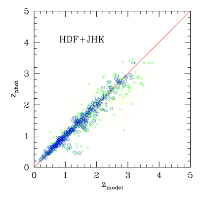
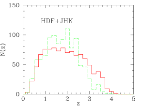
In the case of HDF-N filter set, we considered also two subcatalogues built with more restrictive selection criteria, requiring the detection both in $I_{814}$ and in at least two other filters to be $S/N\geq 5$ and $S/N\geq 10$. Statistics concerning these simulations are tabulated in Table 5. Obviously, when considering objects with increasing $S/N$, the accuracy of $z_{\rm phot}$ estimate significantly improves. In Figure 9 we show the results obtained on the comparison between $z_{\rm phot}$ and model redshifts, and also on the $N(z_{\rm model})$ versus $N(z_{\rm phot})$ reconstruction. Most of the discrepancy is due to objects with $S/N\leq 10$.

5.2 Shallow wide field surveys

Figure 10: Top: comparison between $z_{\rm model}$ and $z_{\rm phot}$ for realistic catalogue for a shallow survey with 5 filters. The symbols are the same as in Figure 9. Bottom: redshift distributions for the simulation on the top with $(S/N)_{\rm lim}=1$. Solid line: $N(z_{\rm model})$. Dashed line: $N(z_{\rm phot})$.

Figure 11: Top: comparison between $z_{\rm model}$ and $z_{\rm phot}$ for realistic catalogue for a shallow survey with 7 filters. The symbols are the same as in Figure 9. Bottom: redshift distributions for the simulation on the top with $(S/N)_{\rm lim}=1$. Solid line: $N(z_{\rm model})$. Dashed line: $N(z_{\rm phot})$.

$z=0.0$ – 0.4

0.4 – 1.0

1.0 – 2.0

2.0 – 3.0

$>3$

filters

$\sigma_{z}$

$l$%

$g$%

$\sigma_{z}$

$l$%

$g$%

$\sigma_{z}$

$l$%

$g$%

$\sigma_{z}$

$l$%

$g$%

$\sigma_{z}$

$l$%

$g$%

HDF+JHK

0.06

$0\pm 0$

$3\pm 7$

0.17

$1\pm 1$

$8\pm 3$

0.29

$1\pm 1$

$12\pm 2$

0.39

$8\pm 1$

$4\pm 1$

0.34

$30\pm 3$

$1\pm 1$

$S/N=5$

0.06

$0\pm 0$

$3\pm 7$

0.09

$0\pm 0$

$8\pm 2$

0.20

$0\pm 0$

$4\pm 2$

0.30

$1\pm 1$

$0\pm 1$

0.30

$2\pm 2$

$0\pm 0$

$S/N=10$

0.06

$0\pm 0$

$3\pm 7$

0.07

$0\pm 0$

$4\pm 2$

0.15

$0\pm 0$

$2\pm 1$

0.20

$0\pm 0$

$0\pm 0$

0.19

$0\pm 0$

$0\pm 0$

BVRI

(d)

0.08

$10\pm 8$

$38\pm 15$

0.32

$8\pm 2$

$40\pm 4$

0.46

$19\pm 1$

$10\pm 2$

0.56

$34\pm 3$

$4\pm 1$

0.47

$31\pm 6$

$7\pm 1$

(s)

0.17

$30\pm 3$

$10\pm 2$

0.36

$11\pm 2$

$7\pm 1$

0.45

$18\pm 1$

$6\pm 1$

0.70

$58\pm 7$

$32\pm 6$

—

—

—

UBVRI

(d)

0.06

$0\pm 0$

$37\pm 13$

0.30

$7\pm 1$

$21\pm 4$

0.43

$12\pm 2$

$10\pm 2$

0.50

$17\pm 2$

$4\pm 1$

0.46

$28\pm 3$

$5\pm 1$

$S/N=1$

(s)

0.15

$17\pm 1$

$25\pm 3$

0.34

$7\pm 1$

$4\pm 1$

0.49

$19\pm 2$

$2\pm 1$

0.58

$41\pm 10$

$14\pm 7$

—

—

—

$S/N=5$

(s)

0.09

$5\pm 1$

$7\pm 2$

0.26

$2\pm 1$

$2\pm 1$

0.49

$14\pm 6$

$2\pm 1$

—

—

—

—

—

—

$S/N=10$

(s)

0.07

$1\pm 1$

$2\pm 2$

0.18

$1\pm 1$

$1\pm 1$

0.43

$4\pm 7$

$4\pm 5$

—

—

—

—

—

—

UBVRIZ

(d)

0.06

$0\pm 0$

$20\pm 10$

0.23

$6\pm 2$

$28\pm 3$

0.45

$12\pm 2$

$2\pm 1$

0.43

$12\pm 2$

$11\pm 1$

0.48

$24\pm 2$

$6\pm 2$

(s)

0.14

$18\pm 1$

$25\pm 2$

0.29

$11\pm 1$

$7\pm 1$

0.53

$21\pm 2$

$1\pm 1$

0.42

$41\pm 9$

$35\pm 8$

—

—

—

UBVRIJ

(d)

0.05

$0\pm 0$

$13\pm 9$

0.19

$3\pm 1$

$25\pm 3$

0.37

$5\pm 1$

$6\pm 1$

0.42

$15\pm 2$

$6\pm 2$

0.43

$28\pm 3$

$2\pm 2$

(s)

0.17

$11\pm 1$

$19\pm 2$

0.25

$5\pm 1$

$4\pm 1$

0.45

$11\pm 2$

$2\pm 1$

0.50

$35\pm 8$

$28\pm 7$

—

—

—

UBVRIK

(d)

0.06

$0\pm 0$

$9\pm 11$

0.19

$3\pm 1$

$22\pm 2$

0.36

$5\pm 1$

$7\pm 1$

0.44

$14\pm 1$

$2\pm 1$

0.39

$14\pm 3$

$3\pm 2$

(s)

0.17

$14\pm 1$

$14\pm 2$

0.25

$7\pm 1$

$4\pm 1$

0.43

$11\pm 2$

$2\pm 1$

0.54

$34\pm 6$

$25\pm 7$

—

—

—

BVRIJK

(d)

0.06

$0\pm 0$

$7\pm 6$

0.17

$3\pm 1$

$32\pm 3$

0.39

$5\pm 2$

$9\pm 1$

0.43

$25\pm 3$

$4\pm 1$

0.40

$29\pm 2$

$3\pm 3$

(s)

0.19

$17\pm 2$

$6\pm 2$

0.24

$7\pm 1$

$2\pm 1$

0.39

$8\pm 1$

$4\pm 1$

0.37

$30\pm 6$

$58\pm 8$

—

—

—

UBVRIJK

(d)

0.06

$0\pm 0$

$5\pm 5$

0.17

$3\pm 1$

$23\pm 4$

0.35

$3\pm 1$

$8\pm 1$

0.41

$13\pm 3$

$4\pm 1$

0.38

$26\pm 4$

$2\pm 2$

$S/N=1$

(s)

0.17

$13\pm 2$

$12\pm 3$

0.24

$6\pm 1$

$3\pm 1$

0.40

$6\pm 2$

$3\pm 1$

0.43

$29\pm 7$

$34\pm 9$

—

—

—

$S/N=5$

(s)

0.09

$2\pm 1$

$6\pm 2$

0.15

$1\pm 1$

$3\pm 1$

0.40

$8\pm 2$

$2\pm 1$

—

—

—

—

—

—

$S/N=10$

(s)

0.06

$0\pm 0$

$2\pm 2$

0.11

$0\pm 0$

$2\pm 1$

0.27

$7\pm 10$

$5\pm 4$

—

—

—

—

—

—

UBVRI

(d)

0.05

$0\pm 0$

$5\pm 6$

0.17

$3\pm 1$

$24\pm 2$

0.35

$3\pm 1$

$8\pm 1$

0.39

$13\pm 2$

$6\pm 1$

0.38

$27\pm 3$

$2\pm 1$

JHK

(s)

0.17

$13\pm 2$

$9\pm 2$

0.24

$5\pm 1$

$3\pm 1$

0.38

$5\pm 1$

$4\pm 1$

0.36

$23\pm 4$

$41\pm 8$

—

—

—

Table 5: The dispersion $\sigma_{z}$ and the percentage of catastrophic and spurious objects, $l$% and $g$%, with errors, in five redshift bins, computed from 10 realizations of simulated catalogues with a redshift distribution derived from a PLE model. (s) and (d) refer to shallow and deep surveys respectively. The data are replaced by a dash when there are no enough data to compute the statistics. For the three examples in Figures 9, 10 and  11 we also present the quantities mentioned above as a function of the limiting signal to noise ratio considered for the detection.

In the second case, the aim is to reproduce the observational conditions reached when using 8 m telescopes and a wide field detector. In particular, we consider the case of a survey in a $\sim 60$ arcmin² field, observed with all the filter sets considered in Section 3. The adopted limiting magnitudes are shallower and conservative with respect to the values in the previous simulations. They are shown in the column $m_{\rm lim}$(s) of Table 4. The percentages of the different spectral types for catalogues with these limiting magnitudes, using the same detection criteria, are similar to the previous ones, being $\sim 12,54,26,8$% for E, Sb, Im, and Im(${\rm age}=0.1$ Gyr) respectively.

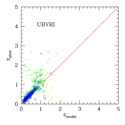
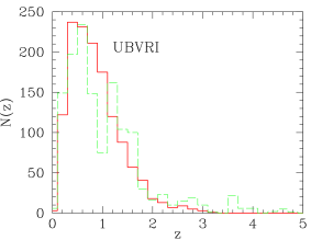
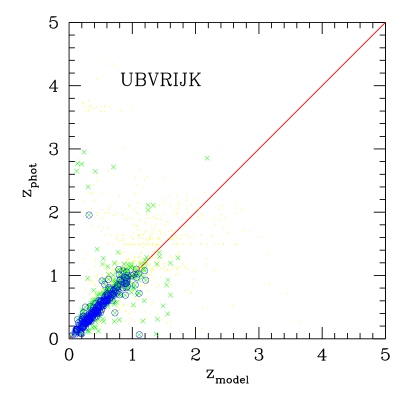
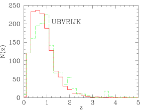
Results for $\sigma_{z}$, $l$% and $g$% are presented in Table 5 and marked by a (s). For the filter sets UBVRI and UBVRIJK we repeated the same procedure adopted for the HDF-N simulated catalogue, to build two subcatalogues with higher $S/N$ thresholds. Figure 10 presents the results obtained with the five optical bands only, whereas Figure 11 displays the equivalent results with the additional photometry in two near infrared filters. Figures 10 and 11 show the associated input and recovered redshift distributions.

The peak of the redshift distribution in this case is at a lower redshift compared to the HDF simulation. Wide-field surveys allow to obtain a better sampling of the bright end of the luminosity function with respect to HDF-like surveys, the later being more suited to explore the faint luminosity regime. The value of $g$% and $l$% change significantly when considering the same set of filters, but a different kind of survey. On the contrary, $\sigma_{z}$ remains similar.

An interesting feature is the opposite trend displayed by deep pencil-beam compared to shallow wide-field surveys with respect to the low and high redshift regimes for a given filter set. At low redshifts, the value of $g$% is larger for the deep pencil-beam survey (type (d) in the Table 5) than for the shallow (s) wide-field one. Conversely, the accuracy of deep surveys overcome that of the shallow ones at high redshifts. In this context, the separation between low and high redshift regimes is marked by the $z=1$ – $2$ bin.

This behaviour could be easily explained when we consider the different characteristics of the catalogues produced in the two cases. The deep survey catalogue contains few low redshift galaxies, and most of them derive from the faint tail of the luminosity function. These faint galaxies are much more abundant than the bright ones, than they are present in the catalogue even though the volume covered at low redshift by this survey is small. The photometric errors for these intrinsically faint objects are rather large, thus causing a poor estimate of $z_{\rm phot}$. On the contrary, the wide-field survey contains a large quantity of bright galaxies at low redshift, wich have sufficiently small photometric errors to obtain accurate $z_{\rm phot}$s. The faintest objects are lost in this case because of the shallow detection limits. The majority of galaxies in the shallow wide survey lies in the low redshift bins, around the peak of $N(z)$. When we consider the population of galaxies beyond the peak of the redshift distribution, the photometric errors in the shallow survey become important and an increasing fraction of objects is non detected in various filters. These problems hamper a robust determination of $z_{\rm phot}$. On the contrary, the pencil beam survey take advantage of its depth, allowing to compute $z_{\rm phot}$ at higher redshifts.

On the basis of these results, we caution that the kind of analysis presented here is strongly advised when a photometric survey is undertaken in view of computing $z_{\rm phot}$s. In particular, the filter configuration and the photometric depth to reach in each filter have to be determined accurately in advance, in order to optimize the survey and to study the feasibility of the project.

6 Discussion

Making use of the Bayesian technique, Benítez (2000) demonstrated that the dispersion of $z_{\rm phot}$ can be significantly improved. Despite of this result, we decide not to introduce this possibility in our code, at least for general purposes. The reason for this is that we want to prevent spurious effects in particular studies. As an example, when the luminosity function is imposed, the study of the galaxy population is constrained and it becomes impossible to obtain independent information on the properties of objects, thus limiting the possible applications. However, this method can be regarded with interest when the purpose is addressed to some specific application or when one is dealing with poor data, in such a way that the introduction of hints permits to obtain useful results. Alternatively, the photometric redshift estimate can be safely improved introducing the Bayesian inference when prior information is not related to photometric properties of sources. Examples of such priors that could be combined with the $z_{\rm phot}$ technique are the morphology or the clues inferred from gravitational lensing modeling.

One of the main issues for $z_{\rm phot}$ is the optimization of the visible versus near-IR bands for spectroscopic surveys. The aim is to produce a criterion based in $z_{\rm phot}$ to discriminate between objects showing strong spectral features in the optical and in the near-IR. To perform this test, both the redshift and the SED characteristics have to be estimated for each object. The $z_{\rm phot}$ and the SED are obtained by means of hyperz, together with the best fit parameters ($A_{V}$, spectral type, metallicity and age). The relevant information shall be the redshift and the rough SED type, i.e. “blue” or “red” continuum at the given $z$. We have shown that only limited information could be obtained on the parameter space from broad-band photometry alone. This situation will change with the future cryogenic imaging spectrophotometers, as presented in a recent paper by Mazin & Brunner (2000), because such devices will be able to gain in spectral resolution while spanning a large wavelength domain.

Another important issue for $z_{\rm phot}$ is the improvement on the cluster detection in wide-field photometric surveys. Including such a technique in an automated identification algorithm, whatever this algorithm is, allows to improve significantly the detection levels. The main idea is that the contrast between the cluster and the foreground and background population is the leading factor. When introducing a simple detection scheme, similar to the one used by Cappi et al. (1989), it is easy to quantify this effect (Pelló et al. 1998). In general, the $S/N$ is expected to improve by a factor of at least $\sim 2$ to $3$ with respect to the pure 2D case, depending on the cluster redshift and richness, the set of filters used and the depth of the survey. When considering more elaborated cluster-finding algorithms, such as the one produced by Kepner et al. (1999), Olsen et al. (1999), Scodeggio et al. (1999), Kawasaki et al. (1998) or Deltorn et al. (2000, in preparation), these results could be regarded as the relative improvement due to photometric redshifts. The present version of hyperz is also able to display the probability of each object to be at a fixed redshift. This is useful when looking for clusters of galaxies at a given (guessed) redshift.

The study of clustering properties through the spatial correlation function of galaxies, using the angular correlation together with the $z_{\rm phot}$ information is another possible application of $z_{\rm phot}$, aiming to extend the study of galaxy properties to fainter limits in magnitude. In this case, the relatively high number of objects accessible to photometry per redshift bin, suitably defined according to photometric redshift accuracy, allows to enlarge the spectroscopic sample towards the faintest magnitudes, and also to strongly reduce the errors (because the number of objects per redshift bin strongly increases). Studies on the evolution of the angular correlation function of galaxies in the HDF-N applying the photometric redshift technique can be found in Miralles & Pelló (1998), Connolly et al. (1998), Roukema et al. (1999), Arnouts et al. (1999), Magliocchetti & Maddox (1999), .

The same slicing procedure can be adopted to study the evolution of the luminosity function and consequently to infer the star formation history at high redshift from the UV luminosity density, as well as to analyse the stellar population and the evolutionary properties of distant galaxies (e.g. Yee et al. 1996, SubbaRao et al. 1996, Gwyn & Hartwick 1996, Sawicki et al. 1997, Connolly et al. 1997, Pascarelle et al. 1998, Giallongo et al. 1998).

Furthermore, the photometric redshift method has been used to investigate the nature of Extremely Red Objects (EROs) with a “spectro-photometric” technique by Cimatti et al. (2000), deducing clues about the model of galaxy formation. Another kind of spectroscopic and photometric combination has led to the identification of very high redshift object, as described by Chen et al. (1999).

From this not exhaustive list of applications, it is evident that photometric redshifts are a powerful and promising tool in many areas of extragalactic research. This method shall not be regarded only as a “poor person’s redshift machine”, but as a fundamental instrument, since a multitude of faint objects will remain beyond the limits of spectroscopy for the next years. Even with the diffusion of Multi-Object Spectrometers, most of the faint galaxies with measured photometry will fall beyond the reach of conventional spectroscopy.

7 Conclusions

We have presented the characteristics and the performances of our public code hyperz, available on the web, which make use of the template SED fitting technique. We can summarize the main conclusions as follows:

1. Simulations of ideal catalogues have shown the main trends of the accuracy on $z_{\rm phot}$ calculations. In particular, $z_{\rm phot}$ estimates are improved when the filters set spans a wide wavelength range, including near-IR and $U$ filters, and when the photometric errors become small.

2. We have investigated the weight of the different parameters on the final results, using both a spectroscopic subsample of HDF and simulations. In particular, the templates, the flux decrement by Lyman forest, the age of the stellar population, the reddening, the cosmology, the metallicity, the IMF and the presence of emission lines have been discussed. According to these results, the $z_{\rm phot}$ preciseness seems to be more sensitive to the photometric accuracy rather than to the detailed set of parameters. Nevertheless, a subset of these parameters (reddening, age of the stellar population and Lyman forest blanketing) has to span a sufficiently wide range of values to obtain accurate $z_{\rm phot}$s.

3. The robustness of the method has been illustrated through realistic deep field simulations, aiming to reproduce the redshift distribution, photometric accuracy and limiting magnitudes encountered in deep field surveys.

4. We have pointed out some of the manifold applications of the photometric redshift machinery in present and future projects.

5. We plan to include AGN SEDs in the present scheme of hyperz, as well as stellar templates, in order to automatically classify objects in a photometric survey through a unique pipeline. This particular application is presently under development (Hatziminaoglou et al. 2000).