Large-Scale Sunyaev-Zel’dovich Effect: Measuring Statistical Properties with Multifrequency Maps

Abstract

We study the prospects for extracting detailed statistical properties of the Sunyaev-Zel’dovich (SZ) effect associated with large scale structure using upcoming multifrequency CMB experiments. The greatest obstacle to detecting the large-angle signal is the confusion noise provided by the primary anisotropies themselves, and to a lesser degree galactic and extragalactic foregrounds. We employ multifrequency subtraction techniques and the latest foregrounds models to determine the detection threshold for the Boomerang, MAP (several $\mu$K) and Planck CMB (sub $\mu$K) experiments. Calibrating a simplified biased-tracer model of the gas pressure off recent hydrodynamic simulations, we estimate the SZ power spectrum, skewness and bispectrum through analytic scalings and N-body simulations of the dark matter. We show that the Planck satellite should be able to measure the SZ effect with sufficient precision to determine its power spectrum and higher order correlations, e.g. the skewness and bispectrum. Planck should also be able to detect the cross correlation between the SZ and gravitational lensing effect in the CMB. Detection of these effects will help determine the properties of the as yet undetected gas, including the manner in which the gas pressure traces the dark matter.

1. Introduction

It is by now well established that the precision measurements of the cosmic microwave background expected from upcoming experiments, especially MAP and Planck satellite missions, will provide a gold mine of information about the early universe and the fundamental cosmological parameters (e.g., Jungman et al. 1996). These experiments can in fact do so much more. With all-sky maps across the wide range of uncharted frequencies from $20$GHz-$900$GHz, the secondary science from these missions will arguably be as interesting as the primary science.

In this paper, we examine the prospects for extracting the large-scale properties of the hot intergalactic gas from multifrequency observations of the CMB. Inverse-Compton scattering of CMB photons by hot gas, known as the Sunyaev-Zel’dovich (SZ; Sunyaev & Zel’dovich 1980) effect, leaves a characteristic distortion in the spectrum of the CMB, which fluctuates in the sky with the gas density and temperature. In the Rayleigh-Jeans (RJ) regime, it produces a constant decrement and with only low frequency measurements, the much larger primary anisotropies in the CMB itself obscure the fluctuations on scales greater than a few arcminutes (e.g., Goldberg & Spergel 1999). The upscattering in frequency implies an increment at high frequencies and a null around $217$GHz. This behavior provides a potential tool for the separation of SZ effect from other temperature anisotropy contributors.

Since both the SZ spectrum and the CMB spectrum are accurately known, one can expect that foreground removal techniques developed to isolate the primary anisotropies can be reversed to recover the SZ signal in the presence of noise from the primary anisotropies. Galactic and extragalactic foregrounds will be more challenging to remove. Here we use the latest foreground models from Tegmark et al. (1999) that takes into account the fact that imperfect correlations in the foregrounds between frequency channels inhibits our ability to remove them. Using foreground information together with the expected noise properties of individual experiments, one can determine the minimal detectable signal in each experiment and the upper limit achievable in the absence of detection. Experiments with sufficient signal-to-noise can extract precision measurements for the power spectrum and higher order statistics such as the skewness. Ultimately, they can provide detailed maps of the large-angle SZ effect.

To assess the prospects for an actual detection, we must model the SZ signal itself. The SZ effect is now routinely imaged in massive galaxy clusters (e.g., Carlstrom et al 1996; Jones et al 1993), where the temperature of the scattering medium can reach as high as 10 keV, producing temperature changes in the CMB of order 1 mK at RJ wavelengths. The possibility for detection of massive clusters in CMB satellite data has already been discussed in several studies (e.g., Aghanim et al. , Haehnelt & Tegmark 1996, Pointecouteau et al 1998). Here, however, we are interested in the SZ effect produced by large-scale structure in the general intergalactic medium (IGM) where the gas is expected to be at $\lesssim 1$keV in mild overdensities, leading to CMB contributions in the $\mu$K range.

It is now widely believed that at least $\sim$ 50% of the present day baryons, when compared to the total baryon budget from big bang nucleosynthesis, are present in gas associated with hot large-scale structure which has remained undetected given its temperature and clustering properties (e.g., Fukugita et al 1998; Cen & Ostriker 1999; Pen 1999). Recently, Scharf et al (2000) has provided a tentative detection of X-ray emission from a large-scale filament in one of the deep ROSAT PSPC fields; previous attempts yielding upper limits are described in Kull & Böhringer (1999) and Briel & Henry (1995). These results are consistent with current predictions for the X-ray surface brightness based on numerical simulations (e.g., Cen et al 1995). Pen (1999) argued that non-gravitational heating of the gas to $\sim 1$keV is required to evade bounds from the soft X-ray background. These results suggest that the X-ray emission from this gas may be detectable in the near future with wide-field observations with Chandra X-ray Observatory and X-ray Multiple Mirror Mission.

On the theoretical front, hydrodynamic simulations of the SZ effect continue to improve (da Silva et al. 1999; Refregier et al. 1999; Seljak et al. 2000). As a consensus from these simulations of basic properties such as the opacity weighted gas temperature and average Compton distortion is still lacking, we will base our assessment of the detectability of the large-scale SZ effect on a simple parameterization of the effect, based on a gas pressure bias model (Refregier et al. 1999), crudely calibrated with the recent hydrodynamic simulations. We employ perturbation theory, non-linear scaling relations, and N-body simulations for the dark matter to assess the statistical properties of the signal. Properly calibrated, these techniques can complement hydrodynamic simulations by extending their dynamic range and sampling volume. Currently, they should simply be taken as order of magnitude estimates of the potential signal.

Throughout this paper, we will take an adiabatic cold dark matter (CDM) model as our fiducial cosmology. We assume cosmological parameters $\Omega_{c}=0.30$ for the cold dark matter density, $\Omega_{b}=0.05$ for the baryon density, $\Omega_{\Lambda}=0.65$ for the cosmological constant, $h=0.65$ for the dimensionless Hubble constant and a COBE-normalized scale invariant spectrum of primordial fluctuations (Bunn & White 1997).

The layout of the paper is as follows. In § 2, we describe the foreground and primary anisotropy removal method and assess their efficacy for upcoming CMB experiments. In § 3, we detail the bias model for the SZ effect and calculate through perturbation theory, analytic approximations and numerical simulations, the low order statistics of the SZ effect: its power spectrum, skewness and bispectrum. In § 4, having estimated the noise and the signal, we assess the prospects for measuring these low order statistics in upcoming experiments. We conclude in § 5 with a discussion of our results.

Figure 1.— Top: foreground contributions to temperature anisotropies $(\Delta T/T)^{2}=l(l+1)C_{l}/2\pi$ from the various foregrounds (dust, free-free, synchrotron, radio and infrared point sources, and rotating dust) at three fiducial frequencies as labeled. The SZ signal (solid, unlabeled) is estimated with the simplified model of § 3. Bottom: residual foregrounds after multifrequency subtraction for Boomerang, MAP and Planck. The total includes detector noise and residual CMB.

2. Modeling the CMB and Foreground Noise

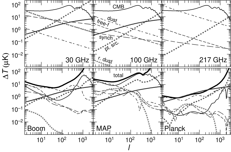
The main obstacle for the detection of the SZ effect from large-scale structure for angular scales above a few arcminutes is the CMB itself. Here the primary anisotropies dominate the SZ effect for frequencies near and below the peak in the CMB spectrum (see Fig. 1). Fortunately, the known frequency dependence and statistical properties of primary anisotropies allows for extremely effective subtraction of their contribution (e.g., Hobson et al 1998; Bouchet & Gispert 1999). In particular, primary anisotropies obey Gaussian statistics and follow the blackbody spectrum precisely.

Perhaps more worrying are the galactic and extragalactic foregrounds, some of which are expected to to be at least comparable to the SZ signal in each frequency band. These foregrounds typically have spatial and/or temporal variations in their frequency dependence leading to imperfect correlations between their contributions in different frequency bands. We attempt here to provide as realistic an estimate as possible of the prospects for CMB and foreground removal, given our incomplete understanding of the foregrounds.

Table 1

CMB Experimental Specifications Experiment $\nu$ FWHM $10^{6}\Delta T/T$ Boomerang 90 20 7.4 150 12 5.7 240 12 10 400 12 80 MAP 22 56 4.1 30 41 5.7 40 28 8.2 60 21 11.0 90 13 18.3 Planck 30 33 1.6 44 23 2.4 70 14 3.6 100 10 4.3 100 10.7 1.7 143 8.0 2.0 217 5.5 4.3 353 5.0 14.4 545 5.0 147 857 5.0 6670

NOTES.—Specifications used for Boomerang, MAP and Planck. Full width at half maxima (FWHM) of the beams are in arcminutes and should be converted to radians for the noise formula. Boomerang covers a fraction $\sim$ 2.6% of the sky, while we assume a usable fraction of 65% for MAP and Planck. In § 4, in order to calculate the maximum signal-to-noise, we define a perfect experiment as one with no instrumental noise and full sky coverage.

2.1. Foreground Model and Removal

We use the “MID” foreground model of Tegmark et al. (1999) and adapt the subtraction techniques found there for the purpose of extracting the SZ signal. The assumed level of the foreground signal in the power spectrum for three fiducial frequencies is shown in Fig. 1.

The foreground model is defined in terms of the covariance between the multipole moments at different frequency bands

$$\left<a_{l^{\prime}m^{\prime}}^{{\rm f}*}(\nu^{\prime})a_{lm}^{{\rm f}}(\nu)\right>=C_{l}^{{\rm f}}(\nu^{\prime},\nu)\delta_{ll^{\prime}}\delta_{mm^{\prime}}\,,$$ (1)

in thermodynamic temperature units as set by the CMB blackbody. In this section, we will speak of the primary anisotropies and detector noise simply as other foregrounds with very special properties:

$$C_{l}^{\rm CMB}(\nu^{\prime},\nu) = C_{l}\,,$$

$$C_{l}^{\rm noise}(\nu^{\prime},\nu) = 8\ln 2\theta(\nu)^{2}e^{\theta^{2}(\nu)l(l+1)}\left({\Delta T\over T}\right)^{2}\Big{|}_{\rm noise}\delta_{\nu,\nu^{\prime}}\,.$$

The FWHM$=\sqrt{8\ln 2}\theta$ and noise specifications of the Boomerang, MAP and Planck frequency channels are given in Tab. 1. True foregrounds generally fall in between these extremes of perfect and no frequency correlation.

The difference between extracting the SZ signal and the primary signal is simply that one performs the subtraction referenced to the SZ frequency dependence

$$s(\nu)=2-{x\over 2}\coth{x\over 2}\,,$$ (3)

where $x=h\nu/kT_{\rm cmb}\approx\nu/56.8$GHz. Note that in the RJ limit $s(\nu)\rightarrow 1$ such that

$$C_{l}^{\rm SZ}(\nu,\nu^{\prime})=s(\nu)s(\nu^{\prime})C_{l}^{\rm SZ}$$ (4)

where $C_{l}^{\rm SZ}$ is the SZ power spectrum in the RJ limit.

Consider an arbitrary linear combination of the channels,

$$b=\sum_{\nu_{i}}{1\over s(\nu_{i})}w(\nu_{i})a(\nu_{i})\,.$$ (5)

Since the subtraction is done multipole by multipole, we have temporarily suppressed the multipole index. The covariance of this quantity is

$$\left<b^{2}\right>=C^{{\rm SZ}}[\sum_{\nu_{i}}w(\nu_{i})]^{2}+\sum_{\nu_{i},\nu_{j}}w(\nu_{i})w(\nu_{j})\sum_{{\rm f}}{C^{\rm f}(\nu_{i},\nu_{j})\over s(\nu_{i})s(\nu_{j})}\,.$$ (6)

Minimizing the variance contributed by the foregrounds subject to the constraint that the SZ estimation be unbiased, we obtain

$$\sum_{\nu_{i}}w(\nu_{j})\sum_{{\rm f}}{C^{\rm f}(\nu_{i},\nu_{j})\over s(\nu_{i})s(\nu_{j})}={\rm const.}\,$$ (7)

Defining the scaled foreground covariance matrix as

$$\tilde{C}(\nu_{i},\nu_{j}) = \sum_{{\rm f}}{C^{\rm f}(\nu_{i},\nu_{j})\over s(\nu_{i})s(\nu_{j})},$$ (8)

$$\equiv \sum_{{\rm f}}\tilde{C}^{\rm f}(\nu_{i},\nu_{j})\,,$$

we solve for the weights that minimize the noise variance

$${\bf w}\propto{\tilde{\bf C}^{-1}{\bf e}}\,,$$ (9)

where ${\bf e}$ is the vector of all ones $e(\nu_{i})=1$. Finally we normalize the sum of the weights to unity $\sum w(\nu_{i})=1$ to obtain an unbiased estimator. Our approach is same as minimizing the foreground variance subject to the constraint that the recovered multipole is an unbiased estimate of the true SZ signal. As each channel is rescaled such that SZ signal corresponds to the RJ level, the weights sum to unity.

The total residual noise variance in the map from the foregrounds per multipole is then

$$N_{l}={\bf w}_{l}^{t}{\tilde{\bf C}_{l}}{\bf w}_{l}\,,$$ (10)

and from each foreground component

$$N_{l}^{\rm f}={\bf w}_{l}^{t}{\tilde{\bf C}_{l}^{\rm f}}{\bf w}_{l}\,.$$ (11)

Note that the residual noise in the map is independent of assumptions about the SZ signal including whether it is Gaussian or not. However if the foregrounds themselves are non-Gaussian, then this technique only minimizes the variance and may not be optimal for recovery of non-Gaussian features in the SZ map itself. Bouchet et al (1995) have shown that similar techniques are quite effective even when confronted with non-Gaussian foregrounds. This is a potential caveat especially for cases in which the residual noise is not dominated by the primary anisotropies or detector noise. We shall discuss methods to alleviate this concern in the next section.

Figure 2.— Dependence of the residual noise rms on foreground assumptions expressed as a ratio to the fiducial model of Fig. 1. (a) Falsely assuming the foregrounds have perfect frequency coherence not only underpredicts the residual noise by a substantial factor but also leads to substantially more actual residual noise. (b) Multiplying the foreground amplitudes by 2 (power by 4) produces less than a factor of 2 increase in the residual noise.

2.2. Detection Threshold

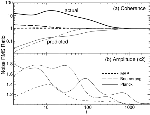
The residual noise sets the detection threshold for the SZ effect for a given experiment. In Fig. 1, we show the rms of the residual noise after foreground subtraction for the Boomerang, MAP and Planck experiments assuming the “MID” foreground model from Tegmark et al. (1999). With the Boomerang and Planck channels, elimination of the primary anisotropies is excellent up to the beam scale where detector noise dominates. As expected, the MAP channels, which are all on the RJ side of the spectrum, do not allow good elimination of the primary anisotropies.

It is important not to assume that the foregrounds are perfectly correlated in frequency, which is the usual assumption in the literature (Hobson et al 1998; Bouchet & Gispert 1999). There are two types of errors incurred by doing so. The first is that one underpredicts the amount of residual noise in the SZ map (see Fig. 2). The second is that if one calculates the optimal weights in equation (9) based on this assumption the actual residual noise increases. For Planck it can actually increase the noise beyond the level in which it appears in the $100$GHz maps with no foreground subtraction at all. The reason is that the cleaning algorithm then erroneously uses the contaminated high and low frequency channels to subtract out the small foreground contamination in the central channels. In Planck, the difference between the predicted and actual rms noise from falsely assuming perfect frequency coherence can be more than two orders of magnitude.

For Boomerang and Planck, the largest residual noise component, aside from detector noise, is dust emission and is sufficiently large that one might worry that current uncertainties in our knowledge of the foreground model may affect the implications for the detection of the SZ effect. It is therefore important to explore variations on our fiducial foreground model.

Multiplying the foreground rms amplitudes uniformly by a factor of 2 (and hence the power by a factor of 4), produces less than a factor of 2 increase in the residual noise rms as shown in Fig. 2. Likewise, as discussed in Tegmark et al. (1999), minor variations in the frequency coherence do not effect the residual noise much in spite of the fact that it is crucial not to assume perfect correlation. We conclude that uncertainties in the properties of currently known foregrounds are unlikely to change our conclusions qualitatively. There is however always the possibility that some foreground that does not appear in the currently-measured frequency bands will affect our results.

The fact that the residual dust contributions are comparable to those of the detector noise for Boomerang and Planck is problematic for another reason. Since the algorithm minimizes to total residual variance, it attempts to keep these two main contributors roughly comparable. However the dust will clearly be non-Gaussian to some extent and one may prefer instead to trade more residual detector noise for dust contamination. One can modify the subtraction algorithm to account for this by artificially increasing the rms amplitude of the dust when calculating the weights in equation (9) while using the real amplitude in calculating the residual noise in equation (11). For example we have explored increasing the amplitude by a factor of 4 (power by 16) for the weights. The result is an almost negligible increase in total residual noise rms but an improvement in dust rejection by a factor of 3-4 in rms. For Planck this brings the ratio of dust to total rms to $\sim 10\%$ and recall that the noise adds in quadrature so that the total dust contribution is really $\sim 1\%$ of the total. This more conservative approach is thus advisable but since it leaves the total residual noise rms essentially unchanged, we will adopt the minimum variance noise to estimate the detection threshold.

Fig. 1 directly tells us the detection threshold per $(l,m)$ multipole moment. Since the SZ signal is likely to have a smooth power spectrum in $l$, one can average over bands in $l$ to beat down the residual noise. Assuming Gaussian-statistics, the residual noise variance $2N_{l}^{2}$ for the power spectrum estimate is then given by

$$N_{l}^{-2}\Big{|}_{\rm band}={f_{\rm sky}}\sum_{l_{\rm band}}(2l+1)N_{l}^{-2}\,,$$ (12)

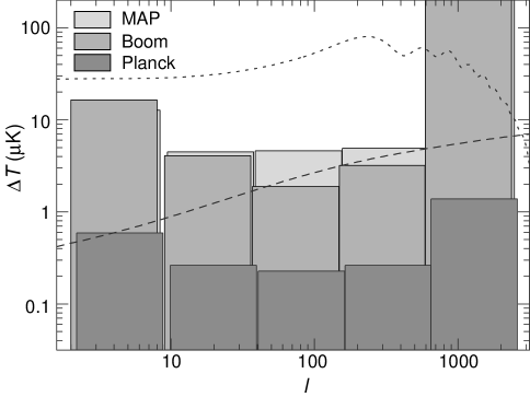
where $f_{\rm sky}$ accounts for the reduction of the number of independent modes due to the fraction of sky covered. The result for the three experiments is shown in Fig. 3. In the absence of a detection, they can be interpreted as the optimal 1 $\sigma$ upper limits on SZ bandpowers achievable by the experiment. Boomerang and MAP can place upper limits on the SZ signal in the interesting $\mu$K regime whereas Planck can detect signals well below a $\mu$K.

This noise averaging procedure in principle implicitly assumes that the statistical properties of the residual noise, and by implication the full covariance matrix of the other foregrounds, is precisely known. In reality, they too must be estimated from the multifrequency data itself through either through the subtraction techniques discussed here or by direct modeling of the foregrounds in the maps. Tegmark et al. (1999) found that direct modeling of the foregrounds with hundreds of fitted parameters did not appreciably degrade our ability to extract the properties of the primary anisotropies. The main source of variance there was the cosmic variance of the primary anisotropies themselves whose properties are precisely known. Similarly here the main source of residual variance is either the primary anisotropies (for MAP) or detector noise (for Boomerang and Planck) and their statistical properties may safely be considered known.

Figure 3.— Detection thresholds for the SZ effect. Error boxes represent the 1-$\sigma$ rms residual noise in multipole bands and can be interpreted as the detection threshold. Also shown (dotted) is the level of the primary anisotropies that have been subtracted with the technique and the signal (dashed) expected in the simplified model of §3.

3. Modeling the SZ Signal

In order to estimate how well the statistical properties of the SZ effect might be recovered with multifrequency CMB maps, we need to model the large-angle SZ effect itself. The current state-of-the-art in hydrodynamic simulations (da Silva et al. 1999; Refregier et al. 1999; Seljak et al. 2000) has reached a qualitative but not quantitative consensus on the statistical properties of the SZ effect. In addition, questions as to the heating of the gas from non-gravitational sources may even change the results qualitatively (Pen 1999). Hydrodynamic simulations are also severely limited in the dynamic range and volume sampled.

Given the current state of affairs, we believe it is useful to explore a parameterized model of the effect whose consequences are simple to calculate and which may be calibrated against hydrodynamic simulations as they continue to improve.

3.1. Bias Prescription

In general, the SZ temperature fluctuation $\Theta=\Delta T/T$ is given by the opacity weighted integrated pressure fluctuation along the line of sight:

$$\Theta^{\rm SZ}(\hat{\bf n},\nu) = -2s(\nu)\int_{0}^{r_{0}}dr\ \dot{\tau}\pi(r,\hat{\bf n}r)\,,$$ (13)

$r$ is the the comoving distance, $\tau$ is the Thomson optical depth, overdots are derivatives with respect to $r$ and the dimensionless electron pressure fluctuation is

$$\pi=\delta p_{e}/\rho_{e}\,.$$ (14)

One needs to model the statistical properties of $\pi$, in particular its power spectrum and bispectrum

$$\left<\pi({\bf k})^{*}\pi({\bf k}^{\prime})\right> = (2\pi)^{3}\delta^{\rm D}({\bf k}-{\bf k}^{\prime})P_{\pi}(k)\,,$$ (15)

$$\left<\pi({\bf k})\pi({\bf k}^{\prime})\pi({\bf k}^{\prime\prime})\right> = (2\pi)^{3}\delta^{\rm D}({\bf k}+{\bf k}^{\prime}+{\bf k}^{\prime\prime})B_{\pi}(k,k^{\prime},k^{\prime\prime})\,,$$

as a function of lookback time or distance $r$. In principle we also need the unequal time correlators, but in practice these do not play a role as we shall see.

By analogy to the familiar case of galaxy clustering, it is reasonable to suppose that the pressure fluctuations depend locally on the dark matter density and hence are biased tracers of the dark matter density in the linear regime (Goldberg & Spergel 1999). Hence the statistical properties follow from those of the dark matter distribution

$$P_{\pi}(k;r) \approx b_{\pi}(r)^{2}P_{\delta}(k;r)\,,$$

$$B_{\pi}(k,k^{\prime},k^{\prime\prime};r) \approx b_{\pi}(r)^{3}B_{\delta}(k,k^{\prime},k^{\prime\prime};r)\,.$$ (16)

We have restored the time dependence since the bias will be time dependent even in the linear regime and must be extracted from simulations. In general, the bias parameter for the power spectrum and bispectrum need not be the same even in the linear regime since the bispectrum automatically involves higher order corrections (Fry & Gaztanaga 1993). For estimation purposes here we will take them to be equal.

Following Goldberg & Spergel (1999), we chose the form

$$b_{\pi}(r)=b_{\pi}(0)/(1+z)\,,$$ (17)

as motivated by findings that the average gas temperature drops off roughly by this factor. We normalize the value of the bias parameter today by comparison with recent hydrodynamic simulations. It is conceptually useful to separate the bias into two factors:

$$b_{\pi}(0)={k_{B}T_{e}(0)\over m_{e}c^{2}}b_{\delta}\,,$$ (18)

i.e. an opacity-weighted average temperature and a bias parameter for the gas density at that temperature. In Refregier et al. (1999), for our fiducial $\Lambda$CDM cosmology, the bias $b_{\delta}$ was found to be $\sim$ 8 to 9, while in Seljak et al. (2000) it was found to be in the range $\sim$ of $3$ to $4$. In both these papers, $T_{e}(0)\sim$ 0.3 to 0.4 keV; these values are lower than the $\sim$ 1 keV found by Cen & Ostriker (1999) using hydrodynamical simulations with feedback effects. As a compromise between these results, we take $T_{e}(0)=0.5$keV and $b_{\delta}=4$, which corresponds to

$$b_{\pi}(0)=0.0039\,.$$ (19)

Note that this is a factor of 2 lower than used in Goldberg & Spergel (1999) and Cooray & Hu (1999).

Needless to say, the resulting predictions should be taken as order-of-magnitude estimates only. As simulations improve, one can expect better values for the bias today and a more detailed modeling of its redshift and perhaps even scale dependence.

3.2. Multipole Moments

The multipole moments of the SZ effect under these simplifying assumptions can then be expressed as a weighted projection of the density field (Cooray & Hu 1999):

$$a_{lm}^{\rm SZ}(0) \equiv \int d\hat{\bf n}Y_{l}^{m*}(\hat{\bf n})\Theta^{\rm SZ}(\hat{\bf n},0)$$ (20)

$$\approx i^{l}\int{d^{3}{\bf k}\over 2\pi^{2}}\delta({\bf k},r_{l})I_{l}^{\rm SZ}(k)Y_{l}^{m}{}^{*}(\hat{\bf k})\,,$$

where

$$I_{l}^{\rm SZ}(k) \approx W^{{\rm SZ}}(r_{l})\sqrt{{\pi\over 2l}}{1\over k}F_{l}(k)\,,$$

$$W^{\rm SZ}(r) = -2b_{\pi}(r)\dot{\tau}\,,$$ (21)

in the Limber approximation and (Hu 2000a)

$$r_{l} = \Omega_{K}^{-1/2}H_{0}^{-1}\sinh^{-1}(\Omega_{K}^{1/2}H_{0}l/k)\,,$$

$$F_{l} = (1+\Omega_{K}H_{0}^{2}l^{2}/k^{2})^{-1/4}\,.$$ (22)

The quantities take on a simple forms for a flat universe: $r_{l}\rightarrow l/k$ and $F_{l}(k)\rightarrow 1$. The Limber approximation breaks down for $l\hbox{ \raise 1.50696pt\hbox to0.0pt{$<$\hss}\lower 2.58334pt\hbox{$\sim$}\ }50$ but is sufficient for our purposes.

Figure 4.— top: SZ power spectrum from simulations compared to analytical predictions based on linear perturbation theory (PT) and the non-linear scaling relations of Peacock & Dodds (1996; PD96). bottom: Errors on the binned power spectrum estimators for a single $6^{\circ}\times 6^{\circ}$ field; for a given experiment the errors should be scaled by $\sim 0.03f_{\rm sky}^{-1/2}$. The sampling errors in the simulations is nearly equal to those of a Gaussian random field with the same power spectrum. The total noise including residual foregrounds and detector noise is also given for Planck.

3.3. Power Spectrum

The power spectrum of the SZ effect in this simplified model follows from equation (20),

$$C_{l}^{{\rm SZ}} = {2\over\pi}\int{dk\over k}{k^{3}P_{\delta}\left(k;r_{l}\right)}[I_{l}^{\rm SZ}(k)]^{2}\,,$$ (23)

$$\approx \int_{0}^{r_{0}}dr{[W^{\rm SZ}(r)]^{2}\over d_{A}^{2}}P_{\delta}(l/d_{A};r)\,,$$

In the second line we have transformed the integration variable under the Limber correspondence: $k=l/d_{A}$ and

$$\int{dk\over k}F_{l}^{2}\ldots=\int{dr\over d_{A}}\ldots\;.$$ (24)

We see that to go from the flat to curved cosmologies in the Limber approximation one simply replaces the radial distance with the angular diameter distance in the integrand.

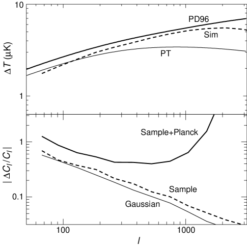
In evaluating the SZ power spectrum, we have extended the SZ model to the non-linear regime by using the scaling formulae for the nonlinear dark matter power spectrum of Peacock & Dodds (1996). However, modeling the SZ effect with a scale-independent bias factor will clearly break down deep in the non-linear regime. Refregier et al. (1999) have shown that it is a reasonable approximation in the weakly non-linear regime (overdensities $\hbox{ \raise 1.50696pt\hbox to0.0pt{$<$\hss}\lower 2.58334pt\hbox{$\sim$}\ }10$) for $z\hbox{ \raise 1.50696pt\hbox to0.0pt{$<$\hss}\lower 2.58334pt\hbox{$\sim$}\ }1$ but can be in serious error outside of this range. As the weakly non-linear regime is the one of interest for anisotropies at $l\hbox{ \raise 1.50696pt\hbox to0.0pt{$<$\hss}\lower 2.58334pt\hbox{$\sim$}\ }1000$, we will use this approximation to test the effects of non-linearities. The predicted power spectrum in our fiducial model is shown in Fig. 4.

3.4. Bispectrum

The bispectrum of the SZ effect also follows from expression (20)

$$B_{l_{1}l_{2}l_{3}}^{m_{1}m_{2}m_{3}} \equiv \left<a_{l_{1}m_{1}}a_{l_{2}m_{2}}a_{l_{3}m_{3}}\right>$$

$$= \left[\prod_{j=1}^{3}i^{l_{j}}\int\frac{d^{3}k_{j}}{2\pi^{2}}I_{l_{j}}^{\rm SZ}(k_{j})Y_{l}^{m\ast}(\hat{\bf k}_{j})\right]$$

$$(2\pi)^{3}\delta^{\rm D}({\bf k}_{1}+{\bf k}_{2}+{\bf k}_{3})B_{\delta}(k_{1},k_{2},k_{3})\,.$$

Here the density bispectrum should be understood as arising from the full unequal time correlator

$$\left<\delta({\bf k}_{1};r_{1})\delta({\bf k}_{2};r_{2})\delta({\bf k}_{3};r_{3})\right>\,,$$ (25)

where the temporal coordinate, which we temporarily suppress, is evaluated in the Limber approximation (22).

To further simplify this expression, we expand the delta function

$$\delta^{\rm D}({\bf k}_{1}+{\bf k}_{2}+{\bf k}_{3})=\frac{1}{(2\pi)^{3}}\int e^{i({\bf k}_{1}+{\bf k}_{2}+{\bf k}_{3})\cdot\hat{\bf n}r}d^{3}x\,,$$ (26)

and employ the Rayleigh expansion

$$e^{i{\bf k}\cdot\hat{\bf n}r}=4\pi\sum_{lm}i^{l}j_{l}(kr)Y_{l}^{m\ast}(\hat{{\bf k}})Y_{l}^{m}(\hat{\bf n})\,.$$ (27)

We have assumed here a flat universe to simplify the derivation; as we have seen in the last section, we can promote the final result to a curved universe by replacing radial distances with angular diameter distances.

With these relations, the angular integral over the directions of ${\bf k}_{j}$ collapse to give

$$B_{l_{1}l_{2}l_{3}}^{m_{1}m_{2}m_{3}} = \int r^{2}dr\left[\prod_{j=1}^{3}{2\over\pi}\int k_{j}^{2}dk_{j}I_{l_{j}}^{\rm SZ}(k_{j})j_{l_{j}}(k_{j}r)\right]$$ (28)

$$\times B(k_{1},k_{2},k_{3})G_{l_{1}l_{2}l_{3}}^{m_{1}m_{2}m_{3}}\,,$$

where the Gaunt integral is

$$G_{l_{1}l_{2}l_{3}}^{m_{1}m_{2}m_{3}} \equiv \int d\hat{\bf n}Y_{l_{1}}^{m_{1}}Y_{l_{2}}^{m_{2}}Y_{l_{3}}^{m_{3}}$$ (34)

$$= \sqrt{(2l_{1}+1)(2l_{2}+1)(2l_{3}+1)\over 4\pi}$$

$$\times\left(\begin{array}[]{ccc}l_{1}&l_{2}&l_{3}\\ 0&0&0\end{array}\right)\left(\begin{array}[]{ccc}l_{1}&l_{2}&l_{3}\\ m_{1}&m_{2}&m_{3}\end{array}\right)\,.$$

Here, the quantities in parentheses are the Wigner-3$j$ symbols whose properties are described in Appendix A of Cooray & Hu (1999). The integrals over the Bessel functions can again be done in the Limber approximation leaving

$$B_{l_{1}l_{2}l_{3}}^{m_{1}m_{2}m_{3}} = G_{l_{1}l_{2}l_{3}}^{m_{1}m_{2}m_{3}}\int dr{[W^{\rm SZ}(r)]^{3}\over r^{4}}B_{\delta}({l_{1}\over r},{l_{2}\over r},{l_{3}\over r};r)\,,$$

Note that only equal time contributions contribute in the Limber approximation.

We can promote this result to a curved universe by replacing radial distances with angular diameter distances

$$B_{l_{1}l_{2}l_{3}}^{m_{1}m_{2}m_{3}} = G_{l_{1}l_{2}l_{3}}^{m_{1}m_{2}m_{3}}\int dr{[W^{\rm SZ}(r)]^{3}\over d_{A}^{4}}B_{\delta}({l_{1}\over d_{A}},{l_{2}\over d_{A}},{l_{3}\over d_{A}};r)\,.$$

Finally, we can introduce the angular averaged bispectrum as

$$B_{l_{1}l_{2}l_{3}}=\sum_{m_{1}m_{2}m_{3}}\left(\begin{array}[]{ccc}l_{1}&l_{2}&l_{3}\\ m_{1}&m_{2}&m_{3}\end{array}\right)B_{l_{1}l_{2}l_{3}}^{m_{1}m_{2}m_{3}}\,,$$ (37)

to obtain the final result

$$B_{l_{1}l_{2}l_{3}} = \sqrt{(2l_{1}+1)(2l_{2}+1)(2l_{3}+1)\over 4\pi}\left(\begin{array}[]{ccc}l_{1}&l_{2}&l_{3}\\ 0&0&0\end{array}\right)$$ (41)

$$\times\int dr{[W^{\rm SZ}(r)]^{3}\over d_{A}^{4}}B_{\delta}({l_{1}\over d_{A}},{l_{2}\over d_{A}},{l_{3}\over d_{A}};r)\,.$$

One can alternately derive this relation by taking a flat-sky approach and using the general relation between the flat-sky and all-sky bispectra (see Appendix C, Hu 2000b).

Equation (41) gives the SZ angular bispectrum in terms of the underlying density bispectrum. In second order perturbation theory, the density bispectrum is in turn given by

$$B_{\delta}(k_{1},k_{2},k_{3};r) = F_{2}({\bf k}_{1},{\bf k}_{2})P_{\delta}(k_{1};r)P_{\delta}(k_{2};r)$$ (42)

$$+5\;{\rm perm.}\,,$$

where

$$F_{2}({\bf k}_{1},{\bf k}_{2})=\frac{5}{7}+\frac{{\bf k}_{1}\cdot{\bf k}_{2}}{k_{2}^{2}}+\frac{2}{7}\frac{({\bf k}_{1}\cdot{\bf k}_{2})^{2}}{k_{1}^{2}\ k_{2}^{2}}\,.$$ (43)

Unfortunately, there exists no accurate fitting formula for the bispectrum of the density field in the mildly non-linear regime; we will employ simulations in §3.6 to address this regime. In the deeply non-linear regime, the density field obeys the hierarchical ansatz

$$B_{\delta}(k_{1},k_{2},k_{3};r)={Q_{3}\over 2}[P(k_{1};r)P(k_{2};r)+{\rm 5\;perm.}]\,,$$ (44)

where the power spectra are given by the non-linear scaling of Peacock & Dodds (1996). Scoccimarro & Frieman (1999) find that for power law power spectrum

$$Q_{3}(n)=[4-2^{n}]/[1+2^{n+1}]\,.$$ (45)

Hui (1999) suggests that for a general power spectrum one should replace $n$ with the local linear power spectral index at $(k_{1}+k_{2}+k_{3})/3$.

Figure 5.— top: Skewness in the simulations compared with second order perturbation theory (PT) and hyper-extended perturbation theory (HEPT). The smoothing is performed with an angular tophat of radius $\sigma$. bottom: Errors on the skewness measurement for a single $6^{\circ}\times 6^{\circ}$ field due to sampling errors and residual noise from Planck.

3.5. Skewness

The simplest aspect of the bispectrum that can be measured is the third moment of the map smoothed on some scale with a window $W(\sigma)$

$$\left<\Theta^{3}(\hat{\bf n};\sigma)\right> = {1\over 4\pi}\sum_{l_{1}l_{2}l_{3}}\sqrt{(2l_{1}+1)(2l_{2}+1)(2l_{3}+1)\over 4\pi}$$ (48)

$$\times\left(\begin{array}[]{ccc}l_{1}&l_{2}&l_{3}\\ 0&0&0\end{array}\right)B_{l_{1}l_{2}l_{3}}W_{l_{1}}(\sigma)W_{l_{2}}(\sigma)W_{l_{3}}(\sigma)\,,$$

where $W_{l}$ are the multipole moments (or Fourier transform in a flat-sky approximation) of the window. For simplicity, we will choose windows which are either top hats in real or multipole space.

It is useful to define the skewness parameter

$$S_{3}(\sigma)={\left<\Theta^{3}(\hat{\bf n};\sigma)\right>\over\left<\Theta^{2}(\hat{\bf n};\sigma)\right>^{2}}\,,$$ (49)

where the second moment is that of the SZ signal

$$\left<\Theta^{2}(\hat{\bf n};\sigma)\right>={1\over 4\pi}\sum_{l}(2l+1)C_{l}^{\rm SZ}W_{l}^{2}(\sigma)\,.$$ (50)

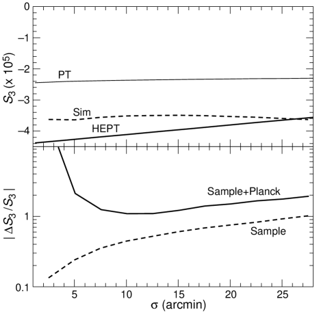
The skewness in our fiducial model is shown for both the perturbation theory and HEPT predictions in Fig. 5.

Since the density bispectrum in both the perturbative and non-linear regime scale as $[P_{\delta}(k)]^{2}$, the amplitude of the underlying density fluctuations roughly scale out of $S_{3}$. However, the pressure bias $b_{\pi}$ does not: $S_{3}\propto b_{\pi}^{-1}$. $S_{3}$ thus provides an observable handle on the bias. This general point applies even if the bias is non-linear although its interpretation will be not be as straightforward (see Fry & Gaztanaga 1993 and Mo, Jing & White 1997 for its application in galaxy biasing).

Figure 6.— One of 500 simulations of the SZ effect in the $\Lambda$CDM model for a $6^{\circ}\times 6^{\circ}$ field-of-view. The range of the map is $-100\mu K,25\mu K$ with an rms of $9\mu K$ and has an approximate angular resolution of $2^{\prime}$. Note the lack of obvious filamentary structures.

Figure 7.— Recovery of the SZ signal with Planck: left to right, model SZ signal, signal $+$ noise from primary anisotropies and foregrounds, and final recovered map from Planck. The signal map is that of Fig. 6 smoothed with a top-hot of radius $20^{\prime}$.

3.6. Numerical Simulations

Since we are interested in the properties of the SZ effect in the weakly-nonlinear regime, cosmological simulations are required to recover the complete statistical properties of the signal and calibrate semi-analytic approaches for its low-order statistics. The simplified SZ model employed in this paper has the virtue that it is easy to simulate as it requires only dark matter and not the gas to model. Its main drawback of course is that results must be taken with a grain of salt due to missing physics.

The realism of the basic approach can be improved by better calibrating the bias model against hydrodynamic simulations. One can envision going beyond the simple redshift dependent bias approach taken here to include scale dependence and stochasticity. Even accounting for these additional complications, simple dark matter simulations can continue to complement full hydrodynamic simulations. Hydrodynamic simulations will always be more limited in dynamic range and sampling volume. Indeed, the current state of the art is limited a handful of realizations across one order of magnitude in physical scale (Refregier et al. 1999; Seljak et al. 2000). A single simulation is then “stacked” on the line-of-sight. Given the range of redshifts at which the SZ effect contributes, the simulation volume is traced many times for each line-of-sight. Moreover, the angular resolution decreases monotonically as one approaches the origin at $z=0$.

The reduction in dynamic range due to the angular projection is a serious but not unfamiliar problem in cosmology. It occurs whenever the kernel for the projection spans cosmological distances. White & Hu (1999) introduced a technique of tiling multiple particle-mesh simulations which telescope along the line of sight to maintain a fixed angular resolution for the analogous problem in weak lensing. This also avoids the problem of over-representing the filamentary structure of the map noted by Refregier et al. (1999).

We refer the reader to White & Hu (1999) for details of the approach and tests of the method. The simulation all have a $256^{3}$ mesh with $256^{2}$ lines of sight for the ray tracing on a $6^{\circ}\times 6^{\circ}$ field. Other relevant parameters are given in Tab. 2: the box size $L_{\rm box}$, the number of particles $N_{\rm part}$, the number of simulations run $N_{\rm sim}$, the number of tiles of the given box size used $N_{\rm tile}$, the maximum redshift to which a given box is used, and the angular resolution of the mesh the maximum and minimum redshift used $\theta_{\rm mesh}$. Note that we cannot shrink the box size along the line-of-sight indefinitely since the fundamental mode of the box must be in the linear regime to provide accurate evolution. This implies that we lose angular resolution near the origin where a fixed physical scale subtends a large angle on the sky. Furthermore at the higher redshift the number of particles must be increased to eliminate shot noise from the initial conditions. Nonetheless, the tiling technique does a good job of maintaining angular resolution at all but the lowest redshifts.

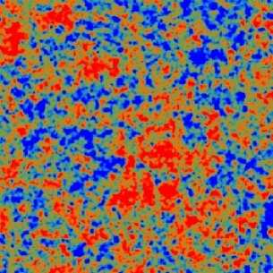
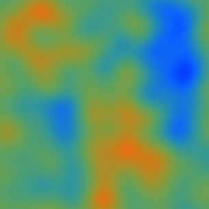
We construct 500 SZ maps from random combinations of the tiles in Tab. 1 for our statistical analysis; one realization is shown in Fig. 6. The average power spectrum is shown in Fig. 4 (top panel) and compared with the linear perturbation theory prediction and the non-linear scaling relation of Peacock & Dodds (1996). We have tested that the deficit of power at the low multipoles is an artifact of the finite field-of-view through monte-carlo realizations of the predicted power spectrum. The roll-off at high multipoles is due to the spatial resolution in the simulations. This also explains the $\sim 10\%$ deficit at intermediate scales which comes from highly non-linear structure close to the origin. Agreement is restored if one eliminates contributions from overdensities $>10$ in the predictions. Since our SZ model is at best valid in the weakly non-linear regime, these contributions should not be included anyway.

Fig. 5 (top panel) shows the results for the skewness in the simulations compared with the second order perturbation theory and HEPT predictions. The agreement here is worse, but is still sufficient for our purposes, given the crudeness of the underlying model for the SZ effect itself.

We can address sample variance questions from the scatter of the results in the individual realizations. Sampling errors for the power spectrum and skewness are shown in the bottom panels of Fig. 4 and 5 respectively. Since these are for individual $6^{\circ}\times 6^{\circ}$ planes, they should be scaled by $\sim 0.03f_{\rm sky}^{-1/2}$ for a given experiment. Sampling errors are one source of noise that we will include in the signal-to-noise calculations in the next section.

Table 2

Details of Numerical Simulations $L_{\rm box}$ $N_{\rm part}$ $N_{\rm sim}$ $N_{\rm tile}$ $z_{\rm max}$ $\theta_{\rm mesh}$ 445 $256^{3}$ 5 2 3.00 $1.4^{\prime}-1.8^{\prime}$ 355 $256^{3}$ 5 2 1.87 $1.4^{\prime}-1.8^{\prime}$ 280 $256^{3}$ 5 2 1.27 $1.4^{\prime}-1.8^{\prime}$ 220 $256^{3}$ 5 2 0.90 $1.4^{\prime}-1.8^{\prime}$ 175 $128^{3}$ 6 2 0.66 $1.4^{\prime}-1.8^{\prime}$ 140 $128^{3}$ 6 2 0.50 $1.4^{\prime}-1.8^{\prime}$ 110 $128^{3}$ 6 2 0.38 $1.4^{\prime}-1.8^{\prime}$ 85 $128^{3}$ 6 2 0.29 $1.4^{\prime}-1.8^{\prime}$ 70 $128^{3}$ 10 9 0.22 $1.4^{\prime}-\infty$

NOTES.—Numerical simulations in our $\Lambda$CDM cosmological model; see text for a description of these quantities.

Figure 8.— Cumulative signal-to-noise in the measurement of the SZ power spectrum with Boomerang, MAP and Planck as a function of maximum $l$. The solid line is the maximum signal-to-noise achievable in a perfect experiment (see text).

4. Estimating the Signal-to-Noise

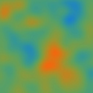
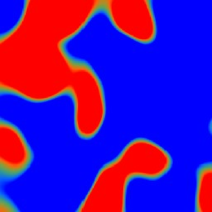
With the SZ signal estimated from the simple bias model of §3 and residual noise calculated from the foreground model and subtraction techniques of §2, we can now estimate the signal-to-noise for the detection of the SZ effect. In Fig. 7, we illustrate the foreground subtraction technique on simulated Planck maps. The signal-to-noise in the maps is of order one for features spanning tens of arcminutes. We shall here show that this level of signal-to-noise is more than sufficient for the purpose of extracting measurements of the low order statistics of the SZ signal.

4.1. Power Spectrum

The signal-to-noise in the power spectrum per multipole $(l,m)$ mode is simply

$$\left({S\over N}\right)_{lm}^{2}={1\over 2}\left({C_{l}^{\rm SZ}\over{C_{l}^{\rm tot}}}\right)^{2}\,.$$ (51)

Here, $C_{l}^{\rm tot}$ is the power spectrum of all contributions in the SZ map,

$$C_{l}^{\rm tot}=C_{l}^{\rm SZ}+N_{l}\,,$$ (52)

where recall that the residual noise $N_{l}$ was defined in equation (10) and includes contributions from detector noise.

Assuming Gaussian statistics for the signal and noise, each mode is independent so that the total signal-to-noise is the quadrature sum

$$\left({S\over N}\right)^{2}={f_{\rm sky}\over 2}\sum_{l}(2l+1)\left({C_{l}^{\rm SZ}\over{C_{l}^{\rm tot}}}\right)^{2}\,.$$ (53)

This quantity gives the variance of the total power measurement in the SZ effect, including sample variance. ${\rm S/N}\gg 1$ means that one has a precise measurement of the power spectrum not simply a highly significant detection. In Fig. 8, for the Boomerang, MAP and Planck experiments as a function of the maximum $l$ mode included in the sum. We also show the ultimate limit of perfect foreground and noise removal where $C_{l}^{\rm tot}=C_{l}^{\rm SZ}$ and $f_{\rm sky}=1$. We will refer to this case here and below as a “perfect experiment”.

With our fiducial choice of the gas bias, Planck should have a highly significant detection of the total signal. One should bear in mind that the bias parameter $b_{\pi}$ is still highly uncertain and that the $S/N$ scales as $b_{\pi}^{2}$. Nevertheless even a relatively large reduction in the average gas temperature or density bias will not make the signal undetectable in principle. In practice, however remember that one is then relying on a precise subtraction of the noise bias in the measurement of $C_{l}^{\rm tot}$, which in turn requires that the power spectrum of the dust and other residual foregrounds lurking at least at the $10\%$ level in rms (1% in power) are determined comparably precisely.

If the fiducial SZ bias is close to correct, the high total single-to-noise in Planck can be used to break the measurement into bands in $l$ and recover the band power with errors

$$\left(\Delta C_{l}^{\rm SZ}\over C_{l}^{\rm SZ}\right)^{-2}={f_{\rm sky}\over 2}\sum_{l_{\rm band}}(2l+1)\left({C_{l}^{\rm SZ}\over C_{l}^{\rm tot}}\right)^{2}\,.$$ (54)

We give an example from monte carlo realizations of the Gaussian noise and sample variance from the simulations in Fig. 4. Note that these are errors for a $6^{\circ}\times 6^{\circ}$ section of the sky and should be scaled by $\sim 0.03f_{\rm sky}^{-1/2}\approx 0.04$ for Planck.

These signal-to-noise estimates assume that both the signal and noise are Gaussian. Of course in reality the SZ signal is non-Gaussian. In general, gravitational collapse correlates the amount of power in density fluctuations across all scales in the non-linear regime. However since the SZ effect probes many independent density fluctuations along the line-of-sight, the central limit theorem ensures that the SZ signal is far more Gaussian than the density field. We can test how much this affects the signal-to-noise with our simulations. Shown in Fig. 4 is the sampling errors on the band powers from the simulations themselves as compared with those from Gaussian realizations of the same power spectrum. The excess variance over the Gaussian limit is small on the relevant scales given detector noise limitations from Planck.

Figure 9.— Cumulative signal-to-noise in the measurement of the third moment, $\Theta^{3}$, with top hat smoothing in multipole space (i.e. truncation above $l_{\rm max}$). The HEPT approximation to the bispectrum is assumed here. MAP and Boomerang (not shown) have signal-to-noise values less than $0.1$ everywhere.

4.2. Skewness

The overall signal-to-noise for the measurement of the third moment of SZ effect is

$$\left({S\over N}\right)^{2}={f_{\rm sky}}{\left<\Theta^{3}(\hat{\bf n};\sigma)\right>^{2}\over{\rm Var}}$$ (55)

where the variance is given by

$${\rm Var} = {1\over(4\pi)^{2}}\sum_{l_{1}l_{2}l_{3}}{(2l_{1}+1)(2l_{2}+1)(2l_{3}+1)\over 4\pi}\left(\begin{array}[]{ccc}l_{1}&l_{2}&l_{3}\\ 0&0&0\end{array}\right)^{2}$$ (59)

$$\times W_{l_{1}}^{2}(\sigma)W_{l_{2}}^{2}(\sigma)W_{l_{3}}^{2}(\sigma)6C_{l_{1}}^{\rm tot}C_{l_{2}}^{\rm tot}C_{l_{3}}^{\rm tot}\,.$$

In Fig. 9, we show the signal-to-noise for a measurement of the third moment as calculated under the HEPT. We compare the signal-to-noise in Planck with the ideal case of perfect removal of foregrounds and detector noise, and full sky coverage. We use here a tophat window in multipole space out to $l_{\rm max}$ to conform with other signal-to-noise considerations. Cosmic variance and Planck detector noise reduces the signal-to-noise values both at the low and high end for $l_{\rm max}$ values respectively. For Planck, the $l$ values in the range of few hundred to $\sim$ 1000 provides the maximal signal-to-noise for a measurement of the skewness. This corresponds to smoothing scales $\sigma\sim$ 10’-30’ for tophat windows in angular space (c.f. Fig. 5). For MAP and Boomerang, the signal-to-noise values are $\lesssim$ 0.1, suggesting that a detection of SZ skewness is not likely to be possible in these two experiments.

Again equation (59) assumes Gaussian statistics for the variance and ignores the sample variance of the third moment itself. We test this approximation in Fig. 5 and find that it is reasonable given the level of residual noise for Planck. In constructing an estimator for $S_{3}$, it is important to remove the noise bias since noise variance will always reduce the skewness in the map. We do this by multiplying the estimator by $(\left<\Theta_{\rm tot}^{2}\right>/\left<\Theta_{\rm SZ}^{2}\right>)^{2}$.

Finally, note that in the noise-dominated regime the signal-to-noise in $S_{3}$ scales strongly with the gas bias $S/N\propto b_{\pi}^{3}$, so that the detectability of this effect depends strongly on currently uncertain assumptions.

Figure 10.— Cumulative signal-to-noise for the detection of SZ bispectrum as a function of $l_{3}$ multipole. The solid line is the maximum signal-to-noise achievable in a perfect experiment.

4.3. Bispectrum

The full bispectrum of the SZ effect contains all of the information about its three-point correlations induced by the growth of structure beyond the linear approximation. The skewness is simply one, easily measured, aspect of the bispectrum. The full signal-to-noise ratio of the bispectrum is

$$\left({S\over N}\right)^{2}=f_{\rm sky}\sum_{l_{1},l_{2},l_{3}}{B_{l_{1}l_{2}l_{3}}^{2}\over 6C_{l_{1}}^{\rm tot}C_{l_{2}}^{\rm tot}C_{l_{3}}^{\rm tot}}\,,$$ (60)

where $C_{l}^{\rm tot}$ follows Eq. (52). We plot the bispectrum cumulative signal-to-noise as a function of signal $l_{3}$, summed over $l_{1}$ and $l_{2}$. We refer the reader to Cooray & Hu (1999) for a detailed discussion on the bispectrum, its variance and the calculation of signal-to-noise ratio.

In Fig. 10, we show the expected cumulative signal-to-noise for the SZ bispectrum in Boomerang, MAP and Planck data and a perfect experiment. The signal-to-noise is calculated under the HEPT approximation for the underlying density field. As shown, MAP and Boomerang allow reasonable limits to be placed on any non-Gaussian signal in the SZ effect while Planck allows a strong possibility for a detection.

Again the same caveats as to the sensitivity of the $S/N$ estimate to the underlying assumptions that applied for the skewness also apply here. Moreover, measuring all the configurations of the bispectrum will be a formidable computational challenge as will control over systematic effects in the experiments.

4.4. Lensing Correlation

The SZ effect and weak gravitational lensing of the CMB both trace large-scale structure in the underlying density field. By measuring the correlation, one can directly test the manner in which gas pressure fluctuations trace the dark matter density fluctuations. The correlation vanishes in the two-point functions since the lensing does not affect an isotropic CMB due to conservation of surface brightness.

The correlation manifests itself as a non-vanishing bispectrum in the CMB at RJ frequencies (Goldberg & Spergel 1999; Cooray & Hu 1999). Again the cosmic variance from the primary anisotropies presents an obstacle for detection of the effect above the several arcminute scale ($l\sim 2000$). With the multifrequency cleaning of the SZ map presented here one can enhance the detectability of the effect.

Consider the bispectrum composed of one $a_{lm}$ from the cleaned SZ map and the other two from the CMB maps. Call this the SZ-CMB-CMB bispectrum. The noise variance of this term will be reduced by a factor of $C_{l}^{\rm tot}/C_{l}^{\rm CMB}$ compared with the CMB-CMB-CMB bispectrum. As one can see from Fig. 1 this can be up to a factor of $10^{3}$ in the variance. Details for the calculation of the CMB-CMB-CMB bispectrum are given in Cooray & Hu (1999). Here we have updated the normalization for SZ effect, taken $f_{{\rm sky}}=0.65$ for Planck’s useful sky coverage, and compared the $S/N$ of the two bispectra. As shown, the measurement using foreground cleaned Planck SZ and CMB maps has a substantially higher signal-to-noise than that from using the Planck CMB map alone for multipoles $l\sim 10^{2}-10^{3}$.

Beyond the improvement in signal-to-noise, however, there is an important advantage in constructing the SZ-lensing bispectrum using SZ and CMB maps. A mere measurement of the bispectrum in CMB data can lead to simultaneous detection of non-Gaussianities through processes other than just SZ-lensing cross-correlation. As discussed in Goldberg & Spergel (1999) and extended in Cooray & Hu (1999), gravitational lensing also correlates with other late time secondary anisotropy contributors such as integrated Sachs-Wolfe (ISW; Sachs & Wolfe 1967) effect and the reionized Doppler effect. In addition to lensing correlations, non-Gaussianities can also be generated through reionization and non-linear growth of perturbations (Spergel & Goldberg 1999; Goldberg & Spergel 1999; Cooray & Hu 1999). Bispectrum measurements at a signle frequency can result in a confusion as to the relative contribution from each of these scenarios. In Cooray & Hu (1999), we suggested the possibility of using differences in individual bispectra as a function of multipoles, however, such a separation can be problematic given that these differences are subtle (e.g., Fig 6 of Cooray & Hu 1999).

The construction of the SZ-lensing bispectrum using SZ and CMB maps has the advantage that one eliminates all possibilities, other than SZ, that result in a bispectrum. For effects related to SZ, the cross-correlation of lensing and SZ should produce the dominant signal; as shown in Cooray & Hu (1999), bispectra signal through SZ and reionization effects, such as Ostriker-Vishniac (OV; Ostriker & Vishniac 1986), are considerably smaller.

Conversely, multifrequency cleaning also eliminates the SZ contribution from the CMB maps and hence a main contaminant of the CMB-CMB-CMB bispectrum. This assists in the detection of smaller signals such as the ISW-lensing correlation, Doppler-lensing correlation or the non-Gaussianity of the initial conditions. Such an approach is highly desirable and Planck will allow such detailed studies to be carried out.

A potential caveat is that as noted above, the full bispectrum in an all-sky satellite experiment will be difficult to measure. Zaldarriaga & Seljak (1999) have developed a reduced set of three-point statistics optimized for lensing studies, based on a two point reconstruction of the lensing-convergence maps from temperature gradient information. They show that most of the information is retained in these statistics. Multifrequency cleaning improves the signal-to-noise for these statistics by exactly the same factor as for the full bispectrum.

Figure 11.— Cumulative signal-to-noise in the measurement of the SZ-weak gravitational lensing cross-correlation through the bispectrum measurement in CMB data. Compared are the expected signal-to-noise with (SZ-CMB-CMB) and without (CMB-CMB-CMB) multifrequency isolation of the SZ effect for Planck and a perfect/cosmic variance limited experiment. Multifrequency isolation provides additional signal-to-noise and the opportunity to uniquely identify the bispectrum contribution with the SZ effect.

5. Discussion

We have studied the prospects for extracting the statistical properties of the Sunyaev-Zel’dovich (SZ) effect associated with hot gas in large-scale structure using upcoming multifrequency CMB experiments. This gas currently remains undetected but may comprise a substantial fraction of the present day baryons. The SZ effect has a distinct spectral dependence with a null at a frequency of $\sim$ 217 GHz compared with true temperature anisotropies. This frequency dependence is what allows for effective separation of the SZ contribution with multifrequency CMB measurements.

As examples, we have employed the frequency and noise specifications of the Boomerang, MAP, Planck experiments. The MAP satellite only covers frequencies at RJ part of the frequency spectrum. Consequently, only Boomerang and Planck can take full advantage of multifrequency separation of the SZ and primary anisotropies. We have evaluated the detection threshold for SZ power spectrum measurements (see Fig. 3). Boomerang and MAP should provide limits on the degree scale fluctuations at the several $\mu$K level in rms; Planck should be able to detect sub $\mu$K signals.

The expected level of the SZ signal in the fiducial $\Lambda$CDM model is still somewhat uncertain. We have employed a simple bias model for the pressure fluctuations, roughly normalized to recent hydrodynamic simulations (Refregier et al. 1999; Seljak et al. 2000), and calculated the resulting signal using analytic scaling relations and particle-mesh dark matter simulations. As hydrodynamic simulations improve, these techniques can be extended with more sophisticated modeling of the bias. They complement hydrodynamic simulations by extending the dynamic range and simulated volume, the latter being important for questions of sample variance.

Assuming this simplified model of the SZ signal, Planck should have signal-to-noise per multipole of order unity for $l<1000$. Although the recovered maps are then somewhat noisy, they are sufficient for precise determinations of low order statistics such as the SZ power spectrum, bispectrum and skewness (see Figs. 4-10). The skewness in principle can be used to separate the pressure bias from the underlying amplitude of the density fluctuations. The full bispectrum contains significantly more information but will be difficult to extract in its entirety. Current methods for measuring the bispectrum, tested with the COBE data, have concentrated at measuring specific modes such as $l_{1}=l_{2}=l_{3}=l$ (Ferreira et al. 1998). More work will clearly be required, especially in understanding the systematic errors at a sufficient level, but the wealth of information potentially present in the bispectrum should motivate efforts.

Note however that the non-Gaussianity in the SZ signal is not very strong due to the fact that it is constructed from many independent pressure fluctuations along the line of sight. As a consequence, we expect that signal-to-noise ratios can be estimated by Gaussian approximations, but that techniques that try to improve the SZ-primary separation based on non-Gaussianity (Hobson et al 1998; Aghanim & Forni 1999) may not be particularly effective for this signal.

We caution the reader that our oversimplification of the SZ signal can cause problems for a naive interpretation of future detections. For example, Seljak et al. (2000) find that the SZ power spectrum in their simulations is dominated by shot noise from the rare hot clusters not included in our modeling. Fortunately since these contributions are highly non-Gaussian, they can can readily be identified and removed. At the very least, $X$-ray bright clusters can be externally identified and removed; this has been shown to substantially reduce the shot noise contribution (Komatsu & Kitayama 1999). The effect we are modeling should be understood as the signal in fields without such clusters.

Another means of separating the SZ signal from large-scale structure from that of massive clusters is to cross correlate it with other tracers of large-scale structure that are less sensitive to highly overdense regions. An added benefit is that such a cross-correlation will also empirically measure the extent to which pressure fluctuations follow mass fluctuations. The CMB anisotropies themselves carry one such tracer in the form of the convergence from weak lensing. It manifests itself as a three-point correlation or bispectrum (Goldberg & Spergel 1999) but without frequency information it is severely sample-variance limited due to confusion noise from primary anisotropies. Measuring the SZ-lensing correlation using the cleaned SZ maps improves the signal-to-noise for the detection by over an order of magnitude at degree scales. Furthermore, the techniques introduced by Zaldarriaga & Seljak (1999) provide a concrete algorithm for extracting most of the three-point signal without recourse to measuring all the configurations of the bispectrum. Conversely, SZ removal from the CMB maps themselves can assist in the detection of other smaller bispectrum signals by eliminating one source of confusion noise.

The cross-correlation coefficient between the SZ effect and CMB weak lensing is relatively modest ($\sim$ 0.5, see Seljak et al. 2000). This is due to the fact that the SZ effect is a tracer of the nearby universe while CMB lensing is maximally sensitive to structure at $z\sim 3$. A higher correlation is expected if SZ is cross-correlated with an external probe of low redshift structure. Peiris & Spergel (2000) suggested the cross-correlation of MAP CMB data and Sloan galaxy data. An improved approach would be to use the Planck derived SZ map rather than a CMB map. Using a SZ map reduces noise from the primary anisotropies and guarantees that any detection is due to correlations with the SZ effect. Extending the calculations in Peiris & Spergel (2000) with the Planck generated SZ map, we find signal-to-noise ratios which are on average greater by a factor of $\sim$ 10 when compared to signal-to-noise values using MAP CMB map. In fact with redshifts for galaxies, Planck SZ map can be cross-correlated in redshifts bins to study the redshift evolution of the gas. Other promising possibilities include cross correlation with soft X-ray background measurements, as well as ultraviolet and soft X-ray absorption line studies.

All these considerations imply a bright future for SZ studies of the hot gas associated with large-scale structure with wide-field multifrequency CMB observations. Its detailed properties should be revealed in its non-Gaussianity and correlation with other tracers of large-scale structure.

References

- (1) Aghanim, N., Desert, F.X., Puget, J.L, & Gispert, R. 1996, A&A, 311 1
- (2) Aghanim, N., Forni, O. 1999, A&A, 347 409
- (3) Bouchet, F., Gispert, R., 1999, NewA, 4 443
- (4) Briel, U. G., Henry, J. P., 1995, A&A, 302, L9
- (5) Bouchet, F. R. et al. 1995, Space Sci Rev., 84, 37
- (6) Bunn, E. F., White, M. 1997, ApJ, 480, 6
- (7) Carlstrom, J. E., Joy, M., Grego, L. 1996, ApJ, 456, L75
- (8) Cen, R., Kang, H., Ostriker, J. P., Ryu, D. 1995, ApJ, 451, 436
- (9) Cen, R., Ostriker, J. P. 1999, ApJ, 514, 1
- (10) Cooray, A. R., Hu, W. 1999, ApJ in press, astro-ph/9910397
- (11) da Silva, A. C., Barbosa, D., Liddle, A. R., Thomas, P. A. 1999, MNRAS, submitted, astro-ph/9907224
- (12) Ferreira, P.G., Magueijo, J., Gorksi, K.M. 1998, ApJ, 503, 1
- (13) Fry, J.N., Gaztanaga, E. 1993, ApJ, 413 447
- (14) Fukugita, M., Hogan, C. J., Peebles, P. J. E. 1998, ApJ, 503, 518
- (15) Goldberg, D. M., Spergel, D. N. 1999, PRD, 59, 103002
- (16) Haehnelt M. G., Tegmark, M. 1996, MNRAS, 279, 545
- (17) Hobson, M. P., Jones, A. W., Lasenby, A. N., Bouchet, F. R. 1998, MNRAS, 299, 895
- (18) Hu, W. 2000a, ApJ, 529, 12
- (19) Hu, W. 2000b, PRD submitted, astro-ph/0001303
- (20) Hui, L. 1999, ApJ, 519, L9
- (21) Jones, M. Saunders, R., Alexander, P., et al. 1993, Nat, 365, 320
- (22) Jungman, G., Kamionkowski, M., Kosowsky, A., Spergel, D.N., 1996, Phys. Rev. D, 54, 1332
- (23) Komatsu, E. Kitayama, T., 1999, ApJ, 526, L1
- (24) Kull, A., Böhringer, H. 1999, A&A, 341, 23
- (25) Limber, D. 1954, ApJ, 119, 655
- (26) Mo, H.J., Jing, Y.P., White, S.D.M. 1997, MNRAS, 284, 189
- (27) Ostriker, J.P., Vishniac, E.T. 1986, Nature, 322, 804
- (28) Peacock, J.A., Dodds, S.J. 1996, MNRAS, 280, L19
- (29) Pen, U.-L. 1999, ApJ, 510, 1
- (30) Persi, F. M., Spergel, D. N., Cen, R., Ostriker, J. P. 1995, ApJ, 442, 1
- (31) Peiris, H. V., Spergel, D. N. 2000, ApJ submitted, astro-ph/001393
- (32) Pointecouteau, E., Giard, M., Barret, D. 1998, A&A, 336, 44
- (33) Refregier, A., Komatsu, E., Spergel, D. N., Pen, U.-L. 1999, PRD submitted, astro-ph/9912180
- (34) Sachs, R. K., Wolfe, A. M., 1967, ApJ, 147, 73
- (35) Scharf, C., Donahue, M., Voit, G. M., Rosati, P., Postman, M. 2000, ApJ, 528, L73
- (36) Scoccimarro, R., Frieman, J. A. 1999, ApJ, 520, 35
- (37) Seljak, U, Burwell, J., Pen, U.-L. 2000, PRD submitted, astro-ph/001120
- (38) Seljak, U., Zaldarriaga, M. 1996, ApJ, 469, 437
- (39) Spergel, D. N., Goldberg, D. M. 1999, PRD, 59, 103001
- (40) Sunyaev, R.A., Zel’dovich, Ya. B. 1980, MNRAS, 190, 413
- (41) Tegmark, M., Eisenstein, D.J., Hu, W., de Oliveira-Costa, A. ApJ, 1999, in press, astro-ph/9905257
- (42) White, M., Hu, W., 1999, ApJ in press, astro-ph/9909165
- (43) Zaldarriaga, M., Seljak, U. 1999, Phys. Rev. D. 59, 123507