Euler–Poincaré reduction and the Kelvin–Noether theorem for discrete mechanical systems with advected parameters and additional dynamics
Abstract
The Euler–Poincaré equations, firstly introduced by Henri Poincaré in 1901, arise from the application of Lagrangian mechanics to systems on Lie groups that exhibit symmetries, particularly in the contexts of classical mechanics and fluid dynamics. These equations have been extended to various settings, such as semidirect products, advected parameters, and field theory, and have been widely applied to mechanics and physics. In this paper, we introduce the discrete Euler–Poincaré reduction for discrete Lagrangian systems on Lie groups with advected parameters and additional dynamics, utilizing group difference maps. Specifically, the group difference map is defined using either the Cayley transform or the matrix exponential. The continuous and discrete Kelvin–Noether theorems are extended accordingly, that account for Kelvin–Noether quantities of the corresponding continuous and discrete Euler–Poincaré equations. As an application, we show both continuous and discrete Euler–Poincaré formulations about the dynamics of underwater vehicles, followed by numerical simulations. Numerical results illustrate the scheme’s ability to preserve geometric properties over extended time intervals, highlighting its potential for practical applications in the control and navigation of underwater vehicles, as well as in other domains.
1 Introduction
Many physical systems exhibit symmetries, such as invariance under translation, rotation, or particle relabeling. Symmetries can be used to simplify the dynamics by reducing the degrees of freedom or the order of an invariant system (e.g., [35, 43]). In Lagrangian mechanics, the symmetries of a Lagrangian, specifically its invariance under Lie group actions, enable the reduction of the corresponding Euler–Lagrange equations (i.e., the equations of motion), for example, through the use of invariantized coordinates. More generally, this can be extended to symmetries of functionals, also known as least actions. One of the reduction methods, called Euler–Poincaré reduction, leads to the Euler–Poincaré equations, is a particular case of Lagrangian reduction when the configuration space is a Lie group and the Lagrangian is -invariant [37, 38]. It has been widely applied in rigid body dynamics [30], fluid mechanics [2], magnetohydrodynamics [22], plasma physics [24, 49], thermodynamical simple systems [11], etc. The Euler–Poincaré equations can also be expressed in terms of the Lie–Poisson equations via the reduced Legendre transformation.
Reduction theory in discrete mechanics is also often approached from a variational perspective, as demonstrated in [40, 50]. These variational integrators are known to play a crucial role in the numerical integration of mechanical systems and geometric mechanics [27, 51]. Some pioneering work on discretizations of reduction theory includes [4, 17]. In particular, the discrete analogue of the Euler–Poincaré reduction has been studied in [16, 34, 45]. Implementing numerical iterations of the discrete Euler–Poincaré equations in the (linear) Lie algebra rather than directly using the Lie group-valued Euler–Lagrange equations involves a discretization strategy that focuses on the algebraic structure, simplifying the computations by working with the Lie algebra rather than the more complex Lie group.
The Euler–Poincaré reduction has been investigated in various contexts (e.g., [7, 36]). Recently, in [20], the authors proposed (continuous) Euler–Poincaré reduction with advected parameters and additional dynamics, which was applied to study the dynamics of the wave mean flow interaction. In this paper, we develop the discrete analogue of the Euler–Poincaré reduction incorporated advected parameters and additional dynamics and then propose the corresponding discrete Euler–Poincaré equations with additional dynamics.
The contributions of this study are summarized below.
-
(1)
The discrete Euler–Poincaré reduction for Lagrangian mechanics with advected parameters and additional dynamics is formulated.
-
(2)
The Kelvin–Noether theorem and its discrete analogue are generalized to systems with additional dynamics and advected parameters.
-
(3)
The discrete Euler–Poincaré reduction is applied to the dynamics of underwater vehicles by deriving both the continuous and discrete Euler–Poincaré equations. The behavior of the total energy and Kelvin–Noether quantity is also presented to demonstrate the efficiency of the scheme.
This paper is structured as follows. In Section 2, we recall the Euler–Poincaré reduction for systems with and without advected parameters and additional dynamics and extend the Kelvin–Noether theorem to incorporate advected parameters and additional dynamics simultaneously. In Section 3, the discrete counterpart of the theories introduced in Section 2 is developed by using the discrete variational calculus. In Section 4, the discrete Euler–Poincaré reduction with advected parameters and additional dynamics is applied to the dynamics of underwater vehicles. We derive the numerical schemes and the discrete Kelvin–Noether quantities in cases that the group difference map is chosen as either the Cayley transform or the matrix exponential. In Section 5, we present numerical results for the dynamics of underwater vehicles, focusing on the behavior of the total energy and the Kelvin–Noether quantity. Finally, we conclude and discuss directions of future research in Section 6.
2 The continuous Euler–Poincaré reduction
Consider a mechanical system with a configuration space , an -dimensional smooth manifold, and let be a Lie group acting smoothly on . In the current study, left group actions will be considered unless otherwise specified. The action of a group element on a point is denoted as , while its tangent lift to is denoted by . Consider a smooth curve for and its tangent vector . In the following, the time variable is omitted for brevity. A Lagrangian defined in the tangent bundle , , is -invariant if
| (1) |
If and choosing left action of , the (left) reduced Lagrangian defined on the Lie algebra can be derived as
| (2) |
where and is the identity element. Associated with it, the ‘basic’ Euler–Poincaré equations hold (e.g., [3, 37, 38, 48])
| (3) |
where the adjoint operator is defined by using the Lie bracket as
| (4) | ||||
and the coadjoint operator for left action is defined as the pairing between and its dual ,
| (5) |
Importance of the Euler–Poincaré equations (3) (e.g., its relation to nonholonomic constraints and its Hamiltonian character) was first recognized by Hamel [18, 19] and Chetayev [9].
Analogous to the equivalence of the Euler–Lagrange equations for a regular Lagrangian defined om the tangent bundle and Hamilton’s equations on the cotangent bundle through the Legendre transformation, the Euler–Poincaré equations (3) are similarly equivalent to the Lie–Poisson equations
| (6) |
where the Legendre transformation between and defines
| (7) |
and is the reduced Hamiltonian defined on ,
| (8) |
It follows immediately that
| (9) |
2.1 The Euler–Poincaré equations with advected parameters
Holm et al. studied mechanical systems with advected parameters in a dual vector space within the Lagrangian semidirect product theory [21]. However, it was also pointed out therein that the Euler–Poincaré equations with advected parameters are not the Euler–Poincaré equations derived from the semidirect product Lie algebra. Advected parameters often appear, for instance, when a potential function in a Lie group is involved, and they bear dynamical significance in the reduction context. For instance, in the case of the heavy top, the parameter corresponds to the unit vector aligned with gravity. In the context of compressible flows, it represents the fluid density in the reference configuration. The following theorem for the Euler–Poincaré equations with advected parameters was shown in [21].
Theorem 1.
Let be a Lie group that acts on a dual vector space from the left. Assume that the Lagrangian is left -invariant. When , the corresponding function , defined by , is left -invariant, where denotes the isotropy group of . The -invariance of allows one to define by
| (10) |
For a curve on , let and define a curve for the advected parameters . Their variations satisfy
| (11) |
where and is the Lie derivative with respect to . Therefore, Hamilton’s principle for the action leads to the (left-left444In the current study, left group actions of on are considered and the Lagrangians are assumed to be left invariant too.) Euler–Poincaré equations on :
| (12) |
and the curve is the unique solution of the linear differential equation
| (13) |
with initial condition , and the diamond operator is the bilinear operator defined by
| (14) |
for all , , and .
2.2 The Euler–Poincaré equations with advected parameters and additional dynamics
In this section, we recall the Euler–Poincaré equations with advected parameters and additional dynamics introduced in [20]. Consider as the configuration space and the curves in for with tangent vectors and . A Lagrangian defined in with advected parameters can be defined as
| (15) | ||||
Invariance of the Lagrangian under the left action of reads
| (16) |
Assuming that , the reduced Lagrangian can be defined as the function ,
| (17) |
where , , , and . Defining and , the variations of , and can be calculated as follows:
| (18) |
where we have used the definitions and . Note that is defined by the infinitesimal generator at , , or the Lie algebra action of the manifold , as [8]
| (19) |
The variations and are arbitrary and vanish at fixed endpoints of the time interval . From the above variations and Hamilton’s principle, the Euler–Poincaré equations with the advected parameter in and the additional dynamics in can be derived as follows:
| (20) | ||||
and the curve is again the unique solution of
| (21) |
The complementary relation of reads
| (22) |
Here, the operator is defined by the pairing
| (23) |
and representation of the diamond operator in follows from that used in [20], which is (local) decomposition of the operator (corresponding to the Lie group acting on the manifold ) defined as
| (24) |
2.3 The continuous Kelvin–Noether theorem
The Kelvin–Noether theorem combines ideas from Kelvin’s circulation theorem and Noether’s theorem. It relates the conservation of circulation in a fluid to the underlying symmetries of the fluid’s dynamics, particularly those arising from its Lagrangian formulation and the associated Lie-group symmetries [16, 21].
The Noether’s theorem states that every finite-dimensional variational Lie group symmetry gives rise to a conservation law of the Euler–Lagrange equations (e.g., [41, 43]). Discrete and semi-discrete extensions of this theorem have also been proposed (e.g., [39, 46, 47]). In particular, for Euler–Poincaré equations, this extends the Kelvin’s circulation theorem for continuum mechanics and is called the Kelvin–Noether theorem (e.g., [10, 16, 21]). Next we introduce the Kelvin–Noether theorem for Euler–Poincaré equations with advected parameters and additional dynamics. Note that in the current study, the Lie group is assumed to be finite-dimensional, and hence .
Theorem 2.
Let be a group acting on a manifold and a vector space both from the left. Consider an equivalent map , that is,
| (25) |
for any , and . The adjoint action is defined by the tangent map of the left and right multiplications and (for ) at the identity as
| (26) |
Furthermore, consider a path satisfying the Euler–Poincaré equations (20) and the advected parameter dynamics (21). For with and , define the (left-left) Kelvin–Noether quantity by
| (27) |
which satisfies that
| (28) |
Proof.
The proof is similar to that in [21, 23], with an extension to account for the additional dynamics. Recall that , , and are time-dependent. For any , we have
| (29) | ||||
Taking the derivative of the Kelvin–Noether quantity (27) and taking the Euler–Poincaré equations (20) into consideration, we obtain
| (30) | ||||
which completes the proof. Note that we have used the formula for differentiating the coadjoint action [23, 35], namely,
| (31) | ||||
∎
3 The discrete Euler–Poincaré equations with advected parameters and additional dynamics
In this section, we show the discrete Euler–Poincaré equations with advected parameters and additional dynamics. Before showing its derivation by the discrete variational principle, let us recall the group difference map and some of its properties, following [5, 6, 16].
Definition 3.
(Group difference map.) A local diffeomorphism that maps a neighborhood of to a neighborhood of identity , such that and for all , is called a group difference map.
Definition 4.
(Right-trivialized tangent.) The right-trivialized tangent map of a group difference map is defined by
| (32) |
This was defined in [26] (Definition 2.19 therein), which describes the differential of as a combination of a map and the right transport of the tangent vector from to . Moreover, the right-trivialized tangent satisfies the following relation
| (33) |
Definition 5.
(Inverse right-trivialized tangent.) The inverse right-trivialized tangent of a group difference map is defined by
| (34) |
This definition describes that the differential of can be decomposed into the right transport of the tangent vector from to and the map . The inverse right-trivialized tangent satisfies
| (35) |
Now we consider reduced discrete Lagrangians and derive the discrete Euler–Poincaré equations with advected parameters and addition dynamics, which extends the results of [16]. Let be the discretized time for and be a fixed time step. Consider discrete series on the Lie group and on the additional configuration manifold . (Left) -invariance of the discrete Lagrangian , namely
| (36) |
defines the (left) reduced discrete Lagrangian by taking ,
| (37) |
denoted by , with
| (38) |
and the advected parameter
| (39) |
Note that the defined in (38), which can be equivalently written as
| (40) |
is the forward Euler formula on Lie groups for introduced in the continuous setting (e.g., [5, 6]).
The corresponding discrete functional reads
| (41) |
The discrete variational principle is expressed as for arbitrary variations and , and subject to fixed endpoint conditions and . This leads to the following discrete Euler–Poincaré equations through discrete variational calculus.
Theorem 6.
Let act from the left on the dual vector space and let the discrete Lagrangian be left -invariant. Let be the reduced Lagrangian defined by (37). Suppose is a discrete series satisfies under variations and with and . Then we obtain the (left-left) discrete Euler–Poincaré equations with advected parameters and additional dynamics:
| (42) | ||||
together with the complementary relation
| (43) |
and is given by the series
| (44) |
Analogous to the continuous case (24), the diamond operator corresponding to the Lie group G acting on the manifold in the discrete setting is again defined pointwisely in as
| (45) |
The diamond operator in is defined in a similar way but at another point . Furthermore, the action is defined by
| (46) |
for or .
Proof.
First, the variation of is obtained by using (35) as [6, 16]
| (47) |
Introducing the variations and , the variations of and can be calculated using the relations (38) and (39) directly, and we obtain
| (48) |
Using the fixed endpoint condition, the discrete variational principle then gives
| (49) | ||||
which yields the discrete Euler–Poincaré equations (42). ∎
The discrete Kelvin–Noether theorem. The following theorem describes a discrete analogue of the continuous Kelvin–Noether Theorem 2. Again, we assume that the Lie group is finite-dimensional, and hence .
Theorem 7.
Let be a Lie group that acts on a manifold from the left and suppose is an equivalent map, namely
| (50) |
for any , and . Suppose the discrete series satisfies the (left-left) discrete Euler–Poincaré equations (42) and the discrete advected parameter dynamics (44). Fix and define . We then define the discrete (left-left) Kelvin–Noether quantity by
| (51) |
where is a given group difference map. As a consequence, the discrete Kelvin–Noether quantity satisfies
| (52) |
4 Application to the dynamics of underwater vehicles
In this section, the proposed Euler–Poincaré reduction for systems with advected parameters and additional dynamics is applied to study the behavior of underwater (or submersible) vehicles. Underwater vehicle dynamics has been studied from both practical and theoretical perspectives (e.g., [12, 15, 44]), particularly using geometric mechanics (e.g., [31, 42]). We consider underwater vehicles with added mass, also known as hydrodynamic or virtual mass, which affects the inertia matrix of the vehicles. Additionally, we assume that the center of gravity of the underwater vehicle does not coincide with its center of buoyancy. This is a practical design feature, as underwater vehicles are typically constructed with the center of gravity positioned below the center of buoyancy (i.e., bottom-heavy) to ensure stability [31].
In this case, the Lie group is the 3-dimensional special orthogonal group
| (53) |
and its associated Lie algebra is
| (54) |
where is the identity matrix. In the dynamics of underwater vehicles, the rotation matrix represents the attitude of the body and also serves as a map from a reference configuration to the body configuration. The differential of with respect to reads
| (55) |
This implies that the body angular velocity matrix , which is related to the body angular velocity vector through the Lie algebra isomorphism
| (56) | ||||
In this paper, we follow [16] and define the pairing between and its dual as such that for any , where denotes the trace of matrices.
Continuous case. In the dynamics of underwater vehicles, the kinetic energy is expressed as
| (57) |
where the first and second terms come from linear motion of vehicles and the hydrodynamic added mass, and the third term represents the rotational kinetic energy. Inner product of vectors in Euclidean spaces is denoted by . The potential energy corresponding to the gravitational and buoyancy restoring forces is given by
| (58) |
where the term represents the gravitational potential energy and the remaining term represent the buoyant potential energy. Here, we denote the vehicle’s mass by , its volume by , the hydrodynamic added mass matrix by assumed to be symmetric for simplicity, and the fluid’s density by . The constant vector denotes the position of the center of buoyancy as seen from the (center of the gravity of) vehicle, and the gravitational constant is . The vector is the unit vector along the vertical axis of the space-fixed frame. Furthermore, the modified inertia tensor is related to the inertia tensor in the space-fixed frame via
| (59) |
Note that while the inertia tensor is a symmetric, positive-definite matrix, the modified inertia tensor is not necessary positive-definite.
The total energy is , while the Lagrangian is defined by
| (60) | ||||
Here, , and . Left-invariance of the Lagrangian can be immediately checked that
| (61) |
and the reduced Lagrangian is defined by taking in the action as
| (62) | ||||
where , and the advected parameter is .
Defining and , we can derive the variations of , analogous to (18) as follows:
| (63) |
Define the reduced functional as
| (64) |
and the Euler–Poincaré equations (20) for underwater vehicle dynamics can directly be calculated, which read
| (65) | ||||
and satisfies with initial values , where . The complementary relation between reads . The following lemma is applied here (e.g., [16]).
Lemma 8.
For any ,
-
•
;
-
•
the diamond operator is given by .
Discrete case. We discretize the translational velocity by the forward difference
| (66) |
and the relation by the forward Euler formula
| (67) |
and hence . The discrete kinetic energy is given by
| (68) |
while the discrete potential energy is given by
| (69) |
This gives the discrete total energy , and the discrete Lagrangian
| (70) |
Invariance of the discrete Lagrangian defines a reduced discrete Lagrangian , denoted by , as follows
| (71) | ||||
where
| (72) |
Substituting the Lagrangian (71) to (42) amounts to the discrete Euler–Poincaré equations for the underwater vehicle dynamics as follows:
| (73) | ||||
together with , and the advected parameter satisfies , where .
Remark 9.
Since the additional dynamics is in the linear space , we may introduce the quantity , and the equations above can be rewritten as
| (74) | ||||
Discrete Kelvin–Noether quantities. Let act on through the adjoint representation
| (75) |
for where . Let () be the equivariant map . Define
| (76) | ||||
the discrete Kelvin–Noether Theorem 7 yields
Note that , which becomes by choosing as the initial value . Consequently, , namely,
| (77) | ||||
is a constant of motion. Thus, equations (73) preserve the -component of the vector, which is the inverse of the following matrix by using the Lie algebra isomorphism (56):
| (78) |
Next, let us consider some well-known group difference maps .
Cayley transform as the group difference map. Let the map be the Cayley transform:
| (79) |
and the dual of its right-trivialized tangent is given by [16]
| (80) |
Then the discrete Euler–Poincaré equations (74) become
| (81) | ||||
To facilitate simulation, we will vectorize the first equation of (81) using the following lemma.
Lemma 10.
For any , a real symmetric matrix and matrix we have the identities
| (82) |
| (83) |
| (84) |
| (85) |
Proof.
∎
Based on the lemma above, recalling and denoting , the first equation of (81) can be vectorized as follows
| (88) | ||||
which is implicit in . Therefore, we use the Gauss–Newton method for solving ,
| (89) |
Its differential with respect to is
| (90) |
Matrix exponential as the group difference map. The matrix exponential can also be regarded as the group difference map . On the Lie group , the matrix exponential can be written by Rodrigues’ formula as the function from to :
| (91) |
for any and Its inverse right-trivialized tangent can be derived as
| (92) |
where
| (93) |
Therefore, we can obtain
| (94) |
where
| (95) |
Consequently, the discrete Euler–Poincaré equations (74) become
| (96) | ||||
Similar to the Cayley group difference map case, the first equation of (96) can be vectorized as
| (97) | ||||
Again, we use the Gauss–Newton method to implement this implicit scheme by defining a function ,
| (98) |
where is given by (93). The differential of with respect to is given by
| (99) | ||||
where
| (100) |
5 Numerical simulations
In this section, we perform numerical simulations for underwater vehicle dynamics (see Section 4) by using the discrete Euler–Poincaré equations. In particular, we show the behaviors of the total energy and the discrete Kelvin–Noether quantity.
The group difference map is chosen as both the Cayley transform and the matrix exponential for the Lie group . The physical quantities used in the simulations are summarized in Table 1, where the operator returns a diagonal matrix with the given arguments on its main diagonal components. Other parameters for numerical simulations are listed in Table 2. The initial values of the rotation matrix and the angular velocity are derived from the Euler angles (ZXZ convention), and , respectively.
| Parameter | Meaning | Value in the simulation |
|---|---|---|
| Scalar mass of the vehicle | 123.8 kg | |
| Added mass matrix | kg | |
| Standard inertia matrix | ||
| Weight of the water displaced by the vehicle | 1215.8 kg | |
| Gravitational constant | 9.81 | |
| Vector from center of gravity to center of buoyancy | m |
| Parameter | Meaning | Value in the simulation |
|---|---|---|
| Step size | 0.01 s | |
| Initial value of position | m | |
| Initial value of velocity | ||
| Initial value of Euler angles (ZXZ convention) | rad | |
| Initial value of Euler-angle rates | rad/s |
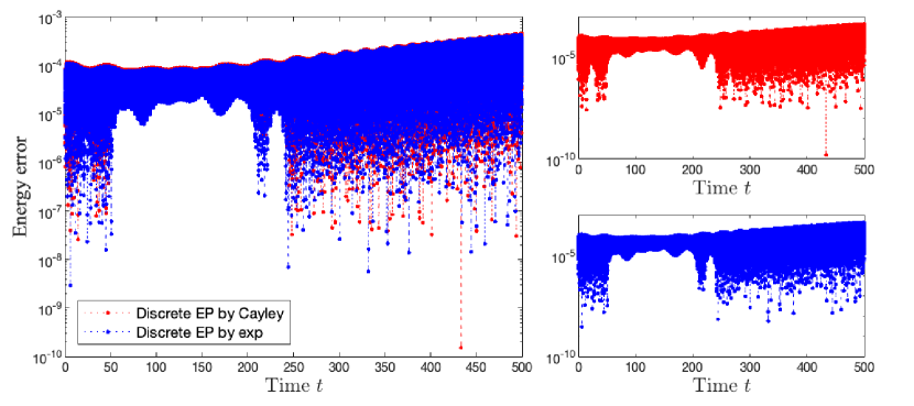
In the current setting, the underwater vehicle is influenced only by gravity and buoyancy forces and moments, with no other external forces acting on it, and hence the total energy is conserved. Figure 1 shows the relative error of energy over the time span of in a semi-logarithmic plot. The energy fluctuates within a certain range but tends to increase slightly over time. This is because of the Gauss–Newton method, which brings truncation errors.
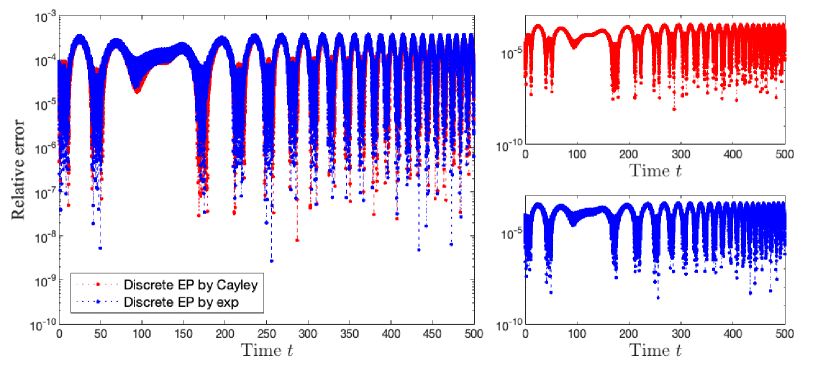
The time evolution of the Kelvin–Noether quantity, namely -component of the vector associated to given by (78) using the Lie algebra isomorphism (56), is shown in Figure 2 as a semi-logarithmic plot. Differences can hardly be observed in the two cases. Note that the Cayley transform is a second-order approximation of the matrix exponential [6].
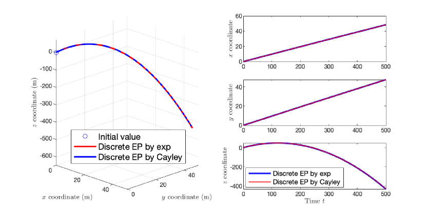
Given the current initial data and parameter settings, it is expected that the vehicle will initially rise due to the (positive) initial velocities and then descend under the combined effects of gravitational and buoyancy forces. Figure 3 confirms that the vehicle’s trajectories align with these expectations.
6 Conclusion
In this paper, we proposed the discrete Euler–Poincaré reduction for discrete Lagrangian systems on Lie groups with advected parameters and additional dynamics. The group difference map technique is employed to ensure that the trajectories remain in the configuration space, with the group difference map chosen as either the Cayley transform or the matrix exponential. Furthermore, we extended the Kelvin–Noether theorem to these systems in both the continuous and the discrete settings. These methods were applied to study the dynamics of underwater vehicles. We derived both the continuous and discrete Euler–Poincaré equations and performed numerical simulations based on the latter. The behavior of the conserved total energy and Kelvin–Noether quantity effectively illustrated the structure-preserving property of the scheme.
In future research, there remains significant scope for further exploration from both theoretical and applied perspectives. From a theoretical standpoint, it is important to extend the discrete Euler–Poincaré reduction for systems on finite-dimensional Lie groups with advected parameters and additional dynamics, as well as the corresponding Kelvin–Noether theorem, to infinite-dimensional Lie groups. This extension could lead to a more general framework that better captures the complexities of systems with infinite degrees of freedom, such as those arising in fluid dynamics or large-scale mechanical systems.
Furthermore, as illustrated in simulations of the underwater vehicle dynamics, the fluctuation of total energy increases due to the use of the Gauss–Newton method for the implicit scheme. This issue can be improved by using the moving frame method, which preserves total energy by maintaining the time-translational symmetry of the underlying variational problems, even in variational integration (e.g., [13, 32, 33]). It is important to note that in these numerical schemes, the time step often varies.
From an applied standpoint, fluid velocity and external forces in underwater vehicle dynamics should be further taken into account for real-world applications, such as control and path planning. The dynamics of underwater vehicles with fluid velocity has been modeled using the Lagrangian formulation (e.g., [1, 14]). However, the Euler–Poincaré reduction with additional dynamics has yet to be fully developed for this context. It is expected that fluid velocity can be included in the Lagrangian as an additional advected parameter. If a second advected parameter is introduced, the Kelvin–Noether theorem will be influenced by both advected parameters, and the associated Kelvin–Noether quantities may not be conserved in certain cases. It would also be interesting to generalize geometric optimal control strategies developed in, for example, [25, 28, 29], to invariant systems on Lie groups with advected parameters and additional dynamics using the Euler–Poincaré reduction. This would facilitate the extension of optimal control methods to underwater vehicle dynamics and other similar mechanical systems.
Acknowledgments
The authors are grateful to Darryl Holm, Ruiao Hu and Hiroaki Yoshimura for their inspiring discussions. YO is partially supported by JST SPRING (JPMJSP2123) and the Keio University Doctorate Student Grant-in-Aid Program from Ushioda Memorial Fund. LP is partially supported by JSPS KAKENHI (24K06852), JST CREST (JPMJCR1914, JPMJCR24Q5), and Keio University (Academic Development Fund, Fukuzawa Fund).
References
- [1] H. A. Ardakani. A variational principle for three-dimensional interactions between water waves and a floating rigid body with interior fluid motion. Journal of Fluid Mechanics, 866:630–659, 2019.
- [2] V. Arnold. Sur la géométrie différentielle des groupes de Lie de dimension infinie et ses applications à l’hydrodynamique des fluides parfaits. Annales de l’Institut Fourier, 16:319–361, 1966.
- [3] A. Bloch, P. Krishnaprasad, J. E. Marsden, and T. S. Ratiu. The Euler–Poincaré equations and double bracket dissipation. Communications in Mathematical Physics, 175:1–42, 1996.
- [4] A. I. Bobenko and Y. B. Suris. Discrete time Lagrangian mechanics on Lie groups, with an application to the Lagrange top. Communications in Mathematical Physics, 204:147–188, 1999.
- [5] N. Bou-Rabee and J. E. Marsden. Hamilton–Pontryagin integrators on Lie groups part I: Introduction and structure-preserving properties. Foundations of Computational Mathematics, 9:197–219, 2009.
- [6] N. M. Bou-Rabee. Hamilton–Pontryagin Integrators on Lie Groups. PhD thesis, California Institute of Technology, 2007.
- [7] H. Cendra, D. D. Holm, J. E. Marsden, and T. S. Ratiu. Lagrangian reduction, the Euler–Poincaré equations, and semidirect products. American Mathematical Society Translations, 186:1–25, 1998.
- [8] H. Cendra, J. E. Marsden, and T. S. Ratiu. Lagrangian Reduction by Stages. American Mathematical Society, Providence, 2001.
- [9] N. G. Chetayev. On the equations of Poincaré. Journal of Applied Mathematics and Mechanics, 5:253–262, 1941.
- [10] C. J. Cotter and D. D. Holm. On Noether’s theorem for the Euler–Poincaré equation on the diffeomorphism group with advected quantities. Foundations of Computational Mathematics, 13:457–477, 2013.
- [11] B. Couéraud and F. Gay-Balmaz. Variational discretization of thermodynamical simple systems on Lie groups. Discrete and Continuous Dynamical Systems - Series S, 13:1075–1102, 2020.
- [12] R. Cristi, F. A. Papoulias, and A. J. Healey. Adaptive sliding mode control of autonomous underwater vehicles in the dive plane. IEEE Journal of Oceanic Engineering, 15:152–160, 1990.
- [13] M. Fels and P. J. Olver. Moving coframes: II. Regularization and theoretical foundations. Acta Applicandae Mathematica, 55:127–208, 1999.
- [14] S. Fiori. Coordinate-free Lie-group-based modeling and simulation of a submersible vehicle. AIMS Mathematics, 9:10157–10184, 2024.
- [15] T. I. Fossen and O. E. Fjellstad. Nonlinear modelling of marine vehicles in 6 degrees of freedom. Mathematical Modelling of Systems, 1:17–27, 1995.
- [16] E. S. Gawlik, P. Mullen, D. Pavlov, J. E. Marsden, and M. Desbrun. Geometric, variational discretization of continuum theories. Physica D, 240:1724–1760, 2011.
- [17] Z. Ge and J. E. Marsden. Lie–Poisson Hamilton–Jacobi theory and Lie–Poisson integrators. Physics Letters A, 133:134–139, 1988.
- [18] G. Hamel. Die Lagrange–Eulerschen gleichungen der mechanik. Z. Mathematik und Physik, 50:1–57, 1904.
- [19] G. Hamel. Theoretische Mechanik. Springer-Verlag, Berlin, 1949.
- [20] D. D. Holm, R. Hu, and O. D. Street. Lagrangian reduction and wave mean flow interaction. Physica D, 454:133847, 2023.
- [21] D. D. Holm, J. E. Marsden, and T. S. Ratiu. The Euler–Poincaré equations and semidirect products with applications to continuum theories. Advances in Mathematics, 137:1–81, 1998.
- [22] D. D. Holm, J. E. Marsden, and T. S. Ratiu. The Euler–Poincaré equations in geophysical fluid dynamics. In Large-scale Atmosphere-Ocean Dynamics. II. Geometric Methods and Models, pages 251–299. Cambridge University Press, 2002.
- [23] D. D. Holm, T. Schmah, C. Stoica, and D. C. P. Ellis. Geometric Mechanics and Symmetry: From Finite to Infinite Dimensions. Oxford University Press, Oxford, 2009.
- [24] D. D. Holm and C. Tronci. Euler–Poincaré formulation of hybrid plasma models. Communications in Mathematical Sciences, 10:191–222, 2012.
- [25] I. I. Hussein, M. Leok, A. K. Sanyal, and A. M. Bloch. A discrete variational integrator for optimal control problems on . In Proceedings of the 45th IEEE Conference on Decision and Control, pages 6636–6641, 2006.
- [26] A. Iserles, H. Z. Munthe-Kaas, S. P. Nørsett, and A. Zanna. Lie-group methods. Acta Numerica, 9:215–365, 2000.
- [27] C. Kane, J. E. Marsden, M. Ortiz, and M. West. Variational integrators and the Newmark algorithm for conservative and dissipative mechanical systems. International Journal for Numerical Methods in Engineering, 49:1295–1325, 2000.
- [28] M. B. Kobilarov and J. E. Marsden. Discrete geometric optimal control on Lie groups. IEEE Transactions on Robotics, 27:641–655, 2011.
- [29] T. Lee, M. Leok, and N. H. McClamroch. Optimal attitude control of a rigid body using geometrically exact computations on . Journal of Dynamical and Control Systems, 14:465–487, 2008.
- [30] M. Leok. An overview of Lie group variational integrators and their applications to optimal control. In International Conference on Scientific Computation and Differential Equations. The French National Institute for Research in Computer Science and Control, 2007.
- [31] N. E. Leonard. Stability of a bottom-heavy underwater vehicle. Automatica, 33:331–346, 1997.
- [32] E. L. Mansfield. A Practical Guide to the Invariant Calculus. Cambridge University Press, Cambridge, 2010.
- [33] E. L. Mansfield, A. Rojo-Echeburúa, P. E. Hydon, and L. Peng. Moving frames and Noether’s finite difference conservation laws I. Transactions of Mathematics and Its Applications, 3:tnz004, 2019.
- [34] J. E. Marsden, S. Pekarsky, and S. Shkoller. Discrete Euler–Poincaré and Lie–Poisson equations. Nonlinearity, 12:1647, 1999.
- [35] J. E. Marsden and T. S. Ratiu. Introduction to Mechanics and Symmetry: A Basic Exposition of Classical Mechanical Systems. Springer, New York, 2nd edition, 2013.
- [36] J. E. Marsden, T. S. Ratiu, and J. Scheurle. Reduction theory and the Lagrange–Routh equations. Journal of Mathematical Physics, 41:3379–3429, 2000.
- [37] J. E. Marsden and J. Scheurle. Lagrangian reduction and the double spherical pendulum. Zeitschrift für Angewandte Mathematik und Physik ZAMP, 44:17–43, 1993.
- [38] J. E. Marsden and J. Scheurle. The reduced Euler–Lagrange equations. Fields Institute Communications, 1:139–164, 1993.
- [39] J. E. Marsden and M. West. Discrete mechanics and variational integrators. Acta Numerica, 10:357–514, 2001.
- [40] J. Moser and A. Veselov. Discrete versions of some classical integrable systems and factorization of matrix polynomials. Communications in Mathematical Physics, 139:217–243, 1991.
- [41] E. Noether. Invariante Variationsprobleme. Nachrichten von der Gesellschaft der Wissenschaften zu Göttingen, Mathematisch-Physikalische Klasse, 2:235–257, 1918.
- [42] N. Nordkvist and A. K. Sanyal. A Lie group variational integrator for rigid body motion in with applications to underwater vehicle dynamics. In 49th IEEE Conference on Decision and Control, pages 5414–5419, 2010.
- [43] P. J. Olver. Applications of Lie Groups to Differential Equations. Springer, New York, 2nd edition, 1993.
- [44] J. P. Panda, A. Mitra, and H. V. Warrior. A review on the hydrodynamic characteristics of autonomous underwater vehicles. Proceedings of the Institution of Mechanical Engineers, Part M: Journal of Engineering for the Maritime Environment, 235:15–29, 2021.
- [45] D. Pavlov, P. Mullen, Y. Tong, E. Kanso, J. E. Marsden, and M. Desbrun. Structure-preserving discretization of incompressible fluids. Physica D, 240:443–458, 2011.
- [46] L. Peng. Symmetries, conservation laws, and Noether’s theorem for differential-difference equations. Studies in Applied Mathematics, 139:457–502, 2017.
- [47] L. Peng and P. E. Hydon. Transformations, symmetries and Noether theorems for differential-difference equations. Proceedings of the Royal Society A: Mathematical, Physical and Engineering Sciences, 478:20210944, 2022.
- [48] H. Poincaré. Sur une forme nouvelle des équations de la mécanique. Comptes Rendus de l’Académie des Sciences de Paris, 132:369–371, 1901.
- [49] J. Squire, H. Qin, W. M. Tang, and C. Chandre. The Hamiltonian structure and Euler–Poincaré formulation of the Vlasov–Maxwell and gyrokinetic systems. Physics of Plasmas, 20, 2013.
- [50] A. P. Veselov. Integrable discrete-time systems and difference operators. Functional Analysis and Its Applications, 22:83–93, 1988.
- [51] J. M. Wendlandt and J. E. Marsden. Mechanical integrators derived from a discrete variational principle. Physica D, 106:223–246, 1997.