Polyspectral Mean Estimation of General Nonlinear Processes

Dhrubajyoti Ghoshlabel=e1 [    mark]dg302@duke.edu    Tucker McElroylabel=e2]tucker.s.mcelroy@census.gov [    Soumendra Lahirilabel=e3]s.lahiri@wustl.edu [ Department of Biostatistics and Bioinformatics, Duke University, Research and Methodology Directorate, U.S. Census Bureau, Department of Mathematics and Statistics, Washington University in St. Louis,
Abstract

Higher-order spectra (or polyspectra), defined as the Fourier Transform of a stationary process’ autocumulants, are useful in the analysis of nonlinear and non-Gaussian processes. Polyspectral means are weighted averages over Fourier frequencies of the polyspectra, and estimators can be constructed from analogous weighted averages of the higher-order periodogram (a statistic computed from the data sample’s discrete Fourier Transform). We derive the asymptotic distribution of a class of polyspectral mean estimators, obtaining an exact expression for the limit distribution that depends on both the given weighting function as well as on higher-order spectra. Secondly, we use bispectral means to define a new test of the linear process hypothesis. Simulations document the finite sample properties of the asymptotic results. Two applications illustrate our results’ utility: we test the linear process hypothesis for a Sunspot time series, and for the Gross Domestic Product we conduct a clustering exercise based on bispectral means with different weight functions.

Autocumulant,
Asymptotic normality,
Higher-order periodogram,
Linearity Testing,
Non-Gaussian Processes,
Polyspectral Density,
Time Series Clustering,
keywords:
\startlocaldefs\endlocaldefs\startlocaldefs\endlocaldefs

, , and

1 Introduction

Spectral Analysis is an important tool in time series analysis. The spectral density provides important insights into the underlying periodicities of a time series; see Brockwell, Davis [2016] and McElroy, Politis [2020]. However, when the stochastic process is nonlinear, higher-order autocumulants (cf. Brillinger [2001]) can furnish valuable insights that are not discernible from the spectral density, as argued in Brillinger, Rosenblatt [1967]. In particular, three- and four-way interactions of a nonlinear process can be measured through the third and fourth order polyspectra; see Brillinger [1965], Brillinger, Rosenblatt [1967], Brockett et al. [1988], Gabr [1988], Maravall [1983], Mendel [1991], and Berg, Politis [2009]. Linear functionals of higher-order spectra (here referred to as polyspectral means) are often encountered in the analysis of nonlinear time series, and are therefore a serious object of inference. Whereas there is an existent literature on estimation of polyspectra (Brillinger, Rosenblatt [1967], Van Ness [1966], Raghuveer, Nikias [1986], Spooner, Gardner [1991]), inference for polyspectral means remains a gap. This paper aims to fill this gap by developing asymptotic distributional results on polyspectral means, and by developing statistical inference methodology for nonlinear time series analysis.

Let {Xt}subscript𝑋𝑡\{X_{t}\} be a (k+1)thsuperscript𝑘1𝑡(k+1)^{th} order stationary time series, that is, E[|Xt|k+1]<𝐸delimited-[]superscriptsubscript𝑋𝑡𝑘1E[{|X_{t}|}^{k+1}]<\infty and
EXtXt+h1Xt+hr=EX1X1+h1X1+hr𝐸subscript𝑋𝑡subscript𝑋𝑡subscript1subscript𝑋𝑡subscript𝑟𝐸subscript𝑋1subscript𝑋1subscript1subscript𝑋1subscript𝑟EX_{t}X_{t+h_{1}}\ldots X_{t+h_{r}}=EX_{1}X_{1+h_{1}}\ldots X_{1+h_{r}} for all integers t,h1,,hr𝑡subscript1subscript𝑟t,h_{1},\ldots,h_{r}, and for all 1rk1𝑟𝑘1\leq r\leq k, for given k1𝑘1k\geq 1. The most commonly occurring case is k=1𝑘1k=1, corresponding to the class of second order stationary (SOS) processes. Thus, for a SOS process {Xt}subscript𝑋𝑡\{X_{t}\}, EXt=EX1𝐸subscript𝑋𝑡𝐸subscript𝑋1EX_{t}=EX_{1} is a constant and its cross-covariances depend only on the time-difference Cov(Xt,Xt+h)=γ(h)Covsubscript𝑋𝑡subscript𝑋𝑡𝛾\mbox{Cov}(X_{t},X_{t+h})=\gamma(h) for all t,h𝑡t,h\in{\mathbb{Z}}, where ={0,±1,±2,}0plus-or-minus1plus-or-minus2{\mathbb{Z}}=\{0,\pm 1,\pm 2,\ldots\} denotes the set of all integers. When the autocovariance function γ(h)γh𝛾subscript𝛾\gamma(h)\equiv\gamma_{h} is absolutely summable, {Xt}subscript𝑋𝑡\{X_{t}\} has a spectral density given by f(λ)=hγ(h)eιhλ𝑓𝜆subscript𝛾superscript𝑒𝜄𝜆f(\lambda)=\sum_{h\in{\mathbb{Z}}}\gamma(h)e^{-{\iota}h\lambda}, λ[π,π]𝜆𝜋𝜋\lambda\in[-\pi,\pi], where ι=1𝜄1{\iota}=\sqrt{-1}.

Important features of a stochastic process can be extracted with a spectral mean, which is defined as [π,π]f(λ)g(λ)𝑑λsubscript𝜋𝜋𝑓𝜆𝑔𝜆differential-d𝜆\int_{[-\pi,\pi]}f(\lambda)g(\lambda)d\lambda, where g()𝑔g(\cdot) is a weight function. Spectral means can provide important insights into the time series afforded by different g functions. For example, a spectral mean with g(λ)=cos(hλ)𝑔𝜆𝑐𝑜𝑠𝜆g(\lambda)=cos(h\lambda) corresponds to the lag hh autocovariance, whereas g(λ)=11(a,a)𝑔𝜆11𝑎𝑎g(\lambda)={1\!\!1}(-a,a) gives the spectral content in the interval (a,a)𝑎𝑎(-a,a), where 11()11{1\!\!1}(\cdot) denotes the indicator function. Analogous definitions can be made for higher order spectra. The (k+1)thsuperscript𝑘1𝑡(k+1)^{th} order autocumulant is defined as γ(h1,,hk)=Cum(Xt,Xt+h1,,Xt+hk)𝛾subscript1subscript𝑘Cumsubscript𝑋𝑡subscript𝑋𝑡subscript1subscript𝑋𝑡subscript𝑘\gamma(h_{1},\ldots,h_{k})=\mbox{Cum}(X_{t},X_{t+h_{1}},\ldots,X_{t+h_{k}}) for all t𝑡t, where Cum(X,Y,,Z)Cum𝑋𝑌𝑍\mbox{Cum}(X,Y,\ldots,Z) denotes the cumulant of jointly distributed random variables {X,Y,,Z}𝑋𝑌𝑍\{X,Y,\ldots,Z\} (cf. Brillinger [2001]) and where h1,,hksubscript1subscript𝑘h_{1},\ldots,h_{k} are integer lags. If the corresponding autocumulant function is absolutely summable, then we define the polyspectra of order k𝑘k as the Fourier transform of the (k+1)thsuperscript𝑘1𝑡(k+1)^{th} order autocumulants:

fk(λ¯)=h¯kγ(h¯)eιh¯λ¯,subscript𝑓𝑘¯𝜆subscript¯superscript𝑘𝛾¯superscript𝑒𝜄superscript¯¯𝜆f_{k}(\underline{\lambda})=\sum_{\underline{h}\in{\mathbb{Z}}^{k}}\gamma(\underline{h})e^{-\iota\underline{h}^{\prime}\underline{\lambda}}\,,

where h¯=[h1,,hk]¯superscriptsubscript1subscript𝑘\underline{h}={[h_{1},\ldots,h_{k}]}^{\prime}, λ¯=[λ1,,λk]¯𝜆superscriptsubscript𝜆1subscript𝜆𝑘\underline{\lambda}={[\lambda_{1},\ldots,\lambda_{k}]}^{\prime} and Asuperscript𝐴A^{\prime} denotes the transpose of a matrix A𝐴A. A polyspectral mean with weight function g:[π,π]k:𝑔superscript𝜋𝜋𝑘g:[-\pi,\pi]^{k}\rightarrow\mathbb{C} is defined as

Mg(fk)=[π,π]kfk(λ¯)g(λ¯)𝑑λ¯.subscript𝑀𝑔subscript𝑓𝑘subscriptsuperscript𝜋𝜋𝑘subscript𝑓𝑘¯𝜆𝑔¯𝜆differential-d¯𝜆M_{g}(f_{k})=\int_{[-\pi,\pi]^{k}}f_{k}(\underline{\lambda})g(\underline{\lambda})d\underline{\lambda}. (1.1)

Thus, spectral means correspond to the case k=1𝑘1k=1, in which case we drop the subscript k𝑘k (and write f1=fsubscript𝑓1𝑓f_{1}=f). Polyspectral means give us important information about a time series that can not be obtained from the spectral distribution, e.g., when the time series is nonlinear or the innovation process is non-Gaussian. Additionally, we can extract several features from a time series through the polyspectral mean corresponding to different weight functions. These features can play an important role in identifying (dis-)similarities among different time series (cf. Chua et al. [2010], Picinbono [1999], Dubnov [1996], Vrabie et al. [2003]).
Refer to caption
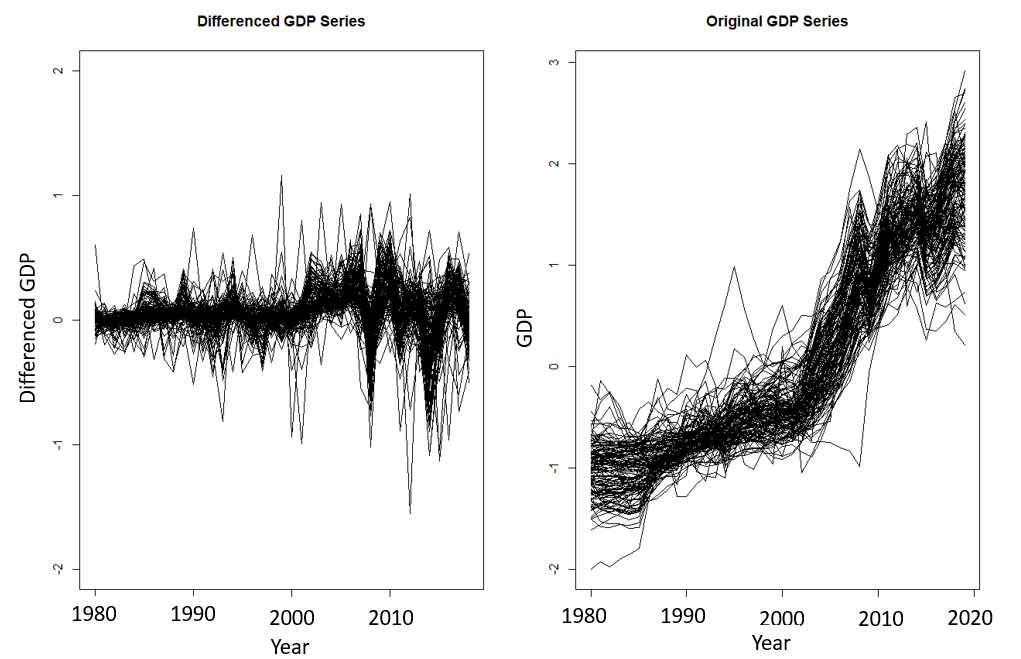
Figure 1: Differenced GDP (left panel) and raw GDP (right panel) for 136 countries, annual 1980-2020. There is a common nonlinear trend (right panel).

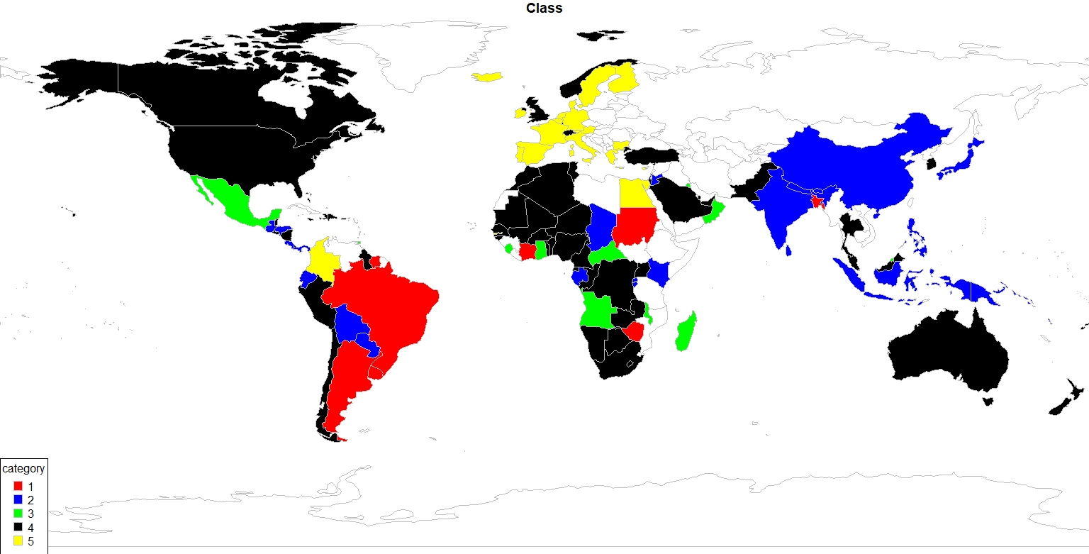
For an illustrative example, we consider the annual Gross Domestic Product (GDP) data from 136 countries over 40 years. Our goal is to obtain clustering of the countries based on patterns of their GDP growth rates. The right panel of Figure 1 gives the raw time series and the left panel gives the differenced and scaled versions of the GDP of different countries. As a part of exploratory data analysis, we tested for Gaussianity and linearity; a substantial proportion of the time series are non-Gaussian, and some of them are nonlinear. Hence, using spectral means alone to capture relevant time series features may be inadequate. Here we use (estimated) higher order polyspectral means with different weight functions to elicit salient features of the GDP data, in order to capture possible nonlinear dynamics of the economies. See Section 6 for more details.

Estimation of spectral and polyspectral means can be carried out using the periodogram and its higher order versions, which are defined in terms of the discrete Fourier transform of a length T𝑇T sample {X1,,XT}subscript𝑋1subscript𝑋𝑇\{X_{1},\ldots,X_{T}\} (described in Section 2). However, distributional properties of the polyspectral mean estimators are not very well-studied. Dahlhaus [1985] proved the asymptotic normality of spectral means, i.e., the case k=1𝑘1k=1; however, in the general case (k>1𝑘1k>1), there does not seem to be any work on the asymptotic distribution of polyspectral mean estimators. One of the major contributions of this paper is to establish asymptotic normality results for the polyspectral means of a general order. We develop some nontrivial combinatorial arguments involving higher-order autocumulants to show that, under mild conditions, the estimators of the kthsuperscript𝑘𝑡k^{th} order polyspectral mean parameter Mg(fk)subscript𝑀𝑔subscript𝑓𝑘M_{g}(f_{k}) in (1.1) are asymptotically normal. We also obtain an explicit expression for the asymptotic variance, which is shown to depend on certain polyspectral means of order 2k+12𝑘12k+1. This result agrees with the known results on spectral means when specialized to the case k=1𝑘1k=1, where the limiting variance is known to involve the trispectrum f2k+1=f3subscript𝑓2𝑘1subscript𝑓3f_{2k+1}=f_{3}. In particular, the results of this paper provide a unified way to construct studentized versions of spectral mean estimators and higher order polyspectral mean estimators, which can be used to carry out large sample statistical inference on polyspectral mean parameters of any arbitrary order k1𝑘1k\geq 1.

The second major contribution of the paper is the development of a new test procedure to assess the linearity assumption on a time series. Earlier work on the problem is typically based on the squared modulus of the estimated bispectrum (Rao, Gabr [1980], Chan, Tong [1986], Berg et al. [2010], Barnett, Wolff [2004]). In contrast, here we make a key observation that under the linearity hypothesis (i.e., the null hypothesis) the ratio of the bispectrum to a suitable power transformation of the spectral density must be a constant at all frequency pairs in [π,π]2superscript𝜋𝜋2[-\pi,\pi]^{2}. This observation allows us to construct a set of higher order polyspectral means that must be zero when the process is linear. On the other hand, for a nonlinear process, not all of these spectral means can be equal to zero. Here we exploit this fact and develop a new test statistic that can be used to test the significance of these polyspectral means. We also derive the asymptotic distribution of the test statistic under the null hypothesis, and provide the critical values needed for calibrating the proposed test.

The rest of the paper is organized as follows. Section 2 covers some background material, and provides some examples of polyspectra and polyspectral means. Section 3 gives the regularity conditions and the asymptotic properties of the polyspectral means of a general order. The linearity test is described in Section 4. Simulations are presented in Section 5, and two data applications, one involving the Sunspot data and the other involving the GDP growth rate (with a discussion of clustering time series via bispectral means), are presented in Section 6. The proofs of the theoretical results are given in Section 7.

2 Background and examples

First, we will define estimators of the polyspectral mean Mg(fk)subscript𝑀𝑔subscript𝑓𝑘M_{g}\left(f_{k}\right) defined in (1.1), corresponding to a given weight function g𝑔g. Following Brillinger, Rosenblatt [1967], we define an estimator of Mg(fk)subscript𝑀𝑔subscript𝑓𝑘M_{g}\left(f_{k}\right) by replacing fksubscript𝑓𝑘f_{k} by the kthsuperscript𝑘𝑡k^{th} order periodogram. Specifically, given a sample {X1,,XT}subscript𝑋1subscript𝑋𝑇\{X_{1},\ldots,X_{T}\} from the mean zero time series {Xt}subscript𝑋𝑡\{X_{t}\}, let d(λ)=t=1TXteιλt𝑑𝜆superscriptsubscript𝑡1𝑇subscript𝑋𝑡superscript𝑒𝜄𝜆𝑡d(\lambda)=\sum_{t=1}^{T}X_{t}e^{-\iota\lambda t} denote the Discrete Fourier Transform (DFT) of the sample, where λ(π,π]𝜆𝜋𝜋\lambda\in(-\pi,\pi] and ι=1𝜄1\iota=\sqrt{-1}. Such a frequency may be a Fourier frequency, taking the form 2π/T2𝜋𝑇2\pi\ell/T for some integer {T2,,T2}𝑇2𝑇2\ell\in\{-\lfloor\frac{T}{2}\rfloor,\ldots,\lfloor\frac{T}{2}\rfloor\}, in which case we write λ~~𝜆\tilde{\lambda}. Here and in the following, x𝑥\lfloor x\rfloor denotes the integer part of a real number x𝑥x. A k𝑘k-vector of frequencies is denoted by λ¯=[λ1,,λk]¯𝜆superscriptsubscript𝜆1subscript𝜆𝑘\underline{\lambda}={[\lambda_{1},\ldots,\lambda_{k}]}^{\prime}; if these are all Fourier frequencies, then we write λ¯~~¯𝜆\tilde{\underline{\lambda}}. Then the kthsuperscript𝑘𝑡k^{th} order periodogram is defined as

f^k(λ¯)=T1d(λ1)d(λk)d([λ¯]),subscript^𝑓𝑘¯𝜆superscript𝑇1𝑑subscript𝜆1𝑑subscript𝜆𝑘𝑑delimited-[]¯𝜆\hat{f}_{k}(\underline{\lambda})=T^{-1}d(\lambda_{1})\cdots d(\lambda_{k})d(-[\underline{\lambda}]),

where [λ¯]delimited-[]¯𝜆[\underline{\lambda}] is a shorthand for j=1kλjsuperscriptsubscript𝑗1𝑘subscript𝜆𝑗\sum_{j=1}^{k}\lambda_{j}. Next, let λ¯~subscript~¯𝜆\sum_{\tilde{\underline{\lambda}}} denote a shorthand for a summation over vector λ¯¯𝜆\underline{\lambda} that consist of Fourier frequencies. Then we define the estimator of the polyspectral mean Mg(fk)subscript𝑀𝑔subscript𝑓𝑘M_{g}\left(f_{k}\right) as

Mg(fk)^^subscript𝑀𝑔subscript𝑓𝑘\displaystyle\widehat{M_{g}(f_{k})} (2π)kTkλ¯~f^k(λ¯~)g(λ¯~)Φ(λ¯~)absentsuperscript2𝜋𝑘superscript𝑇𝑘subscript~¯𝜆subscript^𝑓𝑘~¯𝜆𝑔~¯𝜆Φ~¯𝜆\displaystyle\equiv(2\pi)^{k}T^{-k}\sum_{\tilde{\underline{\lambda}}}\hat{f}_{k}(\tilde{\underline{\lambda}})g\left(\tilde{\underline{\lambda}}\right)\Phi(\tilde{\underline{\lambda}})
=(2π)kTk1λ¯~d(λ1~)d(λk~)d([λ¯~])g(λ¯~)Φ(λ¯~),absentsuperscript2𝜋𝑘superscript𝑇𝑘1subscript~¯𝜆𝑑~subscript𝜆1𝑑~subscript𝜆𝑘𝑑delimited-[]~¯𝜆𝑔~¯𝜆Φ~¯𝜆\displaystyle=(2\pi)^{k}T^{-k-1}\sum_{\tilde{\underline{\lambda}}}d\left(\tilde{\lambda_{1}}\right)\cdots d\left(\tilde{\lambda_{k}}\right)d\left(-[\tilde{\underline{\lambda}}]\right)g\left(\tilde{\underline{\lambda}}\right)\Phi(\tilde{\underline{\lambda}}), (2.1)

where Φ(λ¯)Φ¯𝜆\Phi(\underline{\lambda}) is an indicator function that is zero if and only if λ¯¯𝜆\underline{\lambda} lies in any proper linear sub-manifold of the k𝑘k-torus [π,π]ksuperscript𝜋𝜋𝑘{[-\pi,\pi]}^{k}. That is, Φ(λ¯)Φ¯𝜆\Phi(\underline{\lambda}) is one if and only if for all subset λi1,,λimsubscript𝜆subscript𝑖1subscript𝜆subscript𝑖𝑚\lambda_{i_{1}},\ldots,\lambda_{i_{m}} of λ¯¯𝜆\underline{\lambda} (1mk1𝑚𝑘1\leq m\leq k), j=1mλij0 (mod 2π)\sum_{j=1}^{m}\lambda_{i_{j}}\not\equiv 0\textrm{ (mod }2\pi). We further assume that the weighting function g𝑔g is continuous in λ¯¯𝜆\underline{\lambda} (except possibly on a set of Lebesgue measure zero; cf. Section 2.4, Athreya, Lahiri [2006] ), and satisfies the symmetry condition

g(λ¯)=g(λ¯)¯𝑔¯𝜆¯𝑔¯𝜆g(\underline{\lambda})=\overline{g(-\underline{\lambda})} (2.2)

for all λ¯¯𝜆\underline{\lambda}. This condition holds for all polyspectra, and holds more broadly for any function that has a multi-variable Fourier expansion with real coefficients, thereby encompassing most functions of interest in applications. Moreover, this assumption ensures that the corresponding polyspectral mean is real-valued, since

Mg(fk)¯=[π,π]kfk(λ¯)¯g(λ¯)¯𝑑λ¯=[π,π]kfk(λ¯)g(λ¯)𝑑λ¯=Mg(fk),¯subscript𝑀𝑔subscript𝑓𝑘subscriptsuperscript𝜋𝜋𝑘¯subscript𝑓𝑘¯𝜆¯𝑔¯𝜆differential-d¯𝜆subscriptsuperscript𝜋𝜋𝑘subscript𝑓𝑘¯𝜆𝑔¯𝜆differential-d¯𝜆subscript𝑀𝑔subscript𝑓𝑘\overline{M_{g}(f_{k})}=\int_{[-\pi,\pi]^{k}}\overline{f_{k}(\underline{\lambda})}\overline{g(\underline{\lambda})}\,d\underline{\lambda}=\int_{[-\pi,\pi]^{k}}f_{k}(-\underline{\lambda})g(-\underline{\lambda})\,d\underline{\lambda}=M_{g}(f_{k}),

using (2.2) and a change of variable λ¯λ¯maps-to¯𝜆¯𝜆-\underline{\lambda}\mapsto\underline{\lambda}. We will also assume that λ¯|g(λ¯)|<subscript¯𝜆𝑔¯𝜆\int_{\underline{\lambda}}\lvert g\left(\underline{\lambda}\right)\rvert<\infty, which screens out perverse cases of that are of little practical interest.

Note that the value of the polyspectral mean (1.1) is the same whether or not we restrict integration to sub-manifolds of the torus, since such sets have Lebesgue measure zero. We need to introduce the indicator function, since Brillinger, Rosenblatt [1967] established that the kthsuperscript𝑘𝑡k^{th} order periodogram diverges if the Fourier frequencies lie in such sub-manifolds. This is a significant issue. Indeed, the estimator of the polyspectral density in Brillinger [1965] is also given by a kernel-weighted average of the kthsuperscript𝑘𝑡k^{th} order periodogram, where the average is taken by avoiding the sub-manifolds. The polyspectral density estimator involves a bandwidth term, which in general makes the convergence rate much slower. Since we are working with polyspectral means, it is not necessary to smooth the kthsuperscript𝑘𝑡k^{th} order periodogram, and hence we can ignore the bandwidth problem and focus directly on regions that avoid the sub-manifolds.
Refer to caption
Refer to caption
Refer to caption
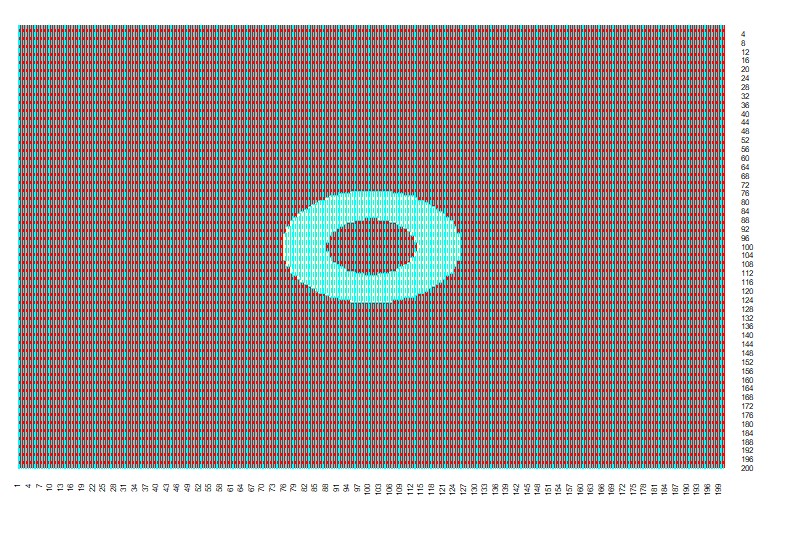
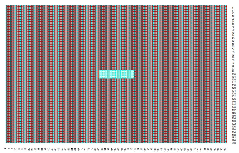
Figure 2: Heatmap for different g functions: (left panel) g(λ¯)=cos(2λ)cos(3λ)𝑔¯𝜆𝑐𝑜𝑠2𝜆𝑐𝑜𝑠3𝜆g(\underline{\lambda})=cos(2\lambda)cos(3\lambda), (center panel) g(λ¯)=𝕀(λ10.2)𝕀(λ20.2)𝑔¯𝜆𝕀subscript𝜆10.2𝕀subscript𝜆20.2g(\underline{\lambda})=\mathbb{I}(\lambda_{1}\leq 0.2)\mathbb{I}(\lambda_{2}\leq 0.2), (right panel) g(λ¯)=𝕀(0.1λ12+λ220.2)𝑔¯𝜆𝕀0.1superscriptsubscript𝜆12superscriptsubscript𝜆220.2g(\underline{\lambda})=\mathbb{I}(0.1\leq\lambda_{1}^{2}+\lambda_{2}^{2}\leq 0.2).

Some illustrations of weighting functions are given in Figure 2. We also provide some specific examples of polyspectral means below, demonstrating how diverse features of a nonlinear process can be extracted with different weighting functions. (Recall that we assumed that the process has mean zero, which assumption is used throughout.)

Example 2.1 (Example 1:).

Our first example, which was mentioned in the introduction, is already familiar: let g(λ1)=(2π)1exp{ιλ1h1}𝑔subscript𝜆1superscript2𝜋1𝜄subscript𝜆1subscript1g(\lambda_{1})={(2\pi)}^{-1}\exp\{\iota\lambda_{1}h_{1}\}, so that Mg(f1)=ππf1(λ1)g(λ1)𝑑λ1=γ(h1)subscript𝑀𝑔subscript𝑓1superscriptsubscript𝜋𝜋subscript𝑓1subscript𝜆1𝑔subscript𝜆1differential-dsubscript𝜆1𝛾subscript1M_{g}(f_{1})=\int_{-\pi}^{\pi}f_{1}(\lambda_{1})g(\lambda_{1})d\lambda_{1}=\gamma(h_{1}), where γ()𝛾\gamma(\cdot) is the second order autocumulant function, i.e., the autocovariance function. Its classical estimator is the sample autocovariance γ^(h1)=T1tXtXt+h1^𝛾subscript1superscript𝑇1subscript𝑡subscript𝑋𝑡subscript𝑋𝑡subscript1\hat{\gamma}(h_{1})=T^{-1}\sum_{t}X_{t}X_{t+h_{1}}, where the summation is over all t𝑡t such that t,t+h1{1,2,,T}𝑡𝑡subscript112𝑇t,t+h_{1}\in\{1,2,\ldots,T\} (the sampling times). This agrees with our proposed polyspectral mean estimator, viz. Mg(f1)^=T2λ1~d(λ1~)d(λ1~)g(λ1~)=γ^(h1)^subscript𝑀𝑔subscript𝑓1superscript𝑇2subscript~subscript𝜆1𝑑~subscript𝜆1𝑑~subscript𝜆1𝑔~subscript𝜆1^𝛾subscript1\widehat{M_{g}(f_{1})}=T^{-2}\sum_{\tilde{\lambda_{1}}}d(\tilde{\lambda_{1}})d(-\tilde{\lambda_{1}})g(\tilde{\lambda_{1}})=\hat{\gamma}(h_{1}), using the fact that

λ1~exp{ιλ1~s}=T 11{s=0}.subscript~subscript𝜆1𝜄~subscript𝜆1𝑠𝑇1subscript1𝑠0\sum_{\tilde{\lambda_{1}}}\exp\{\iota\tilde{\lambda_{1}}s\}=T\,{1\!\!1}_{\{s=0\}}. (2.3)

Note that in our expression for Mg(f1)^^subscript𝑀𝑔subscript𝑓1\widehat{M_{g}(f_{1})} there are no sub-manifolds of the 1-torus.

Example 1 can be extended to third-order autocumulants via the weight function g(λ1,λ2)=(2π)2exp{ιλ1h1+ιλ2h2}𝑔subscript𝜆1subscript𝜆2superscript2𝜋2𝜄subscript𝜆1subscript1𝜄subscript𝜆2subscript2g(\lambda_{1},\lambda_{2})={(2\pi)}^{-2}\exp\{\iota\lambda_{1}h_{1}+\iota\lambda_{2}h_{2}\}. Then it follows that

Mg(f2)=ππππf2(λ¯)g(λ¯)𝑑λ¯=γ(h1,h2),subscript𝑀𝑔subscript𝑓2superscriptsubscript𝜋𝜋superscriptsubscript𝜋𝜋subscript𝑓2¯𝜆𝑔¯𝜆differential-d¯𝜆𝛾subscript1subscript2M_{g}(f_{2})=\int_{-\pi}^{\pi}\int_{-\pi}^{\pi}f_{2}(\underline{\lambda})g(\underline{\lambda})d\underline{\lambda}=\gamma(h_{1},h_{2}), (2.4)

where γ(,)𝛾\gamma(\cdot,\cdot) is the third order autocumulant function. The classical estimator of this autocumulant function is given by γ^(h1,h2)=T1tXtXt+h1Xt+h2,^𝛾subscript1subscript2superscript𝑇1subscript𝑡subscript𝑋𝑡subscript𝑋𝑡subscript1subscript𝑋𝑡subscript2\hat{\gamma}(h_{1},h_{2})=T^{-1}\sum_{t}X_{t}X_{t+h_{1}}X_{t+h_{2}}, where the summation is over all t𝑡t such that t,t+h1,t+h2{1,2,,T}𝑡𝑡subscript1𝑡subscript212𝑇t,t+h_{1},t+h_{2}\in\{1,2,\ldots,T\}. We next show that this is asymptotically equivalent (i.e., the same up to terms tending to zero in probability) to Mg(f2)^^subscript𝑀𝑔subscript𝑓2\widehat{M_{g}(f_{2})}. First, note that the sub-manifolds of the 2-torus that we must exclude are simply the sets where either λ~1subscript~𝜆1\tilde{\lambda}_{1} or λ~2subscript~𝜆2\tilde{\lambda}_{2} equals zero; hence

Mg(f2)^^subscript𝑀𝑔subscript𝑓2\displaystyle\widehat{M_{g}(f_{2})} =T3λ1~,λ2~0d(λ1~)d(λ2~)d(λ1~λ2~)eιλ1~h1+ιλ2~h2absentsuperscript𝑇3subscript~subscript𝜆1~subscript𝜆20𝑑~subscript𝜆1𝑑~subscript𝜆2𝑑~subscript𝜆1~subscript𝜆2superscript𝑒𝜄~subscript𝜆1subscript1𝜄~subscript𝜆2subscript2\displaystyle=T^{-3}\sum_{\tilde{\lambda_{1}},\tilde{\lambda_{2}}\neq 0}d(\tilde{\lambda_{1}})d(\tilde{\lambda_{2}})d(-\tilde{\lambda_{1}}-\tilde{\lambda_{2}})e^{\iota\tilde{\lambda_{1}}h_{1}+\iota\tilde{\lambda_{2}}h_{2}}
=T3λ1~,λ2~t1,t2,t3Xt1Xt2Xt3eιλ1~t1eιλ2~t2eι(λ1~+λ2~)t3eιλ1~h1eιλ2~h2absentsuperscript𝑇3subscript~subscript𝜆1~subscript𝜆2subscriptsubscript𝑡1subscript𝑡2subscript𝑡3subscript𝑋subscript𝑡1subscript𝑋subscript𝑡2subscript𝑋subscript𝑡3superscript𝑒𝜄~subscript𝜆1subscript𝑡1superscript𝑒𝜄~subscript𝜆2subscript𝑡2superscript𝑒𝜄~subscript𝜆1~subscript𝜆2subscript𝑡3superscript𝑒𝜄~subscript𝜆1subscript1superscript𝑒𝜄~subscript𝜆2subscript2\displaystyle=T^{-3}\sum_{\tilde{\lambda_{1}},\tilde{\lambda_{2}}}\sum_{t_{1},t_{2},t_{3}}X_{t_{1}}X_{t_{2}}X_{t_{3}}e^{-\iota\tilde{\lambda_{1}}t_{1}}e^{-\iota\tilde{\lambda_{2}}t_{2}}e^{\iota(\tilde{\lambda_{1}}+\tilde{\lambda_{2}})t_{3}}e^{\iota\tilde{\lambda_{1}}h_{1}}e^{\iota\tilde{\lambda_{2}}h_{2}}
T3λ1~t1,t2,t3Xt1Xt2Xt3eιλ1~(t3t1+h1)T3λ2~t1,t2,t3Xt1Xt2Xt3eιλ2~(t3t2+h2)superscript𝑇3subscript~subscript𝜆1subscriptsubscript𝑡1subscript𝑡2subscript𝑡3subscript𝑋subscript𝑡1subscript𝑋subscript𝑡2subscript𝑋subscript𝑡3superscript𝑒𝜄~subscript𝜆1subscript𝑡3subscript𝑡1subscript1superscript𝑇3subscript~subscript𝜆2subscriptsubscript𝑡1subscript𝑡2subscript𝑡3subscript𝑋subscript𝑡1subscript𝑋subscript𝑡2subscript𝑋subscript𝑡3superscript𝑒𝜄~subscript𝜆2subscript𝑡3subscript𝑡2subscript2\displaystyle-T^{-3}\sum_{\tilde{\lambda_{1}}}\sum_{t_{1},t_{2},t_{3}}X_{t_{1}}X_{t_{2}}X_{t_{3}}e^{\iota\tilde{\lambda_{1}}(t_{3}-t_{1}+h_{1})}-T^{-3}\sum_{\tilde{\lambda_{2}}}\sum_{t_{1},t_{2},t_{3}}X_{t_{1}}X_{t_{2}}X_{t_{3}}e^{\iota\tilde{\lambda_{2}}(t_{3}-t_{2}+h_{2})}
+T3t1,t2,t3Xt1Xt2Xt3.superscript𝑇3subscriptsubscript𝑡1subscript𝑡2subscript𝑡3subscript𝑋subscript𝑡1subscript𝑋subscript𝑡2subscript𝑋subscript𝑡3\displaystyle+T^{-3}\sum_{t_{1},t_{2},t_{3}}X_{t_{1}}X_{t_{2}}X_{t_{3}}.

Note that the last term is simply the cube of the sample mean X¯¯𝑋\overline{X}, which tends to zero in probability. For the other terms, we can apply (2.3) to obtain Mg(f2)^=T1t1Xt1Xt1+h1Xt1+h2T1t2Xt2T1t1Xt1Xt1h1T1t1Xt1T1t2Xt2Xt2h2+(X¯)3^subscript𝑀𝑔subscript𝑓2superscript𝑇1subscriptsubscript𝑡1subscript𝑋subscript𝑡1subscript𝑋subscript𝑡1subscript1subscript𝑋subscript𝑡1subscript2superscript𝑇1subscriptsubscript𝑡2subscript𝑋subscript𝑡2superscript𝑇1subscriptsubscript𝑡1subscript𝑋subscript𝑡1subscript𝑋subscript𝑡1subscript1superscript𝑇1subscriptsubscript𝑡1subscript𝑋subscript𝑡1superscript𝑇1subscriptsubscript𝑡2subscript𝑋subscript𝑡2subscript𝑋subscript𝑡2subscript2superscript¯𝑋3\widehat{M_{g}(f_{2})}=T^{-1}\sum_{t_{1}}X_{t_{1}}X_{t_{1}+h_{1}}X_{t_{1}+h_{2}}-T^{-1}\sum_{t_{2}}X_{t_{2}}T^{-1}\sum_{t_{1}}X_{t_{1}}X_{t_{1}-h_{1}}-T^{-1}\sum_{t_{1}}X_{t_{1}}T^{-1}\sum_{t_{2}}X_{t_{2}}X_{t_{2}-h_{2}}+{(\overline{X})}^{3}, which is asymptotically equivalent to γ^(h1,h2)^𝛾subscript1subscript2\hat{\gamma}(h_{1},h_{2}).

Example 2.2 (Example 2:).

For a zero mean process, the autocumulants and automoments of order 2 and 3 coincide, and therefore Example 1 shows that the spectral mean estimator is a consistent estimator of these autocumulants/automoments. A similar (but more involved) calculation is required to show that a similar result holds for higher order autocumulants. As an example, we now consider the fourth order autocumulant function (which is different from the fourth order automoment function). To that end, we consider the trispectral mean with the weight function g(λ1,λ2,λ3)=(2π)3exp{ι(λ1h1+λ2h2+λ3h3)}𝑔subscript𝜆1subscript𝜆2subscript𝜆3superscript2𝜋3𝜄subscript𝜆1subscript1subscript𝜆2subscript2subscript𝜆3subscript3g(\lambda_{1},\lambda_{2},\lambda_{3})={(2\pi)}^{-3}\exp\{\iota(\lambda_{1}h_{1}+\lambda_{2}h_{2}+\lambda_{3}h_{3})\}. Then, letting η(k1,k2,k3)𝜂subscript𝑘1subscript𝑘2subscript𝑘3\eta(k_{1},k_{2},k_{3}) denote the order 3 auto-moment, and using the identity γ(k1,k2,k3)=η(k1,k2,k3)γ(k1)γ(k3k2)γ(k2)γ(k3k1)γ(k3)γ(k2k1)𝛾subscript𝑘1subscript𝑘2subscript𝑘3𝜂subscript𝑘1subscript𝑘2subscript𝑘3𝛾subscript𝑘1𝛾subscript𝑘3subscript𝑘2𝛾subscript𝑘2𝛾subscript𝑘3subscript𝑘1𝛾subscript𝑘3𝛾subscript𝑘2subscript𝑘1\gamma(k_{1},k_{2},k_{3})=\eta(k_{1},k_{2},k_{3})-\gamma(k_{1})\gamma(k_{3}-k_{2})-\gamma(k_{2})\gamma(k_{3}-k_{1})-\gamma(k_{3})\gamma(k_{2}-k_{1}), we get

Mg(f3)subscript𝑀𝑔subscript𝑓3\displaystyle M_{g}(f_{3}) =(8π3)1ππππππk1,k2,k3γ(k1,k2,k3)absentsuperscript8superscript𝜋31superscriptsubscript𝜋𝜋superscriptsubscript𝜋𝜋superscriptsubscript𝜋𝜋subscriptsubscript𝑘1subscript𝑘2subscript𝑘3𝛾subscript𝑘1subscript𝑘2subscript𝑘3\displaystyle=(8\pi^{3})^{-1}\int_{-\pi}^{\pi}\int_{-\pi}^{\pi}\int_{-\pi}^{\pi}\sum_{k_{1},k_{2},k_{3}\in\mathbb{Z}}\gamma(k_{1},k_{2},k_{3})
eιλ1(h1k1)+ιλ2(h2k2)+λ3(h3k3)dλ1dλ2dλ3superscript𝑒𝜄subscript𝜆1subscript1subscript𝑘1𝜄subscript𝜆2subscript2subscript𝑘2subscript𝜆3subscript3subscript𝑘3𝑑subscript𝜆1𝑑subscript𝜆2𝑑subscript𝜆3\displaystyle\quad\quad\quad e^{\iota\lambda_{1}(h_{1}-k_{1})+\iota\lambda_{2}(h_{2}-k_{2})+\lambda_{3}(h_{3}-k_{3})}d\lambda_{1}d\lambda_{2}d\lambda_{3}
=η(h1,h2,h3)γ(h1)γ(h3h2)γ(h2)γ(h1h3)γ(h3)γ(h2h1).absent𝜂subscript1subscript2subscript3𝛾subscript1𝛾subscript3subscript2𝛾subscript2𝛾subscript1subscript3𝛾subscript3𝛾subscript2subscript1\displaystyle=\eta(h_{1},h_{2},h_{3})-\gamma(h_{1})\gamma(h_{3}-h_{2})-\gamma(h_{2})\gamma(h_{1}-h_{3})-\gamma(h_{3})\gamma(h_{2}-h_{1}).

Setting S={λ1,λ2,λ30:λ1+λ20,λ2+λ30,λ1+λ30}𝑆conditional-setsubscript𝜆1subscript𝜆2subscript𝜆30formulae-sequencesubscript𝜆1subscript𝜆20formulae-sequencesubscript𝜆2subscript𝜆30subscript𝜆1subscript𝜆30S=\{\lambda_{1},\lambda_{2},\lambda_{3}\neq 0:\lambda_{1}+\lambda_{2}\neq 0,\lambda_{2}+\lambda_{3}\neq 0,\lambda_{1}+\lambda_{3}\neq 0\}, we obtain

Mg(f3)^^subscript𝑀𝑔subscript𝑓3\displaystyle\widehat{M_{g}(f_{3})} =(2π)3T4λ¯~Sd(λ1~)d(λ2~)d(λ3~)d(λ1~λ2~λ3~)g(λ1~,λ2~,λ3~)absentsuperscript2𝜋3superscript𝑇4subscript¯~𝜆𝑆𝑑~subscript𝜆1𝑑~subscript𝜆2𝑑~subscript𝜆3𝑑~subscript𝜆1~subscript𝜆2~subscript𝜆3𝑔~subscript𝜆1~subscript𝜆2~subscript𝜆3\displaystyle=(2\pi)^{3}T^{-4}\sum_{\underline{\tilde{\lambda}}\in S}d(\tilde{\lambda_{1}})d(\tilde{\lambda_{2}})d(\tilde{\lambda_{3}})d(-\tilde{\lambda_{1}}-\tilde{\lambda_{2}}-\tilde{\lambda_{3}})g(\tilde{\lambda_{1}},\tilde{\lambda_{2}},\tilde{\lambda_{3}})
=T4λ¯~St1,t2,t3,t4Xt1Xt2Xt3Xt4eιλ1~(t1t4h1)ιλ2~(t2t4h2)ιλ3~(t3t4h3).absentsuperscript𝑇4subscript¯~𝜆𝑆subscriptsubscript𝑡1subscript𝑡2subscript𝑡3subscript𝑡4subscript𝑋subscript𝑡1subscript𝑋subscript𝑡2subscript𝑋subscript𝑡3subscript𝑋subscript𝑡4superscript𝑒𝜄~subscript𝜆1subscript𝑡1subscript𝑡4subscript1𝜄~subscript𝜆2subscript𝑡2subscript𝑡4subscript2𝜄~subscript𝜆3subscript𝑡3subscript𝑡4subscript3\displaystyle=T^{-4}\sum_{\underline{\tilde{\lambda}}\in S}\sum_{t_{1},t_{2},t_{3},t_{4}}X_{t_{1}}X_{t_{2}}X_{t_{3}}X_{t_{4}}e^{-\iota\tilde{\lambda_{1}}(t_{1}-t_{4}-h_{1})-\iota\tilde{\lambda_{2}}(t_{2}-t_{4}-h_{2})-\iota\tilde{\lambda_{3}}(t_{3}-t_{4}-h_{3})}.

If λi=0subscript𝜆𝑖0\lambda_{i}=0 for some i𝑖i, then we will obtain a X¯¯𝑋\bar{X} term, which will be asymptotically zero under the zero mean assumption. Consider the case for λ1+λ2=0subscript𝜆1subscript𝜆20\lambda_{1}+\lambda_{2}=0:  T4λ1,λ2t1,t2,t3,t4Xt1Xt2Xt3Xt4×T^{-4}\sum_{\lambda_{1},\lambda_{2}}\sum_{t_{1},t_{2},t_{3},t_{4}}X_{t_{1}}X_{t_{2}}X_{t_{3}}X_{t_{4}}\times eιλ1(t1t2h1+h2)eιλ2(t3t4h3)=γ^(h1h2)γ^(h3)+oP(1)superscript𝑒𝜄subscript𝜆1subscript𝑡1subscript𝑡2subscript1subscript2superscript𝑒𝜄subscript𝜆2subscript𝑡3subscript𝑡4subscript3^𝛾subscript1subscript2^𝛾subscript3subscript𝑜𝑃1e^{-\iota\lambda_{1}(t_{1}-t_{2}-h_{1}+h_{2})}e^{-\iota\lambda_{2}(t_{3}-t_{4}-h_{3})}=\hat{\gamma}(h_{1}-h_{2})\hat{\gamma}(h_{3})+o_{P}(1). Hence, the estimate takes the form

Mg(f3)^=η^(h1,h2,h3)γ^(h1)γ^(h2h3)γ^(h2)γ^(h3h1)γ^(h3)γ^(h2h1)+oP(1).^subscript𝑀𝑔subscript𝑓3^𝜂subscript1subscript2subscript3^𝛾subscript1^𝛾subscript2subscript3^𝛾subscript2^𝛾subscript3subscript1^𝛾subscript3^𝛾subscript2subscript1subscript𝑜𝑃1\widehat{M_{g}(f_{3})}=\hat{\eta}(h_{1},h_{2},h_{3})-\hat{\gamma}(h_{1})\hat{\gamma}(h_{2}-h_{3})-\hat{\gamma}(h_{2})\hat{\gamma}(h_{3}-h_{1})-\hat{\gamma}(h_{3})\hat{\gamma}(h_{2}-h_{1})+o_{P}(1).

Each of the terms above is a consistent estimator and therefore, Mg(f3)^^subscript𝑀𝑔subscript𝑓3\widehat{M_{g}(f_{3})} is consistent for Mg(f3)subscript𝑀𝑔subscript𝑓3M_{g}(f_{3}).

Example 2.3 (Example 3:).

The weighted center of Bispectrum (WCOB) [Zhang et al., 2000] is a widely used feature in nonlinear time series analysis (cf. Chua et al. [2010], Acharya et al. [2012], Yuvaraj et al. [2018], Martis et al. [2013]) which is defined using ratios of polyspectral means. Specifically, we can define the WCOB as (c1,c2)subscript𝑐1subscript𝑐2(c_{1},c_{2}) (in the (λ1,λ2)subscript𝜆1subscript𝜆2(\lambda_{1},\lambda_{2})-torus), where

c1subscript𝑐1\displaystyle c_{1} =ππππλ1f2(λ1,λ2)𝑑λ1𝑑λ2ππππf2(λ1,λ2)𝑑λ1𝑑λ2andc2=ππππλ2f2(λ1,λ2)𝑑λ1𝑑λ2ππππf2(λ1,λ2)𝑑λ1𝑑λ2absentsuperscriptsubscript𝜋𝜋superscriptsubscript𝜋𝜋subscript𝜆1subscript𝑓2subscript𝜆1subscript𝜆2differential-dsubscript𝜆1differential-dsubscript𝜆2superscriptsubscript𝜋𝜋superscriptsubscript𝜋𝜋subscript𝑓2subscript𝜆1subscript𝜆2differential-dsubscript𝜆1differential-dsubscript𝜆2andsubscript𝑐2superscriptsubscript𝜋𝜋superscriptsubscript𝜋𝜋subscript𝜆2subscript𝑓2subscript𝜆1subscript𝜆2differential-dsubscript𝜆1differential-dsubscript𝜆2superscriptsubscript𝜋𝜋superscriptsubscript𝜋𝜋subscript𝑓2subscript𝜆1subscript𝜆2differential-dsubscript𝜆1differential-dsubscript𝜆2\displaystyle=\frac{\int_{-\pi}^{\pi}\int_{-\pi}^{\pi}\lambda_{1}f_{2}(\lambda_{1},\lambda_{2})d\lambda_{1}d\lambda_{2}}{\int_{-\pi}^{\pi}\int_{-\pi}^{\pi}f_{2}(\lambda_{1},\lambda_{2})d\lambda_{1}d\lambda_{2}}~{}\mbox{and}~{}c_{2}=\frac{\int_{-\pi}^{\pi}\int_{-\pi}^{\pi}\lambda_{2}f_{2}(\lambda_{1},\lambda_{2})d\lambda_{1}d\lambda_{2}}{\int_{-\pi}^{\pi}\int_{-\pi}^{\pi}f_{2}(\lambda_{1},\lambda_{2})d\lambda_{1}d\lambda_{2}}

A discrete analog of WCOB was proposed in [Zhang et al., 2000] which was defined as follows:

c1subscript𝑐1\displaystyle c_{1} =λ1,λ2λ1f2(λ1,λ2)λ1,λ2f2(λ1,λ2)andc2=λ1,λ2λ2f2(λ1,λ2)λ1,λ2f2(λ1,λ2).absentsubscriptsubscript𝜆1subscript𝜆2subscript𝜆1subscript𝑓2subscript𝜆1subscript𝜆2subscriptsubscript𝜆1subscript𝜆2subscript𝑓2subscript𝜆1subscript𝜆2andsubscript𝑐2subscriptsubscript𝜆1subscript𝜆2subscript𝜆2subscript𝑓2subscript𝜆1subscript𝜆2subscriptsubscript𝜆1subscript𝜆2subscript𝑓2subscript𝜆1subscript𝜆2\displaystyle=\frac{\sum_{\lambda_{1},\lambda_{2}}\lambda_{1}f_{2}(\lambda_{1},\lambda_{2})}{\sum_{\lambda_{1},\lambda_{2}}f_{2}(\lambda_{1},\lambda_{2})}~{}\mbox{and}~{}c_{2}=\frac{\sum_{\lambda_{1},\lambda_{2}}\lambda_{2}f_{2}(\lambda_{1},\lambda_{2})}{\sum_{\lambda_{1},\lambda_{2}}f_{2}(\lambda_{1},\lambda_{2})}.

The quantities c1subscript𝑐1c_{1} and c2subscript𝑐2c_{2} are ratios of polyspectral means, where the numerators have weight functions g(λ1,λ2)=λ1𝑔subscript𝜆1subscript𝜆2subscript𝜆1g(\lambda_{1},\lambda_{2})=\lambda_{1} and g(λ1,λ2)=λ2𝑔subscript𝜆1subscript𝜆2subscript𝜆2g(\lambda_{1},\lambda_{2})=\lambda_{2}, respectively for the cases of c1subscript𝑐1c_{1} and c2subscript𝑐2c_{2}; each denominator has a constant weight function. The estimate of the bispectral mean in the numerator of c1subscript𝑐1c_{1} is

Mg(f)^=(2π)2T3λ1~,λ2~0λ1~d(λ1~)d(λ2~)d(λ1~λ2~).^subscript𝑀𝑔𝑓superscript2𝜋2superscript𝑇3subscript~subscript𝜆1~subscript𝜆20~subscript𝜆1𝑑~subscript𝜆1𝑑~subscript𝜆2𝑑~subscript𝜆1~subscript𝜆2\widehat{M_{g}(f)}=(2\pi)^{2}T^{-3}\sum_{\tilde{\lambda_{1}},\tilde{\lambda_{2}}\neq 0}\tilde{\lambda_{1}}d(\tilde{\lambda_{1}})d(\tilde{\lambda_{2}})d(\tilde{-\lambda_{1}}-\tilde{\lambda_{2}}).

Estimators of the other polyspectral means in (c1,c2)subscript𝑐1subscript𝑐2(c_{1},c_{2}) can be defined similarly.

Example 2.4 (Example 4:).

Another type of polyspectral mean is obtained by examining the total spectral content in a band. In the k=1𝑘1k=1 case, this has been used to examine the contribution to process’ variance due to a range of stochastic dynamics, such as business cycle frequencies. Analogously for k=2𝑘2k=2, we define g(λ1,λ2)=11(λ1(μ1,μ1),λ2(μ2,μ2))𝑔subscript𝜆1subscript𝜆211formulae-sequencesubscript𝜆1subscript𝜇1subscript𝜇1subscript𝜆2subscript𝜇2subscript𝜇2g(\lambda_{1},\lambda_{2})={1\!\!1}(\lambda_{1}\in(-\mu_{1},\mu_{1}),\lambda_{2}\in(-\mu_{2},\mu_{2})) for μ1,μ2>0subscript𝜇1subscript𝜇20\mu_{1},\mu_{2}>0; the corresponding Mg(f2)subscript𝑀𝑔subscript𝑓2M_{g}(f_{2}) measures the bispectral content in the rectangular region (μ1,μ1)×(μ2,μ2)subscript𝜇1subscript𝜇1subscript𝜇2subscript𝜇2(-\mu_{1},\mu_{1})\times(-\mu_{2},\mu_{2}). Our estimator of this polyspectral mean is

Mg(f2)^=T3|λ~1|μ1,|λ~2|μ2d(λ~1)d(λ~2)d(λ~1λ~2).^subscript𝑀𝑔subscript𝑓2superscript𝑇3subscriptformulae-sequencesubscript~𝜆1subscript𝜇1subscript~𝜆2subscript𝜇2𝑑subscript~𝜆1𝑑subscript~𝜆2𝑑subscript~𝜆1subscript~𝜆2\widehat{M_{g}(f_{2})}=T^{-3}\sum_{|\tilde{\lambda}_{1}|\leq\mu_{1},|\tilde{\lambda}_{2}|\leq\mu_{2}}d(\tilde{\lambda}_{1})d(\tilde{\lambda}_{2})d(-\tilde{\lambda}_{1}-\tilde{\lambda}_{2}).

The above example can be extended to the bispectral content on any general region A×B𝐴𝐵A\times B, which will provide us the bispectral content in that region. We can also consider non-rectangular regions; for example, one can use an annular region like 11(0.2λ12+λ220.6)110.2superscriptsubscript𝜆12superscriptsubscript𝜆220.6{1\!\!1}\left(0.2\leq\lambda_{1}^{2}+\lambda_{2}^{2}\leq 0.6\right). Several variations of such polyspectral means can be found in the literature; see Boashash, Ristic [1993], Saidi et al. [2015], Martis et al. [2013].

Example 2.5 (Example 5:).

Consider the Bartlett-type function g(λ1,λ2)=(π|λ1|)(π|λ2|)𝑔subscript𝜆1subscript𝜆2𝜋subscript𝜆1𝜋subscript𝜆2g(\lambda_{1},\lambda_{2})=(\pi-\lvert\lambda_{1}\rvert)(\pi-\lvert\lambda_{2}\rvert), for which the estimate of the polyspectral mean is

Mg(f)^=(2π)2T3t1,t2,t3Xt1Xt2Xt3λ1~,λ2~0(π|λ1~|)eιλ1~(t3t1)(π|λ2~|)eιλ2~(t3t2).^subscript𝑀𝑔𝑓superscript2𝜋2superscript𝑇3subscriptsubscript𝑡1subscript𝑡2subscript𝑡3subscript𝑋subscript𝑡1subscript𝑋subscript𝑡2subscript𝑋subscript𝑡3subscript~subscript𝜆1~subscript𝜆20𝜋~subscript𝜆1superscript𝑒𝜄~subscript𝜆1subscript𝑡3subscript𝑡1𝜋~subscript𝜆2superscript𝑒𝜄~subscript𝜆2subscript𝑡3subscript𝑡2\widehat{M_{g}(f)}={(2\pi)}^{2}T^{-3}\sum_{t_{1},t_{2},t_{3}}X_{t_{1}}X_{t_{2}}X_{t_{3}}\sum_{\tilde{\lambda_{1}},\tilde{\lambda_{2}}\neq 0}(\pi-\lvert\tilde{\lambda_{1}}\rvert)e^{-\iota\tilde{\lambda_{1}}(t_{3}-t_{1})}(\pi-\lvert\tilde{\lambda_{2}}\rvert)e^{-\iota\tilde{\lambda_{2}}(t_{3}-t_{2})}.

Letting ch=(22cos(πh))/h2subscript𝑐22𝜋superscript2c_{h}=(2-2\cos(\pi h))/h^{2} for h00h\neq 0 and c0=π2subscript𝑐0superscript𝜋2c_{0}=\pi^{2}, it can be shown that Mg(f)^^subscript𝑀𝑔𝑓\widehat{M_{g}(f)} is asymptotically equivalent to T1t1,t2,t3Xt1Xt2Xt3ct3t1ct3t2.superscript𝑇1subscriptsubscript𝑡1subscript𝑡2subscript𝑡3subscript𝑋subscript𝑡1subscript𝑋subscript𝑡2subscript𝑋subscript𝑡3subscript𝑐subscript𝑡3subscript𝑡1subscript𝑐subscript𝑡3subscript𝑡2T^{-1}\sum_{t_{1},t_{2},t_{3}}X_{t_{1}}X_{t_{2}}X_{t_{3}}c_{t_{3}-t_{1}}c_{t_{3}-t_{2}}. This bispectral mean can be interpreted as the spectral content in a pyramidal region around the center and tapered away from (0,0)00(0,0).

3 Asymptotic Results for Polyspectral Means

3.1 Asymptotic mean and variance

In this section, we derive asympttic expressions for the mean and the variance of the the kthsuperscript𝑘𝑡k^{th} polyspectral mean estimate proposed in Section 2. We will need the following assumption on kthsuperscript𝑘𝑡k^{th} order autocumulants, as stated in Brillinger [1965].

 Assumption A[k]:v1,,vk1=|vjγ(v1,,vk1)|<, for j=1,,k1.formulae-sequence Assumption A[k]:superscriptsubscriptsubscript𝑣1subscript𝑣𝑘1subscript𝑣𝑗𝛾subscript𝑣1subscript𝑣𝑘1 for 𝑗1𝑘1\mbox{ {Assumption A[k]:}}\quad\sum_{v_{1},\ldots,v_{k-1}=-\infty}^{\infty}\lvert v_{j}\,\gamma(v_{1},\ldots,v_{k-1})\rvert<\infty,\quad\textrm{ for }j=1,\ldots,k-1. (3.1)

Assumption A[k] is directly related to the smoothness of the kthsuperscript𝑘𝑡k^{th} order polyspectra.

Proposition 3.6.

Suppose that for some k1𝑘1k\geq 1, {Xt}subscript𝑋𝑡\{X_{t}\} is a (k+1)thsuperscript𝑘1𝑡{(k+1)}^{th} order stationary time series and suppose that Assumption A[r] holds for all 2rk+12𝑟𝑘12\leq r\leq k+1. Let g𝑔g be a weight function satisfying the symmetry condition (2.2) that has finite absolute integral over the k-torus. Then the polyspectral mean estimator Mg(fk)^^subscript𝑀𝑔subscript𝑓𝑘\widehat{M_{g}(f_{k})} computed from a sample of length T𝑇T satisfies (as T𝑇T\rightarrow\infty)

EMg(fk)^𝐸^subscript𝑀𝑔subscript𝑓𝑘\displaystyle E\widehat{M_{g}(f_{k})} =Mg(fk)+o(1).absentsubscript𝑀𝑔subscript𝑓𝑘𝑜1\displaystyle=M_{g}\left(f_{k}\right)+o(1). (3.2)

The o(1)𝑜1o(1)-remainder term is O(T1)𝑂superscript𝑇1O(T^{-1}), provided

|ggT|=O(T1),𝑔subscript𝑔𝑇𝑂superscript𝑇1\displaystyle\int|g-g_{T}|=O\left(T^{-1}\right), (3.3)

where gT(ω)=λ¯~g(λ¯~)11(ωλ¯~+(0,2πT1]k)subscript𝑔𝑇𝜔subscript¯~𝜆𝑔¯~𝜆11𝜔¯~𝜆superscript02𝜋superscript𝑇1𝑘g_{T}(\omega)=\sum_{\underline{\tilde{\lambda}}}g(\underline{\tilde{\lambda}}){1\!\!1}\big{(}\omega\in\underline{\tilde{\lambda}}+(0,2\pi T^{-1}]^{k}\big{)}ω(π,π]k𝜔superscript𝜋𝜋𝑘\omega\in(-\pi,\pi]^{k} is the discretized version of g𝑔g.

Condition (3.3) is a mild smoothness condition on g𝑔g, allowing Lipschitz functions (e.g., Examples 1 and 2) as well as many discontinuous functions (e.g., Example 4). Proposition 3.6 shows that the estimator’s expectation tends to the polyspectral mean, and hence it is asymptotically unbiased.

Next, we seek to compute the variance (or second cumulant) of the polyspectral mean. Following Brillinger [2001], a complex normal random variable Z𝑍Z has variance ΣΣ\Sigma if Cum(Z,Z¯)=ΣCum𝑍¯𝑍Σ\mbox{Cum}(Z,\bar{Z})=\Sigma. Since we are ultimately interested in demonstrating asymptotic normality of the spectral means, we shall first investigate the variance, Cum(Z,Z¯)Cum𝑍¯𝑍\mbox{Cum}(Z,\bar{Z}), with Z=Mg(f)^𝑍^subscript𝑀𝑔𝑓Z=\widehat{M_{g}(f)}. To that end, we first introduce some convenient abbreviations. As before, let λ¯=(λ1,,λk)¯𝜆superscriptsubscript𝜆1subscript𝜆𝑘\underline{\lambda}=\left(\lambda_{1},\ldots,\lambda_{k}\right)^{\prime} and [λ¯]=j=1kλjdelimited-[]¯𝜆superscriptsubscript𝑗1𝑘subscript𝜆𝑗[\underline{\lambda}]=\sum_{j=1}^{k}\lambda_{j}, but we can concatenate the two, which will be denoted by {λ¯}¯𝜆\{\underline{\lambda}\}, i.e., {λ¯}=(λ¯,[λ¯])superscript¯𝜆¯𝜆delimited-[]¯𝜆\{\underline{\lambda}\}^{\prime}=\left(\underline{\lambda},-[\underline{\lambda}]\right). Next, the k𝑘k-vector of DFTs corresponding to (d(λ1),,d(λk))𝑑subscript𝜆1𝑑subscript𝜆𝑘(d(\lambda_{1}),\ldots,d(\lambda_{k})) is abbreviated by d(λ¯)𝑑¯𝜆d(\underline{\lambda}); similarly, d{λ¯}𝑑¯𝜆d\{\underline{\lambda}\} is the k+1𝑘1k+1-vector given by d(λ¯)𝑑¯𝜆d(\underline{\lambda}) with d([λ¯])𝑑delimited-[]¯𝜆d(-[\underline{\lambda}]) appended to the end. Finally, let v¯product¯𝑣\prod\underline{v} denote the product of all the components of any vector v¯¯𝑣\underline{v}. Then from (3.2) it follows that

Cum(Mg(f)^,Mg(f)^¯)=E(Mg(f)^Mg(f)^¯)Mg(f)Mg(f)¯+o(1).Cum^subscript𝑀𝑔𝑓¯^subscript𝑀𝑔𝑓𝐸^subscript𝑀𝑔𝑓¯^subscript𝑀𝑔𝑓subscript𝑀𝑔𝑓¯subscript𝑀𝑔𝑓𝑜1\displaystyle\mbox{Cum}\left(\widehat{M_{g}(f)},\overline{\widehat{M_{g}(f)}}\right)=E\left(\widehat{M_{g}(f)}\overline{\widehat{M_{g}(f)}}\right)-M_{g}\left(f\right)\overline{M_{g}\left(f\right)}+o(1). (3.4)

The main challenge here is to derive an asymptotic expression for the cross-product moment term in (3.4), which requires some nontrivial combinatorial arguments. To highlight the key points we outline the main steps below, providing details of the arguments in Section 7.2.

Using our product notation, the cross-product moment E(Mg(f)^Mg(f)^¯)𝐸^subscript𝑀𝑔𝑓¯^subscript𝑀𝑔𝑓E\left(\widehat{M_{g}(f)}\overline{\widehat{M_{g}(f)}}\right) can be written

T2k2(2π)2kλ¯~,ω¯~g(λ¯~)g(ω¯~)¯E(d{λ¯~}d{ω¯~})Φ(λ¯~)Φ(ω¯~).superscript𝑇2𝑘2superscript2𝜋2𝑘subscript~¯𝜆~¯𝜔𝑔~¯𝜆¯𝑔~¯𝜔𝐸product𝑑~¯𝜆product𝑑~¯𝜔Φ~¯𝜆Φ~¯𝜔T^{-2k-2}\left(2\pi\right)^{2k}\sum_{\tilde{\underline{\lambda}},\tilde{\underline{\omega}}}g(\tilde{\underline{\lambda}})\overline{g(\tilde{\underline{\omega}})}E\left(\prod d\{\tilde{\underline{\lambda}}\}\prod d\{\tilde{\underline{\omega}}\}\right)\Phi(\tilde{\underline{\lambda}})\Phi(\tilde{\underline{\omega}}).

Considering only the part inside the expectation in the above equation, one can show that for any λ1,,λksubscript𝜆1subscript𝜆𝑘\lambda_{1},\ldots,\lambda_{k} and ω1,,ωksubscript𝜔1subscript𝜔𝑘\omega_{1},\ldots,\omega_{k},

E(d(λ1~)d(λk~)d([λ¯~])d(ω1~)d(ωk~)d([ω¯~]))=σI2k+2bσCb,𝐸𝑑~subscript𝜆1𝑑~subscript𝜆𝑘𝑑delimited-[]~¯𝜆𝑑~subscript𝜔1𝑑~subscript𝜔𝑘𝑑delimited-[]~¯𝜔subscript𝜎subscript𝐼2𝑘2subscriptproduct𝑏𝜎subscript𝐶𝑏E\left(d\left(\tilde{\lambda_{1}}\right)\ldots d\left(\tilde{\lambda_{k}}\right)d\left(-[\tilde{\underline{\lambda}}]\right)d\left(-\tilde{\omega_{1}}\right)\ldots d\left(-\tilde{\omega_{k}}\right)d\left([\tilde{\underline{\omega}}]\right)\right)=\sum_{\sigma\in I_{2k+2}}\prod_{b\in\sigma}C_{b}, (3.5)

where σ𝜎\sigma is a partition of {1,,2k+2}12𝑘2\{1,\ldots,2k+2\} and I2k+2subscript𝐼2𝑘2I_{2k+2} is the set of all partitions of {1,2,,2k+2}122𝑘2\{1,2,\ldots,2k+2\}. Each Cbsubscript𝐶𝑏C_{b} is a cumulant of DFTs whose frequencies λjsubscript𝜆𝑗\lambda_{j} have subscript j𝑗j belonging to the set b𝑏b (which is an element of σ𝜎\sigma). From Lemma 1 of Brillinger, Rosenblatt [1967], under Assumption A[2k+1] (or (3.1)), each such term Cbsubscript𝐶𝑏C_{b} is non-zero if and only if the sum of the frequencies within the set is 00. The presence of Φ(λ)Φ𝜆\Phi(\lambda) and Φ(ω)Φ𝜔\Phi(\omega) ensures that the frequencies in the sum are concentrated on a subset of the k𝑘k-dimensional torus with the property that j=1lλj0 (mod 2π)\sum_{j=1}^{l}\lambda_{j}\not\equiv 0\textrm{ (mod }2\pi) and j=1lωj0 (mod 2π)\sum_{j=1}^{l}\omega_{j}\not\equiv 0\textrm{ (mod }2\pi) for all 1lk1𝑙𝑘1\leq l\leq k. In other words, the Fourier frequencies do not lie in any sub-manifold, i.e., no subset of λ¯¯𝜆\underline{\lambda} or ω¯¯𝜔\underline{\omega} has their sum equal to 00. Hence, the terms will be non-zero in two possible ways depending on partitions of the set {{λ¯},{ω¯}}¯𝜆¯𝜔\{\{\underline{\lambda}\},\{-\underline{\omega}\}\}:

  • The partition consists of the sets {λ¯}¯𝜆\{\underline{\lambda}\} and {ω¯}¯𝜔\{-\underline{\omega}\},

  • The partition consists of sets, each of which has at least one element of both {λ¯}¯𝜆\{\underline{\lambda}\} and {ω¯}¯𝜔\{-\underline{\omega}\}.

The first case yields an expression that equals the second term of (3.4), resulting in its cancellation out of the cumulant; so the only remaining terms will be those arising from the second case above. Now suppose we have m𝑚m such mixture partitions of {λ¯}=(λ1,,λk,[λ¯])¯𝜆subscript𝜆1subscript𝜆𝑘delimited-[]¯𝜆\{\underline{\lambda}\}=(\lambda_{1},\ldots,\lambda_{k},-[\underline{\lambda}]) and {ω¯}=(ω1,,ωk,[ω¯])¯𝜔subscript𝜔1subscript𝜔𝑘delimited-[]¯𝜔\{-\underline{\omega}\}=(-\omega_{1},\ldots,-\omega_{k},[\underline{\omega}]). We shall designate the sets of a partition through binary matrices, where each row corresponds to a set of the partition, and each column has a one or zero depending on whether the corresponding entry of {λ¯}¯𝜆\{\underline{\lambda}\} belongs to that set of the partition. More specifically, let m,k+1subscript𝑚𝑘1\mathcal{B}_{m,k+1} equal the set of m×(k+1)𝑚𝑘1m\times(k+1)-dimensional matrices with binary entries; then for A,Bm,k+1𝐴𝐵subscript𝑚𝑘1A,B\in\mathcal{B}_{m,k+1}, Aijsubscript𝐴𝑖𝑗A_{ij} (for 1im1𝑖𝑚1\leq i\leq m and 1jk+11𝑗𝑘11\leq j\leq k+1) equals 111 if the jthsuperscript𝑗𝑡j^{th} component of {λ¯}¯𝜆\{\underline{\lambda}\} is in set i𝑖i of the partition (and is zero otherwise). Likewise Bijsubscript𝐵𝑖𝑗B_{ij} encodes whether the jthsuperscript𝑗𝑡j^{th} component of {ω¯}¯𝜔\{\underline{\omega}\} is in the same set i𝑖i of the partition. Because all the sets of a partition must be disjoint, each column of such a matrix A𝐴A (or B𝐵B) has exactly one 111; likewise, because we are considering partitions that have at least one element of both {λ¯}¯𝜆\{\underline{\lambda}\} and {ω¯}¯𝜔\{-\underline{\omega}\}, it follows that each row of A𝐴A (and of B𝐵B) must have at least one 111. Let us denote this subset of m,k+1subscript𝑚𝑘1\mathcal{B}_{m,k+1} as ~m,k+1subscript~𝑚𝑘1\widetilde{\mathcal{B}}_{m,k+1}:

~m,k+1={Am,k+1| every row is non-zero and every column has exactly one 1}.subscript~𝑚𝑘1conditional-set𝐴subscript𝑚𝑘1 every row is non-zero and every column has exactly one 1\widetilde{\mathcal{B}}_{m,k+1}=\left\{A\in\mathcal{B}_{m,k+1}|\textrm{ every row is non-zero and every column has exactly one 1}\right\}.

Now the frequencies of a set in a partition have the property that they sum to zero, and this is the defining property of such partitions; this essentially refines our class of potential matrices A,B~m,k+1𝐴𝐵subscript~𝑚𝑘1A,B\in\widetilde{\mathcal{B}}_{m,k+1}. This constraint is simply expressed by A{λ¯}=B{ω¯}𝐴¯𝜆𝐵¯𝜔A\{\underline{\lambda}\}=B\{\underline{\omega}\}. So it follows that the collection of partitions corresponding to given {λ¯}¯𝜆\{\underline{\lambda}\} and {ω¯}¯𝜔\{-\underline{\omega}\} is encoded by

{A,B~m,k+1|A{λ¯}=B{ω¯}}.conditional-set𝐴𝐵subscript~𝑚𝑘1𝐴¯𝜆𝐵¯𝜔\left\{A,B\in\widetilde{\mathcal{B}}_{m,k+1}|A\{\underline{\lambda}\}=B\{\underline{\omega}\}\right\}. (3.6)

As an illustration, for bispectra k=2𝑘2k=2 and m=2𝑚2m=2 the set of possible choices of matrices A𝐴A and B𝐵B in (3.6) is

(110001),(101010),(011100),(100011),(010101),(001110).matrix110001matrix101010matrix011100matrix100011matrix010101matrix001110\begin{pmatrix}1&1&0\\ 0&0&1\end{pmatrix},\begin{pmatrix}1&0&1\\ 0&1&0\end{pmatrix},\begin{pmatrix}0&1&1\\ 1&0&0\end{pmatrix},\begin{pmatrix}1&0&0\\ 0&1&1\end{pmatrix},\begin{pmatrix}0&1&0\\ 1&0&1\end{pmatrix},\begin{pmatrix}0&0&1\\ 1&1&0\end{pmatrix}.

For example, with the choices

A=(110001)andB=(110001),formulae-sequence𝐴matrix110001and𝐵matrix110001A=\begin{pmatrix}1&1&0\\ 0&0&1\end{pmatrix}\quad\mbox{and}\quad B=\begin{pmatrix}1&1&0\\ 0&0&1\end{pmatrix},

we see that (3.6) indicates two constraints, the first of which (corresponding to the upper row of the matrices) is λ1+λ2=ω1+ω2subscript𝜆1subscript𝜆2subscript𝜔1subscript𝜔2\lambda_{1}+\lambda_{2}=\omega_{1}+\omega_{2}; the second constraint from the lower row is identical to the first due to the fact that the vectors {λ¯}¯𝜆\{\underline{\lambda}\} and {ω¯}¯𝜔\{\underline{\omega}\} add up to 00. As a result, the corresponding partition consists of the sets (λ1,λ2,ω1,ω2)subscript𝜆1subscript𝜆2subscript𝜔1subscript𝜔2(\lambda_{1},\lambda_{2},-\omega_{1},-\omega_{2}) and (λ1λ2,ω1+ω2)subscript𝜆1subscript𝜆2subscript𝜔1subscript𝜔2(-\lambda_{1}-\lambda_{2},\omega_{1}+\omega_{2}), with a nonzero value of bσCbsubscriptproduct𝑏𝜎subscript𝐶𝑏\prod_{b\in\sigma}C_{b} provided that λ1+λ2=ω1+ω2subscript𝜆1subscript𝜆2subscript𝜔1subscript𝜔2\lambda_{1}+\lambda_{2}=\omega_{1}+\omega_{2}.

In general we always have constraints given by the fact that the sum of all the elements of {λ¯}¯𝜆\{\underline{\lambda}\} and {ω¯}¯𝜔\{\underline{\omega}\} are zero, since we have [λ¯]delimited-[]¯𝜆-[{\underline{\lambda}}] and [ω¯]delimited-[]¯𝜔-[{\underline{\omega}}] as the final components of {λ¯}¯𝜆\{\underline{\lambda}\} and {ω¯}¯𝜔\{\underline{\omega}\}. The rows of the binary matrices in (3.6) can be characterized as follows: let p𝑝p denote the number of possible ways to partition k+1𝑘1k+1 into positive integers, and define Lmsubscript𝐿𝑚L_{m} to be the collection of all possible sets of positive integers that sums up to k+1𝑘1k+1. That is, Lm={l¯1,,l¯p}subscript𝐿𝑚subscript¯𝑙1subscript¯𝑙𝑝L_{m}=\{\underline{l}_{1},\ldots,\underline{l}_{p}\}, where each l¯jsubscript¯𝑙𝑗\underline{l}_{j} (for 1jp1𝑗𝑝1\leq j\leq p) is a vector of m𝑚m positive integers whose components sum to k+1𝑘1k+1. (For instance, with m=2𝑚2m=2 and k=2𝑘2k=2, Lm={(1,2),(2,1)}subscript𝐿𝑚1221L_{m}=\{(1,2),(2,1)\}.) Then for every l¯={l(1),,l(m)}Lm¯𝑙𝑙1𝑙𝑚subscript𝐿𝑚\underline{l}=\{l(1),\ldots,l(m)\}\in L_{m}, let

ζl¯={A~m,k+1| the ith row of A has l(i) ones },subscript𝜁¯𝑙conditional-set𝐴subscript~𝑚𝑘1 the ith row of A has l(i) ones \zeta_{\underline{l}}=\left\{A\in\widetilde{\mathcal{B}}_{m,k+1}|\textrm{ the $i^{th}$ row of $A$ has $l(i)$ ones }\right\},

so that l¯Lmζl¯=~m,k+1subscript¯𝑙subscript𝐿𝑚subscript𝜁¯𝑙subscript~𝑚𝑘1\cup_{\underline{l}\in L_{m}}\zeta_{\underline{l}}=\widetilde{\mathcal{B}}_{m,k+1}. Let us define fα(λ¯α)subscript𝑓𝛼subscript¯𝜆𝛼f_{\alpha}(\underline{\lambda}_{\alpha}) to be the polyspectra of order α𝛼\alpha (where λ¯αsubscript¯𝜆𝛼\underline{\lambda}_{\alpha} is a vector of length α𝛼\alpha), and let rAjsubscript𝑟𝐴𝑗r_{Aj} and rBjsubscript𝑟𝐵𝑗r_{Bj} denote the sum of the jthsuperscript𝑗𝑡j^{th} row of A𝐴A and B𝐵B respectively. Further, set rj=rAj+rBj1subscript𝑟𝑗subscript𝑟𝐴𝑗subscript𝑟𝐵𝑗1r_{j}=r_{Aj}+r_{Bj}-1, which denotes the sum of the jthsuperscript𝑗𝑡j^{th} row of A𝐴A and B𝐵B subtracted by 1. Also let λrAjsubscript𝜆subscript𝑟subscript𝐴𝑗\lambda_{r_{A_{j}}} denote the subset of {λ¯}¯𝜆\{\underline{\lambda}\} that contains the elements corresponding to the non-zero positions of the jthsuperscript𝑗𝑡j^{th} row of A𝐴A. Similarly, define ωrBjsubscript𝜔subscript𝑟subscript𝐵𝑗\omega_{r_{B_{j}}}. Using the matrices from (3.6), and some combinatorial arguments, it can be shown that the asymptotic variance V𝑉V of the polyspectral mean estimate is given by

V=m=1k+1l¯,h¯LmAζl¯,Bζh¯ππππA{λ¯}=B{ω¯}g(λ¯)g(ω¯)¯j=1mf~rj(λrAj,ωrBj)dλ¯dω¯,𝑉superscriptsubscript𝑚1𝑘1subscript¯𝑙¯subscript𝐿𝑚subscriptformulae-sequence𝐴subscript𝜁¯𝑙𝐵subscript𝜁¯subscriptsuperscriptsubscript𝜋𝜋superscriptsubscript𝜋𝜋𝐴¯𝜆𝐵¯𝜔𝑔¯𝜆¯𝑔¯𝜔superscriptsubscriptproduct𝑗1𝑚subscript~𝑓subscript𝑟𝑗subscript𝜆subscript𝑟subscript𝐴𝑗subscript𝜔subscript𝑟subscript𝐵𝑗𝑑¯𝜆𝑑¯𝜔V=\sum_{m=1}^{k+1}\sum_{\underline{l},\underline{h}\in L_{m}}\sum_{A\in\zeta_{\underline{l}},B\in\zeta_{\underline{h}}}\underbrace{\int_{-\pi}^{\pi}\ldots\int_{-\pi}^{\pi}}_{A\{\underline{\lambda}\}=B\{\underline{\omega}\}}g(\underline{\lambda})\overline{g(\underline{\omega})}\prod_{j=1}^{m}\tilde{f}_{r_{j}}\left(\lambda_{r_{A_{j}}},\omega_{r_{B_{j}}}\right)d\underline{\lambda}d\underline{\omega}, (3.7)

where f~k({λ¯})=fk(λ¯)subscript~𝑓𝑘¯𝜆subscript𝑓𝑘¯𝜆\tilde{f}_{k}(\{\underline{\lambda}\})=f_{k}(\underline{\lambda}) is the kthsuperscript𝑘𝑡k^{th} order polyspectra. It is to be noted that the case when all the {λ¯}¯𝜆\{\underline{\lambda}\} and {ω¯}¯𝜔\{\underline{\omega}\} lie in the same partition is covered in the case m=1𝑚1m=1, and is simply the polyspectral mean of order 2k+12𝑘12k+1 with weight function g(λ¯)g(ω¯)𝑔¯𝜆𝑔¯𝜔g(\underline{\lambda})g(\underline{\omega}), as mentioned in the introduction. These derivations are summarized in the following proposition, whose formal proof is provided in Section 7.2.

Proposition 3.7.

Suppose that, for some k1𝑘1k\geq 1, {Xt}subscript𝑋𝑡\{X_{t}\} is a (2k+2)thsuperscript2𝑘2𝑡{(2k+2)}^{th} order stationary time series with finite (2k+2)thsuperscript2𝑘2𝑡{(2k+2)}^{th} order moment, and suppose that Assumption A[r] holds for all r=2,,2k+2𝑟22𝑘2r=2,\ldots,2k+2. Let g𝑔g be a weight function satisfying conditions (2.2) and (3.3), and let g𝑔g have a finite absolute integral over the k-torus. Then the variance of the polyspectral mean estimator Mg(fk)^^subscript𝑀𝑔subscript𝑓𝑘\widehat{M_{g}(f_{k})} based on a sample of length T𝑇T is of the form T1V+O(T2)superscript𝑇1𝑉𝑂superscript𝑇2T^{-1}V+O(T^{-2}), where V𝑉V is given by (3.7).

A simple extension of the proof of Proposition 2 shows that the covariance between polyspectral means of different orders goes to 00 at rate T1superscript𝑇1T^{-1}. The proof is given in Section 7.3.

Corollary 1.

Suppose that, for some k1𝑘1k\geq 1, {Xt}subscript𝑋𝑡\{X_{t}\} is a (2k+3)thsuperscript2𝑘3𝑡{(2k+3)}^{th} order stationary time series with finite (2k+3)thsuperscript2𝑘3𝑡{(2k+3)}^{th} order moment, and suppose that A[r] holds for all r=2,,2k+3𝑟22𝑘3r=2,\ldots,2k+3. Let g1subscript𝑔1g_{1} and g2subscript𝑔2g_{2} be weight functions that each satisfy the symmetry condition (2.2), and have finite absolute integral over the k- and (k+1)-toruses respectively. Then TCov(Mg1(fk)^,Mg2(fk+1)^¯)𝑇Cov^subscript𝑀subscript𝑔1subscript𝑓𝑘¯^subscript𝑀subscript𝑔2subscript𝑓𝑘1T\mbox{Cov}(\widehat{M_{g_{1}}(f_{k})},\overline{\widehat{M_{g_{2}}(f_{k+1})}}) tends to

m=1k+1l¯Lm(k),h¯Lm(k+1)Aζl¯,Bζh¯ππππA{λ¯}=B{ω¯}g1(λ¯k)g2(ω¯k+1)¯j=1mfrj(λrAj,ωrBj)dλ¯dω¯,superscriptsubscript𝑚1𝑘1subscriptformulae-sequence¯𝑙superscriptsubscript𝐿𝑚𝑘¯superscriptsubscript𝐿𝑚𝑘1subscriptformulae-sequence𝐴subscript𝜁¯𝑙𝐵subscript𝜁¯subscriptsuperscriptsubscript𝜋𝜋superscriptsubscript𝜋𝜋𝐴¯𝜆𝐵¯𝜔subscript𝑔1subscript¯𝜆𝑘¯subscript𝑔2subscript¯𝜔𝑘1superscriptsubscriptproduct𝑗1𝑚subscript𝑓subscript𝑟𝑗subscript𝜆subscript𝑟subscript𝐴𝑗subscript𝜔subscript𝑟subscript𝐵𝑗𝑑¯𝜆𝑑¯𝜔\sum_{m=1}^{k+1}\sum_{\underline{l}\in L_{m}^{(k)},\underline{h}\in L_{m}^{(k+1)}}\sum_{A\in\zeta_{\underline{l}},B\in\zeta_{\underline{h}}}\underbrace{\int_{-\pi}^{\pi}\ldots\int_{-\pi}^{\pi}}_{A\{\underline{\lambda}\}=B\{\underline{\omega}\}}g_{1}\left(\underline{\lambda}_{k}\right)\overline{g_{2}(\underline{\omega}_{k+1})}\prod_{j=1}^{m}f_{r_{j}}\left(\lambda_{r_{A_{j}}},\omega_{r_{B_{j}}}\right)d\underline{\lambda}d\underline{\omega},

where Lm(k)={l¯1,,l¯p}superscriptsubscript𝐿𝑚𝑘subscript¯𝑙1subscript¯𝑙𝑝L_{m}^{(k)}=\{\underline{l}_{1},\ldots,\underline{l}_{p}\}, where each l¯jsubscript¯𝑙𝑗\underline{l}_{j} (for 1jp(k)1𝑗superscript𝑝𝑘1\leq j\leq p^{(k)}) is a vector of m𝑚m positive integers with 1subscript1\ell_{1} norm=k+1𝑘1k+1, and p(k)superscript𝑝𝑘p^{(k)} is the number of possible ways to partition k+1𝑘1k+1 into positive integers.

3.2 Asymptotic normality

We shall give two results on asymptotic normality of the polyspectral mean estimators under two different sets of conditions. The first approach is based on the convergence of the sequence of cumulants (which is also known as the method of moments). Now that we have derived the asymptotic mean and variance of the polyspectral mean estimator, we may prove its asymptotic normality by showing that the higher order autocumulants (of order 3 and more) go to 00 at a rate faster than T1superscript𝑇1T^{-1}. To do that we make use of Theorem 2.3.3 of Brillinger [2001], which states that

Cum(j=1J1X1j,,j=1JIXIj)=νCum(Xij;ijν1)Cum(Xij;ijμp),Cumsuperscriptsubscriptproduct𝑗1subscript𝐽1subscript𝑋1𝑗superscriptsubscriptproduct𝑗1subscript𝐽𝐼subscript𝑋𝐼𝑗subscript𝜈Cumsubscript𝑋𝑖𝑗𝑖𝑗subscript𝜈1Cumsubscript𝑋𝑖𝑗𝑖𝑗subscript𝜇𝑝\mbox{Cum}\Big{(}\prod_{j=1}^{J_{1}}X_{1j},\ldots,\prod_{j=1}^{J_{I}}X_{Ij}\Big{)}=\sum_{\nu}\mbox{Cum}(X_{ij};ij\in\nu_{1})\cdots\mbox{Cum}(X_{ij};ij\in\mu_{p}), (3.8)

where the summation is over all indecomposible partition ν=ν1νp𝜈subscript𝜈1subscript𝜈𝑝\nu=\nu_{1}\cup\ldots\cup\nu_{p} of a 2-D array with I𝐼I rows, with the i𝑖ith row having Jisubscript𝐽𝑖J_{i} elements. Using this result, it can be shown that cumulants of order r3𝑟3r\geq 3 tend to 00 at rate Tr+1superscript𝑇𝑟1T^{-r+1} (see Section 7.4 for a detailed proof), and we have the following result:

Theorem 3.8.

Suppose that {Xt}subscript𝑋𝑡\{X_{t}\} is a (k+1)thsuperscript𝑘1𝑡{(k+1)}^{th} order stationary time series and suppose that Assumption A[k𝑘k] holds, for all k1𝑘1k\geq 1. Let g𝑔g be a weight function satisfying conditions (2.2) and (3.3), and let g𝑔g have a finite absolute integral over the k-torus. Then

T(Mg(fk)^Mg(fk))𝒩(0,V)𝑇^subscript𝑀𝑔subscript𝑓𝑘subscript𝑀𝑔subscript𝑓𝑘𝒩0𝑉\sqrt{T}\left(\widehat{M_{g}(f_{k})}-M_{g}(f_{k})\right)\Rightarrow\mathcal{N}(0,V)

as T𝑇T\rightarrow\infty, where V𝑉V is given by (3.7).

Thus, the polyspectral mean estimators are asymptotically normal with asymptotic variance that involves the (2k+1)2𝑘1(2k+1)th order polyspectral density. However, one potential drawback of this approach is that it requires all moments of Xtsubscript𝑋𝑡X_{t} to be finite, which is too strong for many applications. It is possible to relax the moment condition by using a mixing condition and/or using the approach of Wu [2005] based on the physical dependence measure. For the second result on asymptotic normality, here we follow neither of these approaches. We develop a new approach based on a suitable structural condition on {Xt}subscript𝑋𝑡\{X_{t}\} (similar to Wu [2005], but with a different line of proof) that is valid under a weaker moment condition. In fact, the moment condition is minimal, as it requires existence of (2k+2)2𝑘2(2k+2)th order moments only, which appears in the asymptotic variance of T(Mg(f)^Mg(f))𝑇^subscript𝑀𝑔𝑓subscript𝑀𝑔𝑓\sqrt{T}\big{(}\widehat{M_{g}(f)}-M_{g}(f)\big{)} (cf. Proposition 2) and must necessarily be finite. The structural conditions on the sequence {Xt}subscript𝑋𝑡\{X_{t}\} allow us to approximate the polyspectral mean estimators by its analog based on a suitably constructed approximating process that is simpler, and that has all finite moments with quickly decaying cumulants of all orders. To describe the set up, let {ϵi}isubscriptsubscriptitalic-ϵ𝑖𝑖\{\epsilon_{i}\}_{i\in{\mathbb{Z}}} be a collection of independent and identically distributed random variables, with ={0,±1,}0plus-or-minus1{\mathbb{Z}}=\{0,\pm 1,\ldots\}, and let

Xt=a(,ϵt1,ϵt)subscript𝑋𝑡𝑎subscriptitalic-ϵ𝑡1subscriptitalic-ϵ𝑡X_{t}=a(\ldots,\epsilon_{t-1},\epsilon_{t}) (3.9)

for some Borel measurable function a::𝑎superscripta:{\mathbb{R}}^{\infty}\rightarrow{\mathbb{R}}. The class of stochastic processes given by (3.9) includes common linear time series models such as ARMA (p,q𝑝𝑞p,q), as well as many nonlinear processes, such as the threshold AR process and the ARCH process, among others. See Hsing, Wu [2004] for a long list of processes that can be represented as (3.9).

The next corollary gives the joint distribution of multiple polyspectral mean estimators of the same order but with different weight functions. The proof is discussed in the first part of Section 7.5. Corollary 2 will be useful in deriving the time series linearity test proposed in the next section.

Corollary 2.

Suppose the assumptions of either Theorem 3.8 or Theorem LABEL:theo1p hold, and consider the polyspectral means of order k𝑘k for different weight functions g1,,gdsubscript𝑔1subscript𝑔𝑑g_{1},\ldots,g_{d}. Then, the d𝑑d-dimensional vector

T(Mg1(fk)^Mg1(fk),,Mgd(fk)^Mgd(fk))𝑇^subscript𝑀subscript𝑔1subscript𝑓𝑘subscript𝑀subscript𝑔1subscript𝑓𝑘^subscript𝑀subscript𝑔𝑑subscript𝑓𝑘subscript𝑀subscript𝑔𝑑subscript𝑓𝑘\sqrt{T}\left(\widehat{M_{g_{1}}(f_{k})}-M_{g_{1}}(f_{k}),\ldots,\widehat{M_{g_{d}}(f_{k})}-M_{g_{d}}(f_{k})\right)

converges to a d𝑑d-variate normal distribution with mean 0 and covariance matrix with entry i,n𝑖𝑛i,n given by Vgi,gnsubscript𝑉subscript𝑔𝑖subscript𝑔𝑛V_{g_{i},g_{n}} where

Vgi,gn=m=1k+1l¯,h¯LmAζl¯,Bζh¯ππππA{λ¯}=B{ω¯}gi(λ¯)gn(ω¯)¯j=1mf~rj(λrAj,ωrBj)dλ¯dω¯.subscript𝑉subscript𝑔𝑖subscript𝑔𝑛superscriptsubscript𝑚1𝑘1subscript¯𝑙¯subscript𝐿𝑚subscriptformulae-sequence𝐴subscript𝜁¯𝑙𝐵subscript𝜁¯subscriptsuperscriptsubscript𝜋𝜋superscriptsubscript𝜋𝜋𝐴¯𝜆𝐵¯𝜔subscript𝑔𝑖¯𝜆¯subscript𝑔𝑛¯𝜔superscriptsubscriptproduct𝑗1𝑚subscript~𝑓subscript𝑟𝑗subscript𝜆subscript𝑟subscript𝐴𝑗subscript𝜔subscript𝑟subscript𝐵𝑗𝑑¯𝜆𝑑¯𝜔V_{g_{i},g_{n}}=\sum_{m=1}^{k+1}\sum_{\underline{l},\underline{h}\in L_{m}}\sum_{A\in\zeta_{\underline{l}},B\in\zeta_{\underline{h}}}\underbrace{\int_{-\pi}^{\pi}\ldots\int_{-\pi}^{\pi}}_{A\{\underline{\lambda}\}=B\{\underline{\omega}\}}g_{i}(\underline{\lambda})\overline{g_{n}(\underline{\omega})}\prod_{j=1}^{m}\tilde{f}_{r_{j}}\left(\lambda_{r_{A_{j}}},\omega_{r_{B_{j}}}\right)d\underline{\lambda}d\underline{\omega}. (3.10)

4 Testing of Linear Process Hypothesis Using Bispectrum

As discussed earlier, it is often of interest to determine whether a process is linear. McElroy et al. [2023] showed that it is possible to use quadratic prediction instead of the widely used linear predictor to get significant improvement in prediction error. In this section we will provide a novel test of linearity using the bispectrum. Consider the null hypothesis

H0:{Xt}is a linear process of the formXt=ψ(B)ϵt,:subscript𝐻0subscript𝑋𝑡is a linear process of the formsubscript𝑋𝑡𝜓𝐵subscriptitalic-ϵ𝑡H_{0}:\{X_{t}\}\,\mbox{is a linear process of the form}\,X_{t}=\psi(B)\epsilon_{t}, (4.1)

where B𝐵B is the backshift operator. Here, the moving average filter ψ(B)=jψjBj𝜓𝐵subscript𝑗subscript𝜓𝑗superscript𝐵𝑗\psi(B)=\sum_{j}\psi_{j}B^{j} is assumed to be known under H0subscript𝐻0H_{0}. Thus, when the null hypothesis is true, the bispectrum will be of the form f2(λ,ω)=μ3ψ(eιλ)ψ(eιω)ψ(eι(λ+ω))subscript𝑓2𝜆𝜔subscript𝜇3𝜓superscript𝑒𝜄𝜆𝜓superscript𝑒𝜄𝜔𝜓superscript𝑒𝜄𝜆𝜔f_{2}(\lambda,\omega)=\mu_{3}\psi(e^{-\iota\lambda})\psi(e^{-\iota\omega})\psi(e^{\iota(\lambda+\omega)}) for some μ3subscript𝜇3\mu_{3}. Setting Ψ(λ,ω)=ψ(eιλ)ψ(eιω)ψ(eι(λ+ω))Ψ𝜆𝜔𝜓superscript𝑒𝜄𝜆𝜓superscript𝑒𝜄𝜔𝜓superscript𝑒𝜄𝜆𝜔\Psi(\lambda,\omega)=\psi(e^{-\iota\lambda})\psi(e^{-\iota\omega})\psi(e^{\iota(\lambda+\omega)}), we study the quantity:

𝒯(λ,ω)=f2(λ,ω)ψ(eιλ)ψ(eιω)ψ(eι(λ+ω))=f2(λ,ω)Ψ(λ,ω),𝒯𝜆𝜔subscript𝑓2𝜆𝜔𝜓superscript𝑒𝜄𝜆𝜓superscript𝑒𝜄𝜔𝜓superscript𝑒𝜄𝜆𝜔subscript𝑓2𝜆𝜔Ψ𝜆𝜔\mathcal{T}(\lambda,\omega)=\frac{f_{2}(\lambda,\omega)}{\psi(e^{-\iota\lambda})\psi(e^{-\iota\omega})\psi(e^{\iota(\lambda+\omega)})}=\frac{f_{2}(\lambda,\omega)}{\Psi(\lambda,\omega)},

noting that 𝒯(λ,ω)𝒯𝜆𝜔\mathcal{T}(\lambda,\omega) will be constant under (4.1). Setting gj,k(x1,x2)=exp{ιjx1+ιkx2}/Ψ(x1,x2)subscript𝑔𝑗𝑘subscript𝑥1subscript𝑥2𝜄𝑗subscript𝑥1𝜄𝑘subscript𝑥2Ψsubscript𝑥1subscript𝑥2g_{j,k}(x_{1},x_{2})=\exp\{\iota jx_{1}+\iota kx_{2}\}/\Psi(x_{1},x_{2}), it follows that for any j𝑗j and k𝑘k the expression

ππππ𝒯(λ,ω)eιλjeιωk𝑑λ𝑑ω=Mgj,k(f2)superscriptsubscript𝜋𝜋superscriptsubscript𝜋𝜋𝒯𝜆𝜔superscript𝑒𝜄𝜆𝑗superscript𝑒𝜄𝜔𝑘differential-d𝜆differential-d𝜔subscript𝑀subscript𝑔𝑗𝑘subscript𝑓2\int_{-\pi}^{\pi}\int_{-\pi}^{\pi}\mathcal{T}(\lambda,\omega)e^{\iota\lambda j}e^{\iota\omega k}\,d\lambda\,d\omega=M_{g_{j,k}}(f_{2}) (4.2)

equals 00 whenever either j𝑗j or k𝑘k (or both) are non-zero. We will examine the case where (4.2) is zero for a range of j,k𝑗𝑘j,k between 00 and M𝑀M (an upper threshold chosen by the practitioner) such that not both are zero; this set is described via 𝓋={(0,1),(0,2),(0,M),(1,0),(1,M),(M,0),(M,M)}𝓋01020𝑀101𝑀𝑀0𝑀𝑀\mathcal{v}=\{(0,1),(0,2),\ldots(0,M),(1,0),\ldots(1,M),\ldots(M,0),\ldots(M,M)\}. Substituting f^2subscript^𝑓2\hat{f}_{2} for f2subscript𝑓2f_{2} in (4.2), we can construct a test statistic of the form (j,k)𝓋T|Mgj,k(f2)^|2subscript𝑗𝑘𝓋𝑇superscript^subscript𝑀subscript𝑔𝑗𝑘subscript𝑓22\sum_{(j,k)\in\mathcal{v}}T\big{\lvert}\widehat{M_{g_{j,k}}(f_{2})}\big{\rvert}^{2}. This test statistic, after scaling by Vgj,k,gj,ksubscript𝑉subscript𝑔𝑗𝑘subscript𝑔𝑗𝑘V_{g_{j,k},g_{j,k}} , i.e., the asymptotic variance corresponding to the weight function gj,ksubscript𝑔𝑗𝑘g_{j,k}), becomes

𝒯BLT=(j,k)𝓋T|Mgj,k(f2)^|2Vgj,k,gj,k.subscript𝒯𝐵𝐿𝑇subscript𝑗𝑘𝓋𝑇superscript^subscript𝑀subscript𝑔𝑗𝑘subscript𝑓22subscript𝑉subscript𝑔𝑗𝑘subscript𝑔𝑗𝑘\mathcal{T}_{BLT}=\sum_{(j,k)\in\mathcal{v}}\frac{T\lvert\widehat{M_{g_{j,k}}(f_{2})}\rvert^{2}}{V_{g_{j,k},g_{j,k}}}. (4.3)

Note that under H0subscript𝐻0H_{0}, Vgj,k,gj,ksubscript𝑉subscript𝑔𝑗𝑘subscript𝑔𝑗𝑘V_{g_{j,k},g_{j,k}} is known and given by (3.7), and hence 𝒯BLTsubscript𝒯𝐵𝐿𝑇\mathcal{T}_{BLT} is computable. As discussed in Corollary 2, the asymptotic distribution of a vector of polyspectral means with different choices of g𝑔g function is a multivariate normal with covariance term given by (3.10). In fact, under the null hypothesis the vector of scaled polyspectral means {T1/2Mg𝐯^|𝐯𝓋}conditional-setsuperscript𝑇12^subscript𝑀subscript𝑔𝐯𝐯𝓋\big{\{}T^{1/2}\widehat{M_{g_{\mathbf{v}}}}|\mathbf{v}\in\mathcal{v}\big{\}} converges in distribution to a multivariate normal variable with known covariance matrix 𝕍BLTsubscript𝕍𝐵𝐿𝑇\mathbb{CV}_{BLT} defined by (4.4) below.

There are many applications where researchers have used linear processes to model time series data, and our proposed test can be used to identify deviations from the linear model. For example in Section 6 we consider Sunspot data to which Abdel-Rahman, Marzouk [2018] fitted an AR(1) model; our proposed test can be used to check whether the fitted model is appropriate for the dataset, or whether there are departures from the bispectrum implied by such a model. Our test considers ψ()𝜓\psi(\cdot) to be known, and as such the limiting distribution under H0subscript𝐻0H_{0} is completely known. Then we have the following:

Theorem 4.9.

Let {Xt}subscript𝑋𝑡\{X_{t}\} be a time series satisfying

the null hypothesis H0:Xt=ψ(B)ϵt:subscript𝐻0subscript𝑋𝑡𝜓𝐵subscriptitalic-ϵ𝑡H_{0}:X_{t}=\psi(B)\epsilon_{t} for i.i.d. random variables {ϵt}subscriptitalic-ϵ𝑡\{\epsilon_{t}\} with Eϵ1=0𝐸subscriptitalic-ϵ10E\epsilon_{1}=0 and Eϵ16<𝐸superscriptsubscriptitalic-ϵ16E\epsilon_{1}^{6}<\infty and for some known ψ𝜓\psi satisfying j|j|7|ψj|<subscript𝑗superscript𝑗7subscript𝜓𝑗\sum_{j}|j|^{7}|\psi_{j}|<\infty. Then, the test statistic defined in (4.3) is asymptotically distributed as j=1(M+1)21νjζjsuperscriptsubscript𝑗1superscript𝑀121subscript𝜈𝑗subscript𝜁𝑗\sum_{j=1}^{(M+1)^{2}-1}\nu_{j}\zeta_{j}, where ζjsubscript𝜁𝑗\zeta_{j} are i.i.d. χ12subscriptsuperscript𝜒21\chi^{2}_{1} random variables, and ν1,,ν(M+1)21subscript𝜈1subscript𝜈superscript𝑀121\nu_{1},\ldots,\nu_{(M+1)^{2}-1} are the eigenvalues of the covariance matrix 𝕍BLTsubscript𝕍𝐵𝐿𝑇\mathbb{CV}_{BLT}, with (a,b)𝑎𝑏(a,b)th entry

𝕍BLT(a,b)𝕍BLT(M)(a,b)={1 if a=bVgja,ka,gjb,kbVgja,ka,gja,kaVgjb,kb,gjb,kbif ab.subscript𝕍𝐵𝐿𝑇𝑎𝑏superscriptsubscript𝕍𝐵𝐿𝑇𝑀𝑎𝑏cases1 if 𝑎𝑏subscript𝑉subscript𝑔subscript𝑗𝑎subscript𝑘𝑎subscript𝑔subscript𝑗𝑏subscript𝑘𝑏subscript𝑉subscript𝑔subscript𝑗𝑎subscript𝑘𝑎subscript𝑔subscript𝑗𝑎subscript𝑘𝑎subscript𝑉subscript𝑔subscript𝑗𝑏subscript𝑘𝑏subscript𝑔subscript𝑗𝑏subscript𝑘𝑏if 𝑎𝑏\mathbb{CV}_{BLT}(a,b)\equiv\mathbb{CV}_{BLT}^{(M)}(a,b)=\begin{cases}1&\text{ if }a=b\\ \frac{V_{g_{j_{a},k_{a}},g_{j_{b},k_{b}}}}{\sqrt{V_{g_{j_{a},k_{a}},g_{j_{a},k_{a}}}V_{g_{j_{b},k_{b}},g_{j_{b},k_{b}}}}}&\text{if }a\neq b.\end{cases} (4.4)

5 Simulation

The simulation processes, weighting functions for polyspectral means, and simulation results are described below.

5.1 AR(2) Process

Our first simulation process is an AR(2) process {Xt}subscript𝑋𝑡\{X_{t}\} that is similar to Example 4.7 of Shumway, Stoffer [2005], and is defined via Xt=Xt10.9Xt2+ϵtsubscript𝑋𝑡subscript𝑋𝑡10.9subscript𝑋𝑡2subscriptitalic-ϵ𝑡X_{t}=X_{t-1}-0.9X_{t-2}+\epsilon_{t}, where ϵtExp(1)1similar-tosubscriptitalic-ϵ𝑡Exp11\epsilon_{t}\sim\mbox{Exp}(1)-1. In this case, ϕ(z)=1z+0.9z2italic-ϕ𝑧1𝑧0.9superscript𝑧2\phi(z)=1-z+0.9z^{2} and θ(z)=1𝜃𝑧1\theta(z)=1, where ϕ(B)Xt=θ(B)ϵtitalic-ϕ𝐵subscript𝑋𝑡𝜃𝐵subscriptitalic-ϵ𝑡\phi(B)X_{t}=\theta(B)\epsilon_{t}. It follows that the spectral density is

f(λ)=1ϕ(eιλ)ϕ(eιλ)=12.813.8cos(λ)+1.8cos(2λ).𝑓𝜆1italic-ϕsuperscript𝑒𝜄𝜆italic-ϕsuperscript𝑒𝜄𝜆12.813.8𝑐𝑜𝑠𝜆1.8𝑐𝑜𝑠2𝜆\displaystyle f(\lambda)=\frac{1}{\phi(e^{-\iota\lambda})\phi(e^{\iota\lambda})}=\frac{1}{2.81-3.8cos(\lambda)+1.8cos(2\lambda)}.

Similarly, the bispectra and trispectra are given by f2(λ,ω)=2[ϕ(eιλ)ϕ(eιω)ϕ(eι(λ+ω))]1subscript𝑓2𝜆𝜔2superscriptdelimited-[]italic-ϕsuperscript𝑒𝜄𝜆italic-ϕsuperscript𝑒𝜄𝜔italic-ϕsuperscript𝑒𝜄𝜆𝜔1f_{2}(\lambda,\omega)={2}[{\phi(e^{-\iota\lambda})\phi(e^{-\iota\omega})\phi(e^{\iota(\lambda+\omega)})}]^{-1} and f(λ1,λ2,λ3)=9[ϕ(eιλ1)ϕ(eιλ2)ϕ(eιλ3)ϕ(eι(λ1+λ2+λ3))]1𝑓subscript𝜆1subscript𝜆2subscript𝜆39superscriptdelimited-[]italic-ϕsuperscript𝑒𝜄subscript𝜆1italic-ϕsuperscript𝑒𝜄subscript𝜆2italic-ϕsuperscript𝑒𝜄subscript𝜆3italic-ϕsuperscript𝑒𝜄subscript𝜆1subscript𝜆2subscript𝜆31f(\lambda_{1},\lambda_{2},\lambda_{3})={9}[{\phi(e^{-\iota\lambda_{1}})\phi(e^{-\iota\lambda_{2}})\phi(e^{-\iota\lambda_{3}})\phi(e^{\iota(\lambda_{1}+\lambda_{2}+\lambda_{3})})}]^{-1}, respectively. We also consider this process with ϵtχ424similar-tosubscriptitalic-ϵ𝑡subscriptsuperscript𝜒244\epsilon_{t}\sim\chi^{2}_{4}-4, which changes the scale of the polyspectra.

5.2 ARMA(2,1) Process
Refer to caption
Refer to caption
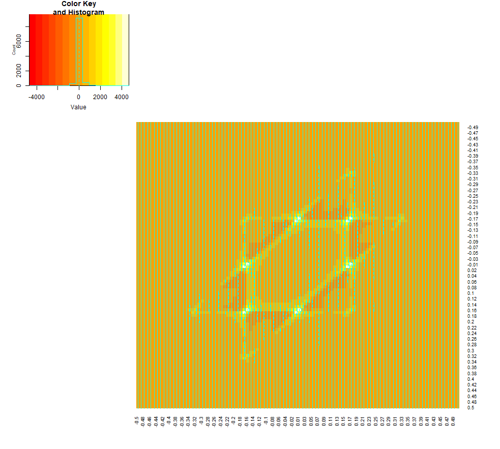
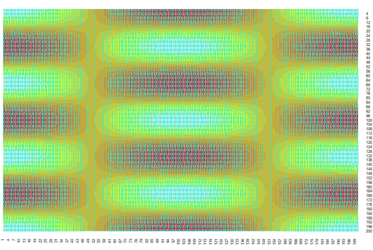
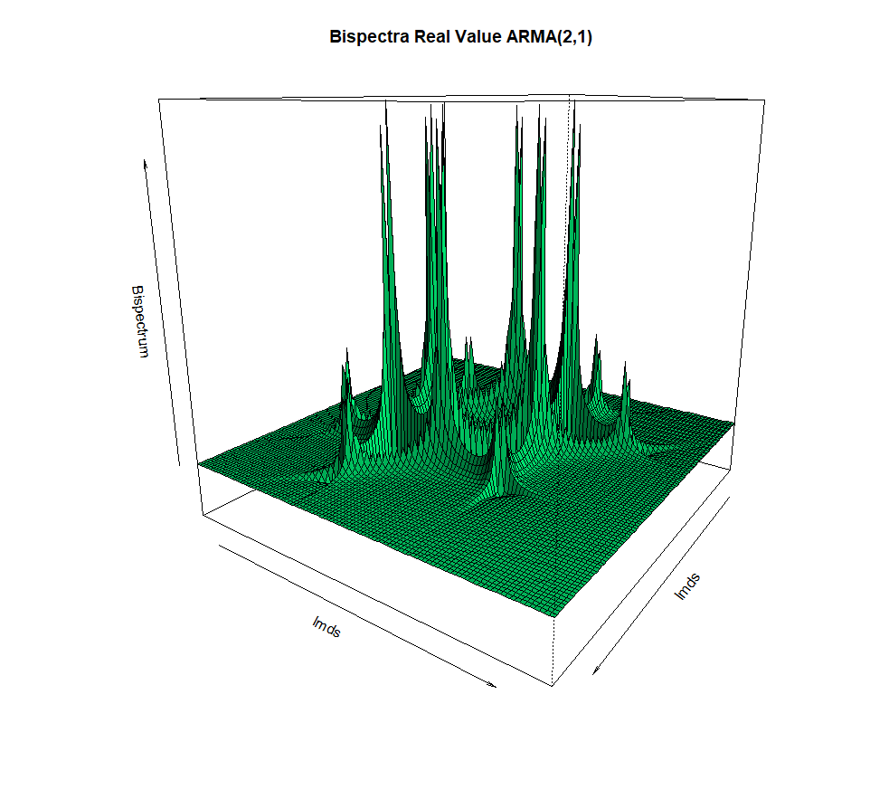
Figure 3: Bispectrum of ARMA(2,1) process with parameters given in Section 5.2, left panel exhibiting the 3d-plot and the right panel showing the heatmap.

Next, we consider an ARMA(2,1) process {Xt}subscript𝑋𝑡\{X_{t}\}, defined via XtXt1+0.9Xt2=ϵt+0.8ϵt1subscript𝑋𝑡subscript𝑋𝑡10.9subscript𝑋𝑡2subscriptitalic-ϵ𝑡0.8subscriptitalic-ϵ𝑡1X_{t}-X_{t-1}+0.9X_{t-2}=\epsilon_{t}+0.8\epsilon_{t-1}, where ϵtExp(1)1similar-tosubscriptitalic-ϵ𝑡Exp11\epsilon_{t}\sim\mbox{Exp}(1)-1, i.e. ϕ(z)=1z+0.9z2italic-ϕ𝑧1𝑧0.9superscript𝑧2\phi(z)=1-z+0.9z^{2} and θ(z)=1+0.8z𝜃𝑧10.8𝑧\theta(z)=1+0.8z, where ϕ(B)Xt=θ(B)ϵtitalic-ϕ𝐵subscript𝑋𝑡𝜃𝐵subscriptitalic-ϵ𝑡\phi(B)X_{t}=\theta(B)\epsilon_{t}. Hence, Ψ(z)=θ(z)/ϕ(z)=(1+0.8z)/(1z+0.9z2)Ψ𝑧𝜃𝑧italic-ϕ𝑧10.8𝑧1𝑧0.9superscript𝑧2\Psi(z)=\theta(z)/\phi(z)=(1+0.8z)/(1-z+0.9z^{2}). The spectra, bispectra, and trispectra are:

f(λ)=|Ψ(eιλ)|2,f(λ,ω)=2Ψ(eιλ)Ψ(eιω)Ψ(eι(λ+ω)),andformulae-sequence𝑓𝜆superscriptΨsuperscript𝑒𝜄𝜆2𝑓𝜆𝜔2Ψsuperscript𝑒𝜄𝜆Ψsuperscript𝑒𝜄𝜔Ψsuperscript𝑒𝜄𝜆𝜔and\displaystyle f(\lambda)=\lvert\Psi(e^{-\iota\lambda})\rvert^{2},\quad f(\lambda,\omega)=2\Psi(e^{-\iota\lambda})\Psi(e^{-\iota\omega})\Psi(e^{\iota(\lambda+\omega)}),~{}~{}\mbox{and}
f(λ1,λ2,λ3)=9Ψ(eιλ1)Ψ(eιλ2)Ψ(eιλ3)Ψ(eι(λ1+λ2+λ3)).𝑓subscript𝜆1subscript𝜆2subscript𝜆39Ψsuperscript𝑒𝜄subscript𝜆1Ψsuperscript𝑒𝜄subscript𝜆2Ψsuperscript𝑒𝜄subscript𝜆3Ψsuperscript𝑒𝜄subscript𝜆1subscript𝜆2subscript𝜆3\displaystyle f(\lambda_{1},\lambda_{2},\lambda_{3})=9\Psi(e^{-\iota\lambda_{1}})\Psi(e^{-\iota\lambda_{2}})\Psi(e^{-\iota\lambda_{3}})\Psi(e^{\iota(\lambda_{1}+\lambda_{2}+\lambda_{3})}).

The bispectra of the ARMA(2,1) process is depicted in Figure 3. We also consider this process with ϵtχ424similar-tosubscriptitalic-ϵ𝑡subscriptsuperscript𝜒244\epsilon_{t}\sim\chi^{2}_{4}-4, which changes the scale of the polyspectra.

5.3 Squared Hermite

The final example is a squared Hermite process defined by Xt=J1H1(Zt)+J2H2(Zt)=J1Zt+J2Zt2J2subscript𝑋𝑡subscript𝐽1subscript𝐻1subscript𝑍𝑡subscript𝐽2subscript𝐻2subscript𝑍𝑡subscript𝐽1subscript𝑍𝑡subscript𝐽2superscriptsubscript𝑍𝑡2subscript𝐽2X_{t}=J_{1}\,H_{1}(Z_{t})+J_{2}\,H_{2}(Z_{t})=J_{1}\,Z_{t}+J_{2}\,Z_{t}^{2}-J_{2}, where J1=2subscript𝐽12J_{1}=2, J2=5subscript𝐽25J_{2}=5, and {Zt}subscript𝑍𝑡\{Z_{t}\} is a MA(1) process such that Zt=ϵt+0.4ϵt1subscript𝑍𝑡subscriptitalic-ϵ𝑡0.4subscriptitalic-ϵ𝑡1Z_{t}=\epsilon_{t}+0.4\epsilon_{t-1} with ϵtExp(1)1similar-tosubscriptitalic-ϵ𝑡Exp11\epsilon_{t}\sim\mbox{Exp}(1)-1. The autocumulants are

γ(h1)𝛾subscript1\displaystyle\gamma(h_{1}) =J12c(h1)+J22c(h1)2absentsuperscriptsubscript𝐽12𝑐subscript1superscriptsubscript𝐽22𝑐superscriptsubscript12\displaystyle=J_{1}^{2}\,c(h_{1})+J_{2}^{2}\,{c(h_{1})}^{2}
γ3(h1,h2)subscript𝛾3subscript1subscript2\displaystyle\gamma_{3}(h_{1},h_{2}) =2J12J2(c(h1)c(h2)+c(h1)c(h1h2)+c(h2)c(h1h2))absent2superscriptsubscript𝐽12subscript𝐽2𝑐subscript1𝑐subscript2𝑐subscript1𝑐subscript1subscript2𝑐subscript2𝑐subscript1subscript2\displaystyle=\sqrt{2}J_{1}^{2}J_{2}\,\left(c(h_{1})c(h_{2})+c(h_{1})c(h_{1}-h_{2})+c(h_{2})c(h_{1}-h_{2})\right)
+(2J2)3c(h1)c(h2)c(h1h2).superscript2subscript𝐽23𝑐subscript1𝑐subscript2𝑐subscript1subscript2\displaystyle+{(\sqrt{2}J_{2})}^{3}\,c(h_{1})\,c(h_{2})\,c(h_{1}-h_{2}).

The expression for γ4(h1,h2,h3)subscript𝛾4subscript1subscript2subscript3\gamma_{4}(h_{1},h_{2},h_{3}) is very long, and is given in the Supplement Ghosh et al. [2024].

5.4 Simulation Results

For each of these three processes, we construct bispectral means from the following weight functions:

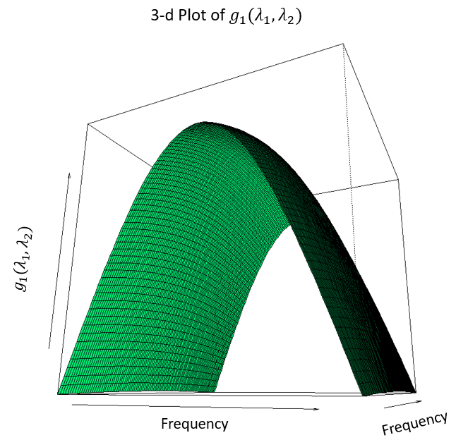
  • g1(λ1,λ2)=(4π)2cos(3λ1)cos(λ2)subscript𝑔1subscript𝜆1subscript𝜆2superscript4𝜋2𝑐𝑜𝑠3subscript𝜆1𝑐𝑜𝑠subscript𝜆2g_{1}(\lambda_{1},\lambda_{2})=(4\pi)^{-2}cos(3\lambda_{1})cos(\lambda_{2}) (as discussed in Example 1)

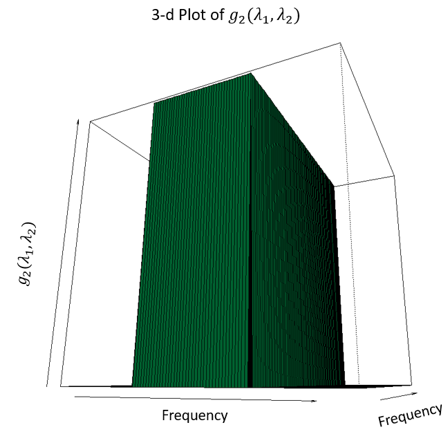
  • g2(λ1,λ2)=𝕀[0.2,0.2](λ1)𝕀[0.5,0.5](λ2)subscript𝑔2subscript𝜆1subscript𝜆2subscript𝕀0.20.2subscript𝜆1subscript𝕀0.50.5subscript𝜆2g_{2}(\lambda_{1},\lambda_{2})=\mathbb{I}_{[-0.2,0.2]}(\lambda_{1})\mathbb{I}_{[-0.5,0.5]}(\lambda_{2}) (as discussed in Example 4)

  • g(λ1,λ2)=1λ12+λ222𝑔subscript𝜆1subscript𝜆21superscriptsubscript𝜆12superscriptsubscript𝜆222g(\lambda_{1},\lambda_{2})=1-\sqrt{\frac{\lambda_{1}^{2}+\lambda_{2}^{2}}{2}}

Refer to caption
Refer to caption
Refer to caption
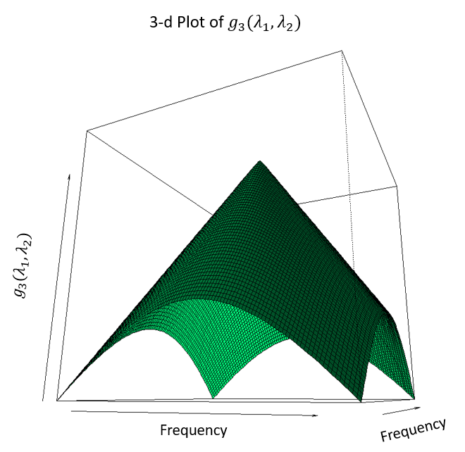
Figure 4: 3-d plot of the weight functions given in the text. Polyspectral means with different weight functions provide different features of the time series.

The 3-d plots of the weight functions are given in Figure 4. Each choice of g𝑔g determines the parameter Mg(f2)subscript𝑀𝑔subscript𝑓2M_{g}(f_{2}), and we also compute the true asymptotic variance V𝑉V as given in (3.7). Next, we compute Mg(f2)^^subscript𝑀𝑔subscript𝑓2\widehat{M_{g}(f_{2})} from simulations of length T=100𝑇100T=100, with 100010001000 replications. The sample variance of these 100010001000 values of Mg(f2)^^subscript𝑀𝑔subscript𝑓2\widehat{M_{g}(f_{2})} provides an estimate V^^𝑉\widehat{V} of V𝑉V; repeating the entire procedure another 100010001000 times yields variance estimates V^isubscript^𝑉𝑖\hat{V}_{i} for 1i10001𝑖10001\leq i\leq 1000. The Mean Squared Error (MSE) and scaled MSE is then computed using the formulas i=11000(V^iV)2superscriptsubscript𝑖11000superscriptsubscript^𝑉𝑖𝑉2\sum_{i=1}^{1000}\left(\hat{V}_{i}-V\right)^{2} and i=11000(V^i/V1)2superscriptsubscript𝑖11000superscriptsubscript^𝑉𝑖𝑉12\sum_{i=1}^{1000}\left(\hat{V}_{i}/V-1\right)^{2}, respectively. The results of the simulation are given in Table 1: for all cases, all models, and all weight functions, the computed asymptotic variance is close in terms of MSE to the simulated quantities.

Table 1: Mean Squared Error (MSE) and scaled MSE of asymptotic variance of polyspectral mean for different processes and different weight functions (Sample Size is 100100100).
Model g(λ¯¯𝜆\underline{\lambda}) MSE Scaled MSE
Model 1: AR(2) with Exp(1)1Exp11\mbox{Exp}(1)-1 errors g1(λ1,λ2)subscript𝑔1subscript𝜆1subscript𝜆2g_{1}(\lambda_{1},\lambda_{2}) 0.003 0.12
g2(λ1,λ2)subscript𝑔2subscript𝜆1subscript𝜆2g_{2}(\lambda_{1},\lambda_{2}) 0.023 0.19
g3(λ1,λ2)subscript𝑔3subscript𝜆1subscript𝜆2g_{3}(\lambda_{1},\lambda_{2}) 0.017 0.26
Model 2: AR(2) with χ424subscriptsuperscript𝜒244\chi^{2}_{4}-4 errors g1(λ1,λ2)subscript𝑔1subscript𝜆1subscript𝜆2g_{1}(\lambda_{1},\lambda_{2}) << 0.005 0.07
g2(λ1,λ2)subscript𝑔2subscript𝜆1subscript𝜆2g_{2}(\lambda_{1},\lambda_{2}) 0.011 0.15
g3(λ1,λ2)subscript𝑔3subscript𝜆1subscript𝜆2g_{3}(\lambda_{1},\lambda_{2}) 0.073 0.82
Model 3: ARMA(2,1) with Exp(1)1Exp11\mbox{Exp}(1)-1 errors g1(λ1,λ2)subscript𝑔1subscript𝜆1subscript𝜆2g_{1}(\lambda_{1},\lambda_{2}) 0.023 0.39
g2(λ1,λ2)subscript𝑔2subscript𝜆1subscript𝜆2g_{2}(\lambda_{1},\lambda_{2}) 0.010 0.40
g3(λ1,λ2)subscript𝑔3subscript𝜆1subscript𝜆2g_{3}(\lambda_{1},\lambda_{2}) 0.027 0.14
Model 4: ARMA(2,1) with χ424subscriptsuperscript𝜒244\chi^{2}_{4}-4 errors g1(λ1,λ2)subscript𝑔1subscript𝜆1subscript𝜆2g_{1}(\lambda_{1},\lambda_{2}) 0.034 0.15
g2(λ1,λ2)subscript𝑔2subscript𝜆1subscript𝜆2g_{2}(\lambda_{1},\lambda_{2}) << 0.005 0.28
g3(λ1,λ2)subscript𝑔3subscript𝜆1subscript𝜆2g_{3}(\lambda_{1},\lambda_{2}) 0.009 1.07
Model 5: Squared Hermite process g1(λ1,λ2)subscript𝑔1subscript𝜆1subscript𝜆2g_{1}(\lambda_{1},\lambda_{2}) 0.081 0.27
g2(λ1,λ2)subscript𝑔2subscript𝜆1subscript𝜆2g_{2}(\lambda_{1},\lambda_{2}) 0.037 0.14
g3(λ1,λ2)subscript𝑔3subscript𝜆1subscript𝜆2g_{3}(\lambda_{1},\lambda_{2}) 0.002 0.91

5.5 Power Curve for Linearity Test

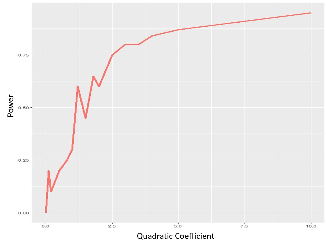
We studied through simulations the power of our proposed linearity test (4.3) with M=10𝑀10M=10, generating the {Xt}subscript𝑋𝑡\{X_{t}\} process from

Xt=ϵt+0.4ϵt1+θϵt12θ,ϵt𝒩(0,1).formulae-sequencesubscript𝑋𝑡subscriptitalic-ϵ𝑡0.4subscriptitalic-ϵ𝑡1𝜃superscriptsubscriptitalic-ϵ𝑡12𝜃similar-tosubscriptitalic-ϵ𝑡𝒩01X_{t}=\epsilon_{t}+0.4\epsilon_{t-1}+\theta\epsilon_{t-1}^{2}-\theta,\quad\epsilon_{t}\sim\mathcal{N}(0,1). (5.5)

Note that when θ=0𝜃0\theta=0 this process is linear, and hence corresponds to the null hypothesis (4.1) of our linearity test statistic. Non-zero values of θ𝜃\theta generate nonlinear effects, corresponding to the alternative hypothesis, and so we can determine power as a function of θ𝜃\theta. We generated 100010001000 simulations of sample size 100100100 of the process (5.5), letting θ𝜃\theta range from 00 to 101010. The power curve (Figure 5) increases with θ𝜃\theta, as anticipated; there are a few jags that are attributed to Monte Carlo error.
Refer to caption
Figure 5: Power Curve of nonlinearity test for different choices of θ𝜃\theta in the process (5.5). Power is increasing in θ𝜃\theta, which parameterizes deviation from linearity.

6 Real Data Analysis

6.1 Sunspot Data Linearity Test

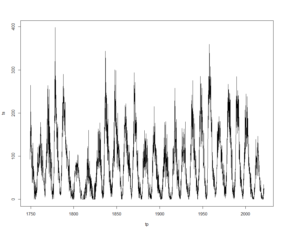
Sunspots are temporary phenomena on the Sun’s photosphere that appear as spots relatively darker than surrounding areas. Those spots are regions of reduced surface temperature arising due to concentrations of magnetic field flux that inhibit convection. It is already known that the solar activity follows a periodic pattern repeating every 11 years Schwabe [1844]. Figure 6 shows the time series of the sunspot data in a monthly interval SILSO World Data Center [1749-2021].
Refer to caption
Figure 6: Time Series of Sunspot Data in a Monthly Interval (Source: SILSO World Data Center [1749-2021]).

McElroy et al. [2023] demonstrated that it is possible to gain significant improvement in prediction in sunspot data by using quadratic prediction instead of linear prediction. This means that there must be nonlinearity present in the sunspot data. Here we will use the test statistic proposed in Section 4 to examine whether the sunspot data follows the particular linear process studied in Abdel-Rahman, Marzouk [2018], namely the order one autoregressive process given by Xt=0.976Xt1+ϵtsubscript𝑋𝑡0.976subscript𝑋𝑡1subscriptitalic-ϵ𝑡X_{t}=0.976X_{t-1}+\epsilon_{t}. In the context of Section 4, this means that ψ(z)=(1.976z)1𝜓𝑧superscript1.976𝑧1\psi(z)={(1-.976z)}^{-1} and Ψ(λ,ω)=(1.976eiλ)1(1.976eiω)1(1.976ei(λ+ω))1Ψ𝜆𝜔superscript1.976superscript𝑒𝑖𝜆1superscript1.976superscript𝑒𝑖𝜔1superscript1.976superscript𝑒𝑖𝜆𝜔1\Psi(\lambda,\omega)={(1-.976e^{-i\lambda})}^{-1}{(1-.976e^{-i\omega})}^{-1}{(1-.976e^{i(\lambda+\omega)})}^{-1}. Choosing M=10𝑀10M=10, the test statistic (4.3) is 𝒯BLT=3740.057subscript𝒯𝐵𝐿𝑇3740.057\mathcal{T}_{BLT}=3740.057, which has a p-value <0.005absent0.005<0.005 (Choosing M=8𝑀8M=8, the test statistic was 𝒯BLT=1945.213subscript𝒯𝐵𝐿𝑇1945.213\mathcal{T}_{BLT}=1945.213 (p-value: <0.005absent0.005<0.005) and choosing M=5𝑀5M=5, we get 𝒯BLT=1312.310subscript𝒯𝐵𝐿𝑇1312.310\mathcal{T}_{BLT}=1312.310 (p-value: <0.005absent0.005<0.005)). Hence, our proposed test rejects the null hypothesis of linearity of the sunspot data, as assumed by Abdel-Rahman, Marzouk [2018].

6.2 GDP Trend Clustering

Time series clustering is a possible application of polyspectral means; by choosing various weighting functions, we can extract different types of information from a time series. In this section, we have analyzed the Gross Domestic Product (GDP) of 136 countries (measured over the past 40 years), and have attempted to classify the growth trend of the GDP of different countries based on the bispectral means taken with different weight functions. The right panel of Figure 1 shows that there are different trend patterns for the various countries, and these diverse patterns are reflected in the differenced time series (left panel of Figure 1); the differencing ensures that the resulting growth rates are stationary. We investigate clustering of these time series through examining bispectral means of their growth rates. The weight functions considered are:

  • g(λ1,λ2)=𝕀(a<λ12+λ22<b)𝑔subscript𝜆1subscript𝜆2𝕀𝑎superscriptsubscript𝜆12superscriptsubscript𝜆22𝑏g(\lambda_{1},\lambda_{2})=\mathbb{I}(a<\lambda_{1}^{2}+\lambda_{2}^{2}<b), where a and b are taken such that the interval (0,1)01(0,1) is split into 10 segments. Hence, we have 10 such bispectral means for each annulus (as discussed in Example 4).

  • g(λ1,λ2)=(π|λ1|)(π|λ2|)𝑔subscript𝜆1subscript𝜆2𝜋subscript𝜆1𝜋subscript𝜆2g(\lambda_{1},\lambda_{2})=(\pi-\lvert\lambda_{1}\rvert)(\pi-\lvert\lambda_{2}\rvert) (as discussed in Example 5).

  • g(λ1,λ2)=(2π)2cos(3λ1)cos(λ2)𝑔subscript𝜆1subscript𝜆2superscript2𝜋2𝑐𝑜𝑠3subscript𝜆1𝑐𝑜𝑠subscript𝜆2g(\lambda_{1},\lambda_{2})=(2\pi)^{-2}cos(3\lambda_{1})cos(\lambda_{2}) (as discussed in Example 1).

Refer to caption
Figure 7: Clustering of 136 countries according to 12 polyspectral means estimated from annual GDP growth rates.

The 12 computed bispectral means are then used to classify the 136 countries into 5 classes, as shown in Figure 7, using k-means clustering. The features considered are all the bispectral means obtained using the given weight functions. The developed EU countries all fall into the same category. The South Asian and South-East countries form another category, while all types of categories are found in Africa and South America. Some developed countries, like the USA and Canada, are members of the same category as undeveloped countries such as Benin, and this is likely due to similar patterns of GDP growth. In other words, the classification algorithm classifies countries based on the growth trend of the GDP rather than the actual GDP, and the fact that USA and Benin are in the same group might be due to the fact that both countries have recently shown similar growth trend in GDP, the reasons behind which might be of practical interest, and can be explored in further studies.

7 Proofs

7.1 Proof of Proposition 3.6

Proof 7.10.

By direct calculation, the expected value of Mg(fk)^)\widehat{M_{g}(f_{k})}) is

E(Mg(fk)^))=(2π)kTk1λ¯~E(d(λ1~)d(λk~,)d([λ¯~]))g(λ¯~).E\left(\widehat{M_{g}(f_{k})})\right)=(2\pi)^{k}T^{-k-1}\sum_{\tilde{\underline{\lambda}}}E\left(d\left(\tilde{\lambda_{1}}\right)\ldots d\left(\tilde{\lambda_{k}},\right)d\left(-[\tilde{\underline{\lambda}}]\right)\right)g\left(\tilde{\underline{\lambda}}\right).

Now, using results from Brillinger, Rosenblatt [1967] we obtain

E(d(λ1~)d(λk~)d([λ¯~]))=στnbσCb.𝐸𝑑~subscript𝜆1𝑑~subscript𝜆𝑘𝑑delimited-[]~¯𝜆subscript𝜎subscript𝜏𝑛subscriptproduct𝑏𝜎subscript𝐶𝑏E\left(d\left(\tilde{\lambda_{1}}\right)\ldots d\left(\tilde{\lambda_{k}}\right)d\left(-[\tilde{\underline{\lambda}}]\right)\right)=\sum_{\sigma\in\tau_{n}}\prod_{b\in\sigma}C_{b}.

The term Cbsubscript𝐶𝑏C_{b} will be non-zero only when the sum of the Fourier frequencies inside the partition is 00, which can only occur when the partition contains all the λ~~𝜆\tilde{\lambda}’s, since the Fourier Frequencies are assumed not to lie in any sub-manifold. Therefore, E(d(λ1~)d(λk~)d([λ¯~]))=Cum(d(λ1~),,d(λk~),d([λ¯~]))=Tf(λ¯~)+O(1),𝐸𝑑~subscript𝜆1𝑑~subscript𝜆𝑘𝑑delimited-[]~¯𝜆Cum𝑑~subscript𝜆1𝑑~subscript𝜆𝑘𝑑delimited-[]~¯𝜆𝑇𝑓~¯𝜆𝑂1E\left(d\left(\tilde{\lambda_{1}}\right)\ldots d\left(\tilde{\lambda_{k}}\right)d\left(-[\tilde{\underline{\lambda}}]\right)\right)=\mbox{Cum}\left(d\left(\tilde{\lambda_{1}}\right),\ldots,d\left(\tilde{\lambda_{k}}\right),d\left(-[\tilde{\underline{\lambda}}]\right)\right)=Tf\left(\tilde{\underline{\lambda}}\right)+O(1), where the last equality is a direct outcome of Lemma 1 of Brillinger, Rosenblatt [1967], and the error term is uniform for all {λ1~,,λk~}~subscript𝜆1~subscript𝜆𝑘\{\tilde{\lambda_{1}},\ldots,\tilde{\lambda_{k}}\}. Hence, using the convergence of a Riemann sum to an integral form (which is valid given the properties of the weight function), we obtain EMg(f)^=(2π)kTk1λ¯~[Tf(λ¯~)+O(1)]g(λ¯~)=Mg(f)+o(1)𝐸^subscript𝑀𝑔𝑓superscript2𝜋𝑘superscript𝑇𝑘1subscript~¯𝜆delimited-[]𝑇𝑓~¯𝜆𝑂1𝑔~¯𝜆subscript𝑀𝑔𝑓𝑜1E\widehat{M_{g}(f)}=(2\pi)^{k}T^{-k-1}\sum_{\tilde{\underline{\lambda}}}\big{[}Tf(\tilde{\underline{\lambda}})+O(1)\big{]}g(\tilde{\underline{\lambda}})=M_{g}\left(f\right)+o(1). Note that by (3.1), the k𝑘kth order polyspectrum is bounded. Hence, it is easy to show that the o(1)𝑜1o(1)-term is indeed O(T1)𝑂superscript𝑇1O\left(T^{-1}\right) when (3.3) holds.

7.2 Proof of Proposition 2

Proof 7.11.

Recall that (3.4) has been established, and hence from (3.4) and (3.5) we only need to examine σI2k+2bσCbsubscript𝜎subscript𝐼2𝑘2subscriptproduct𝑏𝜎subscript𝐶𝑏\sum_{\sigma\in I_{2k+2}}\prod_{b\in\sigma}C_{b}. From Lemma 1 of Brillinger, Rosenblatt [1967], under the assumption that |vjca1,,ak(v1,,vk1)|<subscript𝑣𝑗subscriptsuperscript𝑐subscript𝑎1subscript𝑎𝑘subscript𝑣1subscript𝑣𝑘1\sum\lvert v_{j}c^{\prime}_{a_{1},\ldots,a_{k}}(v_{1},\ldots,v_{k-1})\rvert<\infty, this term is non-zero if and only if the sum of the frequencies is 0. Recall that {λ¯}¯𝜆\{\underline{\lambda}\} is a shorthand for {λ1,,λk,[λ¯]}subscript𝜆1subscript𝜆𝑘delimited-[]¯𝜆\{\lambda_{1},\ldots,\lambda_{k},-[\underline{\lambda}]\}. Then it follows that the terms bσCbsubscriptproduct𝑏𝜎subscript𝐶𝑏\prod_{b\in\sigma}C_{b} will be non-zero in two possible partitioning of the vector {{λ¯},{ω¯}}¯𝜆¯𝜔\{\{\underline{\lambda}\},-\{\underline{\omega}\}\}, as given in Section 3. As we described in the referred section, there are two possible partitions, one with two sets containing elements only from {λ¯}¯𝜆\{\underline{\lambda}\} and {ω¯}¯𝜔-\{\underline{\omega}\}, and others with a mixture of each vector, such that every set contains at least one element from each vector.

In the first case, we have only one partition with two sets, namely, {{λ¯},{ω¯}}¯𝜆¯𝜔\{\{\underline{\lambda}\},-\{\underline{\omega}\}\}. Let us denote this partition by σ0subscript𝜎0\sigma_{0}. Since the sum of elements of both partitions is zero, both of them will contribute non-zero values to the product, rendering the product to be non-zero. Hence bσ0Cbsubscriptproduct𝑏subscript𝜎0subscript𝐶𝑏\prod_{b\in\sigma_{0}}C_{b} can be written as

=Cum(d(λ1),,d(λk),d([λ¯]))Cum(d(ω1),,d(ωk),d([ω¯]))absentCum𝑑subscript𝜆1𝑑subscript𝜆𝑘𝑑delimited-[]¯𝜆Cum𝑑subscript𝜔1𝑑subscript𝜔𝑘𝑑delimited-[]¯𝜔\displaystyle=\mbox{Cum}\left(d(\lambda_{1}),\ldots,d(\lambda_{k}),d\left(-[\underline{\lambda}]\right)\right)\mbox{Cum}\left(d(-\omega_{1}),\ldots,d(-\omega_{k}),d\left([\underline{\omega}]\right)\right)
=(Tf(λ¯)+O(1))(Tf(ω¯)+O(1))absent𝑇𝑓¯𝜆𝑂1𝑇𝑓¯𝜔𝑂1\displaystyle=\left(Tf(\underline{\lambda})+O(1)\right)\left(Tf(-\underline{\omega})+O(1)\right)
=T2f(λ¯)f(ω¯)+O(T).absentsuperscript𝑇2𝑓¯𝜆𝑓¯𝜔𝑂𝑇\displaystyle=T^{2}f(\underline{\lambda})f(-\underline{\omega})+O(T).

Hence, substituting the value of bσ0Cbsubscriptproduct𝑏subscript𝜎0subscript𝐶𝑏\prod_{b\in\sigma_{0}}C_{b} in the sum of (3.5), we obtain the following:

T2k2(2π)2kλ¯~,ω¯~g(λ¯~)g(ω¯~)¯{T2f(λ¯~)f(ω¯~)+O(T)}superscript𝑇2𝑘2superscript2𝜋2𝑘subscript~¯𝜆~¯𝜔𝑔~¯𝜆¯𝑔~¯𝜔superscript𝑇2𝑓~¯𝜆𝑓~¯𝜔𝑂𝑇\displaystyle T^{-2k-2}(2\pi)^{2k}\sum_{\tilde{\underline{\lambda}},\tilde{\underline{\omega}}}g(\tilde{\underline{\lambda}})\overline{g(\tilde{\underline{\omega}})}\left\{T^{2}f(\tilde{\underline{\lambda}})f(-\tilde{\underline{\omega}})+O(T)\right\}
=\displaystyle= T2k(2π)2kλ¯~,ω¯~g(λ¯~)g(ω¯~)¯f(λ¯~)f(ω¯~)+(2π)2kT2kλ¯~,ω¯~g(λ¯~)g(ω¯~)¯O(T1).superscript𝑇2𝑘superscript2𝜋2𝑘subscript~¯𝜆~¯𝜔𝑔~¯𝜆¯𝑔~¯𝜔𝑓~¯𝜆𝑓~¯𝜔superscript2𝜋2𝑘superscript𝑇2𝑘subscript~¯𝜆~¯𝜔𝑔~¯𝜆¯𝑔~¯𝜔𝑂superscript𝑇1\displaystyle T^{-2k}\left(2\pi\right)^{2k}\sum_{\tilde{\underline{\lambda}},\tilde{\underline{\omega}}}g(\tilde{\underline{\lambda}})\overline{g(\tilde{\underline{\omega}})}f(\tilde{\underline{\lambda}})f(-\tilde{\underline{\omega}})+(2\pi)^{2k}T^{-2k}\sum_{\tilde{\underline{\lambda}},\tilde{\underline{\omega}}}g(\tilde{\underline{\lambda}})\overline{g(\tilde{\underline{\omega}})}\cdot O\left(T^{-1}\right).

Thus, the final expression is Mg(f)Mg(f)¯+O(T1)subscript𝑀𝑔𝑓¯subscript𝑀𝑔𝑓𝑂superscript𝑇1M_{g}(f)\overline{M_{g}(f)}+O(T^{-1}), which in view of (3.4) leaves a O(T1)𝑂superscript𝑇1O(T^{-1}) term. The terms O(T)𝑂𝑇O(T) and O(T1)𝑂superscript𝑇1O\left(T^{-1}\right) are uniform in {λ1,,λk}subscript𝜆1subscript𝜆𝑘\{\lambda_{1},\ldots,\lambda_{k}\}, as given in Brillinger, Rosenblatt [1967].

The second case can have multiple possible partitions, where every set of every partition must contain a mixture of {λ¯}¯𝜆\{\underline{\lambda}\} and {ω¯}¯𝜔-\{\underline{\omega}\}. Let us first consider the special case where we have only one set in the partition, i.e. the partition consists only of {{λ¯},{ω¯}}¯𝜆¯𝜔\{\{\underline{\lambda}\},-\{\underline{\omega}\}\}. Let us call this partition as σ1subscript𝜎1\sigma_{1}. Then,

bσ1Cbsubscriptproduct𝑏subscript𝜎1subscript𝐶𝑏\displaystyle\prod_{b\in\sigma_{1}}C_{b} =Cum(d(λ1),,d(λk),d([λ¯]),d(ω1),,d(ωk),d([ω¯]))absentCum𝑑subscript𝜆1𝑑subscript𝜆𝑘𝑑delimited-[]¯𝜆𝑑subscript𝜔1𝑑subscript𝜔𝑘𝑑delimited-[]¯𝜔\displaystyle=\mbox{Cum}\left(d(\lambda_{1}),\ldots,d(\lambda_{k}),d\left(-[\underline{\lambda}]\right),d(-\omega_{1}),\ldots,d(-\omega_{k}),d\left([\underline{\omega}]\right)\right)
=Tf2k+1(λ¯,[λ¯],ω¯)+O(1).absent𝑇subscript𝑓2𝑘1¯𝜆delimited-[]¯𝜆¯𝜔𝑂1\displaystyle=Tf_{2k+1}(\underline{\lambda},-[\underline{\lambda}],-\underline{\omega})+O(1).

Hence, again substituting the value of bσ1Cbsubscriptproduct𝑏subscript𝜎1subscript𝐶𝑏\prod_{b\in\sigma_{1}}C_{b} in the sum (3.5) we obtain

T2k2(2π)2kλ¯~,ω¯~g(λ¯~)g(ω¯~)¯{Tf2k+1(λ¯~,[λ¯~],ω¯~)+O(1)}superscript𝑇2𝑘2superscript2𝜋2𝑘subscript~¯𝜆~¯𝜔𝑔~¯𝜆¯𝑔~¯𝜔𝑇subscript𝑓2𝑘1~¯𝜆delimited-[]~¯𝜆~¯𝜔𝑂1\displaystyle T^{-2k-2}(2\pi)^{2k}\sum_{\tilde{\underline{\lambda}},\tilde{\underline{\omega}}}g(\tilde{\underline{\lambda}})\overline{g(\tilde{\underline{\omega}})}\left\{Tf_{2k+1}(\tilde{\underline{\lambda}},-[\tilde{\underline{\lambda}}],-\tilde{\underline{\omega}})+O(1)\right\}
=T2k1(2π)2kλ¯~,ω¯~g(λ¯~)g(ω¯~)¯f2k+1(λ¯~,[λ¯~],ω¯~)+(2π)2kT2kλ¯~,ω¯~g(λ¯~,ω¯~)O(T2)absentsuperscript𝑇2𝑘1superscript2𝜋2𝑘subscript~¯𝜆~¯𝜔𝑔~¯𝜆¯𝑔~¯𝜔subscript𝑓2𝑘1~¯𝜆delimited-[]~¯𝜆~¯𝜔superscript2𝜋2𝑘superscript𝑇2𝑘subscript~¯𝜆~¯𝜔𝑔~¯𝜆~¯𝜔𝑂superscript𝑇2\displaystyle=T^{-2k-1}(2\pi)^{2k}\sum_{\tilde{\underline{\lambda}},\tilde{\underline{\omega}}}g(\tilde{\underline{\lambda}})\overline{g(\tilde{\underline{\omega}})}f_{2k+1}(\tilde{\underline{\lambda}},-[\tilde{\underline{\lambda}}],-\tilde{\underline{\omega}})+(2\pi)^{2k}T^{-2k}\sum_{\tilde{\underline{\lambda}},\tilde{\underline{\omega}}}g(\tilde{\underline{\lambda}},\tilde{\underline{\omega}})\cdot O\left(T^{-2}\right)
=[T1ππππg(λ¯)g(ω¯)¯f2k+1(λ¯,[λ¯],ω¯)𝑑λ¯𝑑ω¯](1+o(1))+O(T2).absentdelimited-[]superscript𝑇1superscriptsubscript𝜋𝜋superscriptsubscript𝜋𝜋𝑔¯𝜆¯𝑔¯𝜔subscript𝑓2𝑘1¯𝜆delimited-[]¯𝜆¯𝜔differential-d¯𝜆differential-d¯𝜔1𝑜1𝑂superscript𝑇2\displaystyle=\Big{[}T^{-1}\int_{-\pi}^{\pi}\ldots\int_{-\pi}^{\pi}g(\underline{\lambda})\overline{g(\underline{\omega})}f_{2k+1}(\underline{\lambda},-[\underline{\lambda}],-\underline{\omega})d\underline{\lambda}d\underline{\omega}\Big{]}\big{(}1+o(1)\big{)}+O(T^{-2}).

Hence, the final expression will be a polyspectral mean of order 2k+12𝑘12k+1, with a weight function depending on the original weight function.

The third case includes the situation where if the blocks of a partition σ𝜎\sigma are b1,b2,,bpsubscript𝑏1subscript𝑏2subscript𝑏𝑝b_{1},b_{2},\ldots,b_{p}, and the bisubscript𝑏𝑖b_{i} block contains elements λbi1,,λbil,ωbi1,,ωbimsubscript𝜆subscript𝑏𝑖1subscript𝜆subscript𝑏𝑖𝑙subscript𝜔subscript𝑏𝑖1subscript𝜔subscript𝑏𝑖𝑚\lambda_{b_{i1}},\ldots,\lambda_{b_{il}},-\omega_{b_{i1}},\ldots,-\omega_{b_{im}}, then the sums of all those elements must be 00 for each of the blocks bisubscript𝑏𝑖b_{i}. This is because if any of the blocks has elements which do not add up to 00, the corresponding Cbsubscript𝐶𝑏C_{b} will be zero, and hence bσCbsubscriptproduct𝑏𝜎subscript𝐶𝑏\prod_{b\in\sigma}C_{b} will become zero for that partition. Now, we have ensured that no subset of the Fourier frequencies lies in a sub-manifold, i.e., for no subset of λ1,,λksubscript𝜆1subscript𝜆𝑘\lambda_{1},\ldots,\lambda_{k} can the sum be 00. Hence, for one partition to have a non-zero value, all of its blocks must contain at least one element from each of λ𝜆\lambda and ω𝜔\omega. The only other case is covered in the first case, where the partition contains all elements of λ𝜆\lambda and ω𝜔\omega. Now that we know that every block of the partition contains a mixture of {λ¯}¯𝜆\{\underline{\lambda}\} and {ω¯}¯𝜔\{\underline{\omega}\}, let us call each mixture a constraint since each mixture should have a sum 0, and hence would produce a constraint and thereby reducing the degrees of freedom by 1. Suppose we have m𝑚m such constraints, i.e., m𝑚m linear combinations of λksubscript𝜆𝑘\lambda_{k} and ωksubscript𝜔𝑘\omega_{k} are 00. This also means we have m𝑚m blocks. Then we will have a Tmsuperscript𝑇𝑚T^{m} factor from the integrand since every block would contribute a T𝑇T from the cumulant, and a O(1)𝑂1O(1) from the residual. The sum will hence run for only the above cases, i.e., only when the linear combinations of the elements of partitions are equal to 0. In other words, only when there exists A,B~m,k+1𝐴𝐵subscript~𝑚𝑘1A,B\in\widetilde{\mathcal{B}}_{m,k+1} such that A{λ¯}=B{ω¯}𝐴¯𝜆𝐵¯𝜔A\{\underline{\lambda}\}=B\{\underline{\omega}\}, where {λ¯}={λ1,,λk,[λ¯]}¯𝜆subscript𝜆1subscript𝜆𝑘delimited-[]¯𝜆\{\underline{\lambda}\}=\{\lambda_{1},\ldots,\lambda_{k},-[\underline{\lambda}]\}. Recall that the rows and columns of A𝐴A (and B𝐵B) have the properties delineated in the definition of ~m,k+1subscript~𝑚𝑘1\widetilde{\mathcal{B}}_{m,k+1}, arising from the properties of the partition.

Let fα(λ¯α)subscript𝑓𝛼subscript¯𝜆𝛼f_{\alpha}(\underline{\lambda}_{\alpha}), rAjsubscript𝑟𝐴𝑗r_{Aj}, rBjsubscript𝑟𝐵𝑗r_{Bj}, rjsubscript𝑟𝑗r_{j}, λrAjsubscript𝜆subscript𝑟subscript𝐴𝑗\lambda_{r_{A_{j}}}, and ωrBjsubscript𝜔subscript𝑟subscript𝐵𝑗\omega_{r_{B_{j}}} be as defined in Section 3. Then each term inside of the sum of (3.5) is given by (recall the notation f~({λ¯})=f(λ¯)~𝑓¯𝜆𝑓¯𝜆\tilde{f}(\{\underline{\lambda}\})=f(\underline{\lambda}) introduced previously)

Tmj=1mf~rj(λrAj,ωrBj)+O(Tm1).superscript𝑇𝑚superscriptsubscriptproduct𝑗1𝑚subscript~𝑓subscript𝑟𝑗subscript𝜆subscript𝑟subscript𝐴𝑗subscript𝜔subscript𝑟subscript𝐵𝑗𝑂superscript𝑇𝑚1T^{m}\prod_{j=1}^{m}\tilde{f}_{r_{j}}\left(\lambda_{r_{A_{j}}},\omega_{r_{B_{j}}}\right)+O\left(T^{m-1}\right).

Now, for each of these quantities, we have m1𝑚1m-1 constraints (m𝑚m of which arise from each row of the matrices in ~m,k+1subscript~𝑚𝑘1\widetilde{\mathcal{B}}_{m,k+1}, lessened by one because of a redundant constraint that the entire sum is 00). Then, for each term we have

T2k2λ¯~,ω¯~g(λ¯~)g(ω¯~)¯{Tmj=1mf~rj(λrAj,ωrBj)+O(Tm1)}superscript𝑇2𝑘2subscript~¯𝜆~¯𝜔𝑔~¯𝜆¯𝑔~¯𝜔superscript𝑇𝑚superscriptsubscriptproduct𝑗1𝑚subscript~𝑓subscript𝑟𝑗subscript𝜆subscript𝑟subscript𝐴𝑗subscript𝜔subscript𝑟subscript𝐵𝑗𝑂superscript𝑇𝑚1\displaystyle T^{-2k-2}\sum_{\tilde{\underline{\lambda}},\tilde{\underline{\omega}}}g\left(\tilde{\underline{\lambda}}\right)\overline{g\left(\tilde{\underline{\omega}}\right)}\left\{T^{m}\prod_{j=1}^{m}\tilde{f}_{r_{j}}\left(\lambda_{r_{A_{j}}},\omega_{r_{B_{j}}}\right)+O\left(T^{m-1}\right)\right\}
=T1T2k+m1λ¯~,ω¯~g(λ¯~)g(ω¯~)¯j=1mf~rj(λrAj,ωrBj)+O(T2).absentsuperscript𝑇1superscript𝑇2𝑘𝑚1subscript~¯𝜆~¯𝜔𝑔~¯𝜆¯𝑔~¯𝜔superscriptsubscriptproduct𝑗1𝑚subscript~𝑓subscript𝑟𝑗subscript𝜆subscript𝑟subscript𝐴𝑗subscript𝜔subscript𝑟subscript𝐵𝑗𝑂superscript𝑇2\displaystyle=T^{-1}T^{-2k+m-1}\sum_{\tilde{\underline{\lambda}},\tilde{\underline{\omega}}}g\left(\tilde{\underline{\lambda}}\right)\overline{g\left(\tilde{\underline{\omega}}\right)}\prod_{j=1}^{m}\tilde{f}_{r_{j}}\left(\lambda_{r_{A_{j}}},\omega_{r_{B_{j}}}\right)+O\left(T^{-2}\right).

This goes to 0 at rate T1superscript𝑇1T^{-1}. Recall the definitions of Lmsubscript𝐿𝑚L_{m}, l¯¯𝑙\underline{l} and ζl¯subscript𝜁¯𝑙\zeta_{\underline{l}} from Section 3. Then we will have the summation in (3.5) running over all possible choices of matrices A𝐴A and B𝐵B within the sets ζl¯subscript𝜁¯𝑙\zeta_{\underline{l}} for all choices of l¯Lm¯𝑙subscript𝐿𝑚\underline{l}\in L_{m}, such that A{λ¯}=B{ω¯}𝐴¯𝜆𝐵¯𝜔A\{\underline{\lambda}\}=B\{\underline{\omega}\}. Then each of the summands will be of the form

T2k2Tmλ¯~,ω¯~|A{λ¯}=B{ω¯}g(λ¯~)g(ω¯~)¯j=1mf~rj(λrAj,ωrBj),superscript𝑇2𝑘2superscript𝑇𝑚subscript~¯𝜆conditional~¯𝜔𝐴¯𝜆𝐵¯𝜔𝑔~¯𝜆¯𝑔~¯𝜔superscriptsubscriptproduct𝑗1𝑚subscript~𝑓subscript𝑟𝑗subscript𝜆subscript𝑟subscript𝐴𝑗subscript𝜔subscript𝑟subscript𝐵𝑗T^{-2k-2}T^{m}\sum_{\tilde{\underline{\lambda}},\tilde{\underline{\omega}}|A\{\underline{\lambda}\}=B\{\underline{\omega}\}}g\left(\tilde{\underline{\lambda}}\right)\overline{g\left(\tilde{\underline{\omega}}\right)}\prod_{j=1}^{m}\tilde{f}_{r_{j}}\left(\lambda_{r_{A_{j}}},\omega_{r_{B_{j}}}\right),

and the powers of T𝑇T can be expressed as T1T2k+m1superscript𝑇1superscript𝑇2𝑘𝑚1T^{-1}T^{-2k+m-1}. It follows that the second cumulant is of the form

T1m=1k+1l¯LmT2k+m1λ¯~,ω¯~|A{λ¯}=B{ω¯}g(λ¯~)g(ω¯~)¯j=1mf~rj(λrAj,ωrBj)+O(T2),superscript𝑇1superscriptsubscript𝑚1𝑘1subscript¯𝑙subscript𝐿𝑚superscript𝑇2𝑘𝑚1subscript~¯𝜆conditional~¯𝜔𝐴¯𝜆𝐵¯𝜔𝑔~¯𝜆¯𝑔~¯𝜔superscriptsubscriptproduct𝑗1𝑚subscript~𝑓subscript𝑟𝑗subscript𝜆subscript𝑟subscript𝐴𝑗subscript𝜔subscript𝑟subscript𝐵𝑗𝑂superscript𝑇2T^{-1}\sum_{m=1}^{k+1}\sum_{\underline{l}\in L_{m}}T^{-2k+m-1}\sum_{\tilde{\underline{\lambda}},\tilde{\underline{\omega}}|A\{\underline{\lambda}\}=B\{\underline{\omega}\}}g\left(\tilde{\underline{\lambda}}\right)\overline{g\left(\tilde{\underline{\omega}}\right)}\prod_{j=1}^{m}\tilde{f}_{r_{j}}\left(\lambda_{r_{A_{j}}},\omega_{r_{B_{j}}}\right)+O(T^{-2}),

from which the stated formula for V𝑉V (3.7) is obtained. The case m=1𝑚1m=1 is the second case mentioned earlier, which would give a polyspectral mean of order 2k+12𝑘12k+1. This completes the proof.

7.3 Proof of Corollary 1

Proof 7.12.

The proof follows from the fact that

Cov(Mg1(fk)^,Mg1(fk)^)¯\displaystyle Cov(\widehat{M_{g_{1}}(f_{k})},\overline{\widehat{M_{g_{1}}(f_{k})})}
=E{Tkλ¯~kf^k(λ¯~k)g1(λ¯~k)Tk1λ¯~k+1f^k+1(λ¯~k+1)g2(λ¯~k+1)¯}Mg1(fk)Mg2(fk+1)absent𝐸superscript𝑇𝑘subscriptsubscript~¯𝜆𝑘subscript^𝑓𝑘subscript~¯𝜆𝑘subscript𝑔1subscript~¯𝜆𝑘superscript𝑇𝑘1subscriptsubscript~¯𝜆𝑘1subscript^𝑓𝑘1subscript~¯𝜆𝑘1¯subscript𝑔2subscript~¯𝜆𝑘1subscript𝑀subscript𝑔1subscript𝑓𝑘subscript𝑀subscript𝑔2subscript𝑓𝑘1\displaystyle=E\left\{T^{-k}\sum_{\tilde{\underline{\lambda}}_{k}}\hat{f}_{k}(\tilde{\underline{\lambda}}_{k})g_{1}(\tilde{\underline{\lambda}}_{k})T^{-k-1}\sum_{\tilde{\underline{\lambda}}_{k+1}}\hat{f}_{k+1}(\tilde{\underline{\lambda}}_{k+1})\overline{g_{2}(\tilde{\underline{\lambda}}_{k+1})}\right\}-M_{g_{1}}(f_{k})M_{g_{2}}(f_{k+1})
=T2k3(2π)2k+1λ¯~k,ω¯~k+1g1(λ¯~k)g2(λ¯~k+1)¯σI2k+3bσCbMg1(fk)Mg2(fk+1).absentsuperscript𝑇2𝑘3superscript2𝜋2𝑘1subscriptsubscript~¯𝜆𝑘subscript~¯𝜔𝑘1subscript𝑔1subscript~¯𝜆𝑘¯subscript𝑔2subscript~¯𝜆𝑘1subscript𝜎subscript𝐼2𝑘3subscriptproduct𝑏𝜎subscript𝐶𝑏subscript𝑀subscript𝑔1subscript𝑓𝑘subscript𝑀subscript𝑔2subscript𝑓𝑘1\displaystyle=T^{-2k-3}(2\pi)^{2k+1}\sum_{\tilde{\underline{\lambda}}_{k},\tilde{\underline{\omega}}_{k+1}}g_{1}(\tilde{\underline{\lambda}}_{k})\overline{g_{2}(\tilde{\underline{\lambda}}_{k+1})}\sum_{\sigma\in I_{2k+3}}\prod_{b\in\sigma}C_{b}-M_{g_{1}}(f_{k})M_{g_{2}}(f_{k+1}).

In this case, the proof would be similar to previous calculations, except the A𝐴A matrix will be of dimension m×(k+1)𝑚𝑘1m\times(k+1) and the B𝐵B matrix will be of dimension m×(k+2)𝑚𝑘2m\times(k+2). The proof can be easily extended to the covariance between polyspectral means of any two orders.

7.4 Proof of Theorem 3.8

Proof 7.13.

Propositions 1 and 2 give the mean and variance of the limiting distribution. The only thing remaining to prove asymptotic normality is to show that the higher-order cumulants of the scaled transformation go to zero as n goes to \infty. Recalling that {λ¯}=(λ1,,λk,[λ¯])¯𝜆subscript𝜆1subscript𝜆𝑘delimited-[]¯𝜆\{\underline{\lambda}\}=(\lambda_{1},\ldots,\lambda_{k},-[\underline{\lambda}]), we can write (letting Cumr𝐶𝑢subscript𝑚𝑟Cum_{r} denote the rthsuperscript𝑟𝑡r^{th} order joint cumulant)

Cumr(Mg(f)^)𝐶𝑢subscript𝑚𝑟^subscript𝑀𝑔𝑓\displaystyle Cum_{r}(\widehat{M_{g}(f)}) =Cumr(Mg(f)^,,Mg(f)^r times)absent𝐶𝑢subscript𝑚𝑟subscript^subscript𝑀𝑔𝑓^subscript𝑀𝑔𝑓r times\displaystyle=Cum_{r}(\underbrace{\widehat{M_{g}(f)},\ldots,\widehat{M_{g}(f)}}_{\textrm{r times}})
=Cum(Tk1λ¯1g(λ¯1~)d{λ1¯~},,Tk1λ¯r~g(λ¯r~)d{λr¯~})absent𝐶𝑢𝑚superscript𝑇𝑘1subscriptsubscript¯𝜆1𝑔~subscript¯𝜆1product𝑑~¯subscript𝜆1superscript𝑇𝑘1subscript~subscript¯𝜆𝑟𝑔~subscript¯𝜆𝑟product𝑑~¯subscript𝜆𝑟\displaystyle=Cum\left(T^{-k-1}\sum_{\underline{\lambda}_{1}}g(\tilde{\underline{\lambda}_{1}})\prod d\{\tilde{\underline{\lambda_{1}}}\},\ldots,T^{-k-1}\sum_{\tilde{\underline{\lambda}_{r}}}g(\tilde{\underline{\lambda}_{r}})\prod d\{\tilde{\underline{\lambda_{r}}}\}\right)
=Trkrλ1¯~λ¯r~g(λ¯1~)g(λ¯r~)Cum(d{λ1¯~},,d{λr¯~}).absentsuperscript𝑇𝑟𝑘𝑟subscript~¯subscript𝜆1subscript~subscript¯𝜆𝑟𝑔~subscript¯𝜆1𝑔~subscript¯𝜆𝑟𝐶𝑢𝑚product𝑑~¯subscript𝜆1product𝑑~¯subscript𝜆𝑟\displaystyle=T^{-rk-r}\sum_{\tilde{\underline{\lambda_{1}}}}\ldots\sum_{\tilde{\underline{\lambda}_{r}}}g(\tilde{\underline{\lambda}_{1}})\ldots g(\tilde{\underline{\lambda}_{r}})\,Cum\left(\prod d\{\tilde{\underline{\lambda_{1}}}\},\ldots,\prod d\{\tilde{\underline{\lambda_{r}}}\}\right).

Applying Theorem 2.3.3 of Brillinger [2001], we find that

Cum(d{λ1¯~}j,,d{λr¯~}j)𝐶𝑢𝑚product𝑑subscript~¯subscript𝜆1𝑗product𝑑subscript~¯subscript𝜆𝑟𝑗\displaystyle Cum\left(\prod d\{\tilde{\underline{\lambda_{1}}}\}_{j},\ldots,\prod d\{\tilde{\underline{\lambda_{r}}}\}_{j}\right) =νCum(d(λij~):ijν1)Cum(d(λij~):ijνp),\displaystyle=\sum_{\nu}Cum\left(d(\tilde{\lambda_{ij}}):ij\in\nu_{1}\right)\ldots Cum\left(d(\tilde{\lambda_{ij}}):ij\in\nu_{p}\right),

where the summation is over all indecomposible partitions ν=ν1νp𝜈subscript𝜈1subscript𝜈𝑝\nu=\nu_{1}\cup\ldots\cup\nu_{p} of the following table:

((1,1)(1,k+1)(r,1)(r,k+1)).matrix111𝑘1missing-subexpressionmissing-subexpressionmissing-subexpression𝑟1𝑟𝑘1\centering\begin{pmatrix}(1,1)&\cdots&(1,k+1)\\ \cdot&&\cdot\\ \cdot&&\cdot\\ \cdot&&\cdot\\ (r,1)&\cdots&(r,k+1)\\ \end{pmatrix}.\@add@centering

From the expression of cumulants, we know that each of those cumulants is non-zero only when the sum of the corresponding Fourier frequencies inside is equal to zero, and can contribute terms of order at most T𝑇T for each of the partitions, i.e., the highest order from each of these elements is Tpsuperscript𝑇𝑝T^{p}. Hence, to obtain the leading term we would need to take the maximum number of such partitions such that the sum of λ𝜆\lambda’s in the partitions is zero. By our definition of Mg(f)^^subscript𝑀𝑔𝑓\widehat{M_{g}(f)}, no subset of the λ¯isubscript¯𝜆𝑖\underline{\lambda}_{i}’s fall in a sub-manifold. Hence, each of these partitions must contain either all distinct {λ¯}s¯𝜆𝑠\{\underline{\lambda}\}s, or a mixture of λ𝜆\lambda’s. However, if they were all distinct then the partition would not be indecomposable. Hence, we are left with only mixture of λ𝜆\lambda’s. Also, an indecomposable partition would mean that we don’t have any single λ¯¯𝜆\underline{\lambda}, i.e. all the partitions must be a mixture of all the λ𝜆\lambda’s. This is encoded by the matrix notation described earlier. Here we just have r𝑟r matrices A1,Arsubscript𝐴1subscript𝐴𝑟A_{1},\ldots A_{r} such that A1λ¯1++Arλ¯r=0p×1subscript𝐴1subscript¯𝜆1subscript𝐴𝑟subscript¯𝜆𝑟subscript0𝑝1A_{1}\underline{\lambda}_{1}+\ldots+A_{r}\underline{\lambda}_{r}=0_{p\times 1}. Hence, p𝑝p partitions would give p𝑝p constraints, thereby giving an order of Tpsuperscript𝑇𝑝T^{p}, and with these come p1𝑝1p-1 constraints. Therefore, the sum would need to be weighted by Trk+p1superscript𝑇𝑟𝑘𝑝1T^{-rk+p-1} in order to be non-negligible asymptotically, and the remainder term would be Tr+1superscript𝑇𝑟1T^{-r+1}. Thus, the cumulants of order higher than r𝑟r will go to 00 at a rate faster than T1superscript𝑇1T^{-1}, thereby proving the asymptotic normality of the scaled transformation.

7.5 Proof of Theorem 4.9

Proof 7.14.

Recall that 𝒯BLTsubscript𝒯𝐵𝐿𝑇\mathcal{T}_{BLT} is defined by (4.3), and gj,k=(x1,x2)=exp{ιjx1+ιkx2}/Ψ(x1,x2)subscript𝑔𝑗𝑘subscript𝑥1subscript𝑥2𝜄𝑗subscript𝑥1𝜄𝑘subscript𝑥2Ψsubscript𝑥1subscript𝑥2g_{j,k}=(x_{1},x_{2})=\exp\{\iota jx_{1}+\iota kx_{2}\}/\Psi(x_{1},x_{2}). First we need to show that Mgj,k(f)subscript𝑀subscript𝑔𝑗𝑘𝑓M_{g_{j,k}}(f) is 00; since under the null hypothesis f(λ¯)𝑓¯𝜆f(\underline{\lambda}) is a constant multiple of the denominator of gj,k(x¯)subscript𝑔𝑗𝑘¯𝑥g_{j,k}(\underline{x}), and (j,k)(0,0)𝑗𝑘00(j,k)\neq(0,0), the integral is zero. Hence, the asymptotic distribution of TMgj,k(f)^/Vgj,k,gj,k𝑇^subscript𝑀subscript𝑔𝑗𝑘𝑓subscript𝑉subscript𝑔𝑗𝑘subscript𝑔𝑗𝑘\sqrt{T}\widehat{M_{g_{j,k}}(f)}/\sqrt{V_{g_{j,k},g_{j,k}}} under H0subscript𝐻0H_{0} is 𝒩(0,1)𝒩01\mathcal{N}(0,1), using Theorem LABEL:theo1p (with k=2𝑘2k=2).

Let us next consider the joint distribution of (Mgj1,k1(f)^,Mgj2,k2(f)^)^subscript𝑀subscript𝑔subscript𝑗1subscript𝑘1𝑓^subscript𝑀subscript𝑔subscript𝑗2subscript𝑘2𝑓\left(\widehat{M_{g_{j_{1},k_{1}}}(f)},\widehat{M_{g_{j_{2},k_{2}}}(f)}\right). Suppose we want to find the limiting distribution of υ=a1Mgj1,k1(f)^+a2Mgj2,k2(f)^𝜐subscript𝑎1^subscript𝑀subscript𝑔subscript𝑗1subscript𝑘1𝑓subscript𝑎2^subscript𝑀subscript𝑔subscript𝑗2subscript𝑘2𝑓\upsilon=a_{1}\widehat{M_{g_{j_{1},k_{1}}}(f)}+a_{2}\widehat{M_{g_{j_{2},k_{2}}}(f)} for any scalars a1subscript𝑎1a_{1} and a2subscript𝑎2a_{2}. We can write:

υ𝜐\displaystyle\upsilon =a1(2π)kTkλ¯~(a1)T1d(λ~1(a1))d(λ~k(a1))d(j=1kλ~j(a1))gj1,k1(λ¯~(a1))absentsubscript𝑎1superscript2𝜋𝑘superscript𝑇𝑘subscriptsuperscript~¯𝜆subscript𝑎1superscript𝑇1𝑑subscriptsuperscript~𝜆subscript𝑎11𝑑subscriptsuperscript~𝜆subscript𝑎1𝑘𝑑superscriptsubscript𝑗1𝑘subscriptsuperscript~𝜆subscript𝑎1𝑗subscript𝑔subscript𝑗1subscript𝑘1superscript~¯𝜆subscript𝑎1\displaystyle=a_{1}(2\pi)^{-k}T^{-k}\sum_{\tilde{\underline{\lambda}}^{(a_{1})}}T^{-1}d\left(\tilde{\lambda}^{(a_{1})}_{1}\right)\ldots d\left(\tilde{\lambda}^{(a_{1})}_{k}\right)d\left(-\sum_{j=1}^{k}\tilde{\lambda}^{(a_{1})}_{j}\right)g_{j_{1},k_{1}}\left(\tilde{\underline{\lambda}}^{(a_{1})}\right)
+a2(2π)kTkλ¯~(a2)T1d(λ~1(a2))d(λ~k(a2))d(j=1kλ~j(a2))gj2,k2(λ¯~(a2))subscript𝑎2superscript2𝜋𝑘superscript𝑇𝑘subscriptsuperscript~¯𝜆subscript𝑎2superscript𝑇1𝑑subscriptsuperscript~𝜆subscript𝑎21𝑑subscriptsuperscript~𝜆subscript𝑎2𝑘𝑑superscriptsubscript𝑗1𝑘subscriptsuperscript~𝜆subscript𝑎2𝑗subscript𝑔subscript𝑗2subscript𝑘2superscript~¯𝜆subscript𝑎2\displaystyle\quad+a_{2}(2\pi)^{-k}T^{-k}\sum_{\tilde{\underline{\lambda}}^{(a_{2})}}T^{-1}d\left(\tilde{\lambda}^{(a_{2})}_{1}\right)\ldots d\left(\tilde{\lambda}^{(a_{2})}_{k}\right)d\left(-\sum_{j=1}^{k}\tilde{\lambda}^{(a_{2})}_{j}\right)g_{j_{2},k_{2}}\left(\tilde{\underline{\lambda}}^{(a_{2})}\right)
=(2π)kTkλ¯~T1d(λ1~)d(λk~)d(j=1kλj~)h(λ¯~),absentsuperscript2𝜋𝑘superscript𝑇𝑘subscript~¯𝜆superscript𝑇1𝑑~subscript𝜆1𝑑~subscript𝜆𝑘𝑑superscriptsubscript𝑗1𝑘~subscript𝜆𝑗~¯𝜆\displaystyle=(2\pi)^{-k}T^{-k}\sum_{\tilde{\underline{\lambda}}}T^{-1}d\left(\tilde{\lambda_{1}}\right)\ldots d\left(\tilde{\lambda_{k}}\right)d\left(-\sum_{j=1}^{k}\tilde{\lambda_{j}}\right)h(\tilde{\underline{\lambda}}),

where h(λ¯)=a1gj1,k1(λ¯)+a2gj1,k1(λ¯)¯𝜆subscript𝑎1subscript𝑔subscript𝑗1subscript𝑘1¯𝜆subscript𝑎2subscript𝑔subscript𝑗1subscript𝑘1¯𝜆h(\underline{\lambda})=a_{1}g_{j_{1},k_{1}}(\underline{\lambda})+a_{2}g_{j_{1},k_{1}}(\underline{\lambda}). Since we have already established the asymptotic normality of polyspectral mean for any function, it follows that any linear combination is asymptotically normal. Therefore, the joint distribution is asymptotically normal.

Hence, we now need to find the asymptotic covariance between Mgj1,k1(f)^^subscript𝑀subscript𝑔subscript𝑗1subscript𝑘1𝑓\widehat{M_{g_{j_{1},k_{1}}}(f)} and Mgj2,k2(f)^^subscript𝑀subscript𝑔subscript𝑗2subscript𝑘2𝑓\widehat{M_{g_{j_{2},k_{2}}}(f)}. As we saw earlier, one term that would arise corresponds to the partition consisting of the sets λ¯¯𝜆\underline{\lambda} and ω¯¯𝜔\underline{\omega}. We only need to show that there are no other partitions in this case. The covariance will be similar to the form of V𝑉V established in Theorem 3.8, as given in (3.10) of Corollary 2. We have finally established the joint distribution of (Mgj1,k1,Mgj2,k2)subscript𝑀subscript𝑔subscript𝑗1subscript𝑘1subscript𝑀subscript𝑔subscript𝑗2subscript𝑘2(M_{g_{j_{1},k_{1}}},M_{g_{j_{2},k_{2}}}) as a multivariate normal with covariance matrix given by

(Vgj1,k1,gj1,k1Vgj1,k1,gj2,k2Vgj2,k2,gj1,k1Vgj2,k2,gj2,k2)matrixsubscript𝑉subscript𝑔subscript𝑗1subscript𝑘1subscript𝑔subscript𝑗1subscript𝑘1subscript𝑉subscript𝑔subscript𝑗1subscript𝑘1subscript𝑔subscript𝑗2subscript𝑘2subscript𝑉subscript𝑔subscript𝑗2subscript𝑘2subscript𝑔subscript𝑗1subscript𝑘1subscript𝑉subscript𝑔subscript𝑗2subscript𝑘2subscript𝑔subscript𝑗2subscript𝑘2\begin{pmatrix}V_{g_{j_{1},k_{1}},g_{j_{1},k_{1}}}&V_{g_{j_{1},k_{1}},g_{j_{2},k_{2}}}\\ V_{g_{j_{2},k_{2}},g_{j_{1},k_{1}}}&V_{g_{j_{2},k_{2}},g_{j_{2},k_{2}}}\end{pmatrix}

for any arbitrary j1,j2,k1,k2subscript𝑗1subscript𝑗2subscript𝑘1subscript𝑘2j_{1},j_{2},k_{1},k_{2}, where the matrix entries are defined via (3.10), i.e., Vgj1,k1,gj2,k2subscript𝑉subscript𝑔subscript𝑗1subscript𝑘1subscript𝑔subscript𝑗2subscript𝑘2V_{g_{j_{1},k_{1}},g_{j_{2},k_{2}}} is the covariance between the bispectral means with weight functions gj1,k1subscript𝑔subscript𝑗1subscript𝑘1g_{j_{1},k_{1}} and gj2,k2subscript𝑔subscript𝑗2subscript𝑘2g_{j_{2},k_{2}}.

Next, consider the joint distribution of the M21superscript𝑀21M^{2}-1 vector TMgj,k(f)^/Vgj,k,gj,k𝑇^subscript𝑀subscript𝑔𝑗𝑘𝑓subscript𝑉subscript𝑔𝑗𝑘subscript𝑔𝑗𝑘\sqrt{T}\widehat{M_{g_{j,k}}(f)}/\sqrt{V_{g_{j,k},g_{j,k}}} such that (j,k)𝓋𝑗𝑘𝓋(j,k)\in\mathcal{v}. Then with 𝕍BLT(M)superscriptsubscript𝕍𝐵𝐿𝑇𝑀\mathbb{CV}_{BLT}^{(M)} defined by (4.4), the asymptotic distribution of 𝒯BLTsubscript𝒯𝐵𝐿𝑇\mathcal{T}_{BLT} under the null hypothesis can be expressed as XXsuperscript𝑋𝑋X^{\prime}X, where X𝒩M21(0,𝕍BLT(M))similar-to𝑋subscript𝒩superscript𝑀210superscriptsubscript𝕍𝐵𝐿𝑇𝑀X\sim\mathcal{N}_{M^{2}-1}(0,\mathbb{CV}_{BLT}^{(M)}). The covariance matrix has an eigenvalue decomposition of the form 𝕍BLT(M)=PΛPsuperscriptsubscript𝕍𝐵𝐿𝑇𝑀superscript𝑃Λ𝑃\mathbb{CV}_{BLT}^{(M)}=P^{\prime}\Lambda P, where Λ=diag(ν1,,νM21)Λdiagsubscript𝜈1subscript𝜈superscript𝑀21\Lambda=\mbox{diag}(\nu_{1},\ldots,\nu_{M^{2}-1}) is a diagonal matrix of the eigenvalues of 𝕍BLT(M)superscriptsubscript𝕍𝐵𝐿𝑇𝑀\mathbb{CV}_{BLT}^{(M)}. Let U=Λ1/2PX𝑈superscriptΛ12𝑃𝑋U=\Lambda^{-1/2}PX, so that U𝒩M21(0,I)similar-to𝑈subscript𝒩superscript𝑀210𝐼U\sim\mathcal{N}_{M^{2}-1}(0,I), where I𝐼I is the M21superscript𝑀21M^{2}-1-dimensional identity matrix. Then, XX=UΛU=j=1M21νjUj2superscript𝑋𝑋superscript𝑈Λ𝑈superscriptsubscript𝑗1superscript𝑀21subscript𝜈𝑗superscriptsubscript𝑈𝑗2X^{\prime}X=U^{\prime}\Lambda U=\sum_{j=1}^{M^{2}-1}\nu_{j}U_{j}^{2}. Hence, the asymptotic distribution under the null hypothesis is expressed as a weighted sum of χ12subscriptsuperscript𝜒21\chi^{2}_{1} random variables, where the weights are given by the eigenvalues of the covariance matrix 𝕍BLT(M)superscriptsubscript𝕍𝐵𝐿𝑇𝑀\mathbb{CV}_{BLT}^{(M)}.

Acknowledgements

This report is released to inform interested parties of research and to encourage discussion. The views expressed on statistical issues are those of the authors and not those of the U.S. Census Bureau. This work partially supported by NSF grants DMS 1811998, DMS 2131233, DMS 2235457.

References

  • Abdel-Rahman, Marzouk [2018] Abdel-Rahman HI, Marzouk BA. Statistical method to predict the sunspots number // NRIAG Journal of Astronomy and Geophysics. 2018. 7, 2. 175–179.
  • Acharya et al. [2012] Acharya U Rajendra, Sree S Vinitha, Ang Peng Chuan Alvin, Yanti Ratna, Suri Jasjit S. Application of non-linear and wavelet based features for the automated identification of epileptic EEG signals // International journal of neural systems. 2012. 22, 02. 1250002.
  • Athreya, Lahiri [2006] Athreya Krishna B, Lahiri Soumendra N. Measure theory and probability theory. 19. 2006.
  • Barnett, Wolff [2004] Barnett Adrian G, Wolff Rodney C. A time-domain test for some types of nonlinearity // IEEE Transactions on Signal Processing. 2004. 53, 1. 26–33.
  • Berg et al. [2010] Berg Arthur, Paparoditis Efstathios, Politis Dimitris N. A bootstrap test for time series linearity // Journal of Statistical Planning and Inference. 2010. 140, 12. 3841–3857.
  • Berg, Politis [2009] Berg Arthur, Politis Dimitris N. Higher-order accurate polyspectral estimation with flat-top lag-windows // Annals of the Institute of Statistical Mathematics. 2009. 61, 2. 477–498.
  • Boashash, Ristic [1993] Boashash Boualem, Ristic Branko. Application of cumulant TVHOS to the analysis of composite FM signals in multiplicative and additive noise // Advanced Signal Processing Algorithms, Architectures, and Implementations IV. 2027. 1993. 245–255.
  • Brillinger [1965] Brillinger David R. An introduction to polyspectra // The Annals of mathematical statistics. 1965. 1351–1374.
  • Brillinger [2001] Brillinger David R. Time series: data analysis and theory. 2001.
  • Brillinger, Rosenblatt [1967] Brillinger David R, Rosenblatt Murray. Asymptotic theory of estimates of kth-order spectra // Proceedings of the National Academy of Sciences of the United States of America. 1967. 57, 2. 206.
  • Brockett et al. [1988] Brockett Patrick L., Hinich Melvin J., Patterson Douglas. Bispectral-based tests for the detection of Gaussianity and linearity in time series // Journal of the American Statistical Association. 1988. 83, 403. 657–664.
  • Brockwell, Davis [2016] Brockwell Peter J, Davis Richard A. Introduction to time series and forecasting. 2016.
  • Chan, Tong [1986] Chan WS, Tong Howell. On tests for non-linearity in time series analysis // Journal of forecasting. 1986. 5, 4. 217–228.
  • Chua et al. [2010] Chua Kuang Chua, Chandran Vinod, Acharya U Rajendra, Lim Choo Min. Application of higher order statistics/spectra in biomedical signals—A review // Medical engineering & physics. 2010. 32, 7. 679–689.
  • Dahlhaus [1985] Dahlhaus Rainer. Asymptotic normality of spectral estimates // Journal of Multivariate Analysis. 1985. 16, 3. 412–431.
  • Dubnov [1996] Dubnov Shlomo. Polyspectral analysis of musical timbre. 1996.
  • Gabr [1988] Gabr M.M. On the third-order moment structure and bispectral analysis of some bilinear time series // Journal of Time Series Analysis. 1988. 9, 1. 11–20.
  • Ghosh et al. [2024] Ghosh D., McElroy T., Lahiri S.N. Supplement to ”Polyspectral Mean Estimation of General Nonlinear Processes” // Preprint. 2024.
  • Hsing, Wu [2004] Hsing Tailen, Wu Wei Biao. On weighted U-statistics for stationary processes // Annals of Probability. 2004. 32, 2. 1600–1631.
  • Maravall [1983] Maravall Agustin. An application of nonlinear time series forecasting // Journal of Business & Economic Statistics. 1983. 1, 1. 66–74.
  • Martis et al. [2013] Martis Roshan Joy, Acharya U Rajendra, Lim Choo Min, Mandana KM, Ray Ajoy K, Chakraborty Chandan. Application of higher order cumulant features for cardiac health diagnosis using ECG signals // International journal of neural systems. 2013. 23, 04. 1350014.
  • McElroy et al. [2023] McElroy Tucker S, Ghosh D., Lahiri S. Quadratic prediction of time series via autocumulants // Sankhya. 2023.
  • McElroy, Politis [2020] McElroy Tucker S, Politis Dimitris N. Time Series: A First Course with Bootstrap Starter. 2020.
  • Mendel [1991] Mendel Jerry M. Tutorial on higher-order statistics (spectra) in signal processing and system theory: Theoretical results and some applications // Proceedings of the IEEE. 1991. 79, 3. 278–305.
  • Picinbono [1999] Picinbono Bernard. Polyspectra of ordered signals // IEEE Transactions on Information Theory. 1999. 45, 7. 2239–2252.
  • Raghuveer, Nikias [1986] Raghuveer Mysore R, Nikias Chrysostomos L. Bispectrum estimation via AR modeling // Signal Processing. 1986. 10, 1. 35–48.
  • Rao, Gabr [1980] Rao T Subba, Gabr MM. A test for linearity of stationary time series // Journal of time series analysis. 1980. 1, 2. 145–158.
  • SILSO World Data Center [1749-2021] SILSO World Data Center . The International Sunspot Number // International Sunspot Number Monthly Bulletin and online catalogue. 1 1749-2021.
  • Saidi et al. [2015] Saidi Lotfi, Ali Jaouher Ben, Fnaiech Farhat. Application of higher order spectral features and support vector machines for bearing faults classification // ISA transactions. 2015. 54. 193–206.
  • Schwabe [1844] Schwabe Heinrich. Sonnenbeobachtungen im jahre 1843. von herrn hofrath schwabe in dessau // Astronomische Nachrichten. 1844. 21. 233.
  • Shumway, Stoffer [2005] Shumway Robert H, Stoffer David S. Time series analysis and its applications (Springer texts in statistics). 2005.
  • Spooner, Gardner [1991] Spooner CM, Gardner WA. Estimation of cyclic polyspectra // [1991] Conference Record of the Twenty-Fifth Asilomar Conference on Signals, Systems & Computers. 1991. 370–376.
  • Van Ness [1966] Van Ness John W. Asymptotic normality of bispectral estimates // The Annals of Mathematical Statistics. 1966. 1257–1272.
  • Vrabie et al. [2003] Vrabie Valeriu, Granjon Pierre, Serviere Christine. Spectral kurtosis: from definition to application // 6th IEEE international workshop on Nonlinear Signal and Image Processing (NSIP 2003). 2003.  xx.
  • Wu [2005] Wu Wei Biao. Nonlinear system theory: Another look at dependence // Proceedings of the National Academy of Sciences. 2005. 102, 40. 14150–14154.
  • Yuvaraj et al. [2018] Yuvaraj Rajamanickam, Rajendra Acharya U, Hagiwara Yuki. A novel Parkinson’s Disease Diagnosis Index using higher-order spectra features in EEG signals // Neural Computing and Applications. 2018. 30. 1225–1235.
  • Zhang et al. [2000] Zhang Ji-Wu, Zheng Chong-Xun, Xie An. Bispectrum analysis of focal ischemic cerebral EEG signal using third-order recursion method // IEEE transactions on biomedical engineering. 2000. 47, 3. 352–359.