Beyond Pruning Criteria: The Dominant Role of Fine-Tuning and Adaptive Ratios in Neural Network Robustness

Abstract

Deep neural networks (DNNs) excel in tasks like image recognition and natural language processing, but their increasing complexity complicates deployment in resource-constrained environments and increases susceptibility to adversarial attacks. While traditional pruning methods reduce model size, they often compromise the network’s ability to withstand subtle perturbations. This paper challenges the conventional emphasis on weight importance scoring as the primary determinant of a pruned network’s performance. Through extensive analysis, including experiments conducted on CIFAR, Tiny-ImageNet, and various network architectures, we demonstrate that effective fine-tuning plays a dominant role in enhancing both performance and adversarial robustness, often surpassing the impact of the chosen pruning criteria. To address this issue, we introduce Module Robust Sensitivity, a novel metric that adaptively adjusts the pruning ratio for each network layer based on its sensitivity to adversarial perturbations. By integrating this metric into the pruning process, we develop a stable algorithm that maintains accuracy and robustness simultaneously. Experimental results show that our approach enables the practical deployment of more robust and efficient neural networks.

1 Introduction

The exponential growth of deep neural networks (DNNs) has brought about significant advancements in artificial intelligence, driving remarkable breakthroughs across various fields, including image recognition (Simonyan and Zisserman, 2014) and natural language processing (Devlin et al., 2018). These successes, however, come with a substantial trade-off. As the size and complexity of DNN models continue to increase, they become more challenging to deploy, especially in environments with limited computational and energy resources. This dilemma has led researchers to explore techniques aimed at reducing model size and improving efficiency, without sacrificing performance.

Model compression techniques, such as pruning (Han et al., 2015; He et al., 2019), quantization (Wu et al., 2016), knowledge distillation (Hinton, 2015), and tensor decomposition (Yin et al., 2021), have become popular for reducing model size while retaining essential capabilities. Among these methods, pruning has gained widespread attention due to its ability to significantly reduce model size by eliminating redundant or less important parameters. Pruning strategies, such as those proposed by (Sun et al., 2024), focus on removing parameters that contribute minimally to the network’s output, based on certain criteria such as weight magnitude. Despite the clear benefits in terms of computational efficiency, pruning also introduces potential risks that need to be carefully addressed.

The core issue with pruning is that every parameter in a DNN contributes to shaping the decision boundaries, which are essential for differentiating between various inputs. When pruning removes certain parameters, these decision boundaries may become less precise, increasing the network’s sensitivity to minor input variations. This heightened sensitivity can lead to errors, especially in adversarial scenarios, where subtle perturbations in the input data are designed to fool the model. As a result, sparse models, which are often a byproduct of aggressive pruning, tend to be more vulnerable to adversarial attacks, making it crucial to balance pruning for efficiency with robustness.

Our investigation challenges the traditional emphasis on pruning criteria as the primary factor influencing a pruned network’s performance. Through comprehensive experiments, we demonstrate that the impact of pruning criteria on accuracy and robustness is relatively limited. Instead, we find that fine-tuning—especially adversarial fine-tuning—plays a dominant role in restoring both the standard accuracy and adversarial robustness of pruned networks. As illustrated in Figure 1(details in Appendix B), different pruning criteria result in similar outcomes when followed by effective fine-tuning, which significantly enhances adversarial robustness.

(a) Acc vs Flops pruned ratio

(b) Aua (PGD) vs Flops pruned ratio

(c) Aua (FGSM) vs Flops pruned ratio

Figure 1: Impact of various pruning criteria on accuracy (Acc) and robustness (Aua) for VGG-16 on CIFAR-10. The graphs compare pruning methods, showing that fine-tuning—especially with adversarial training—significantly improves robustness, while the specific pruning criteria have a limited impact on overall performance.

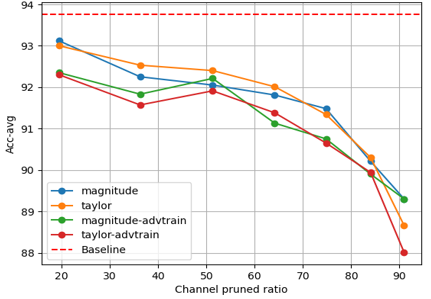
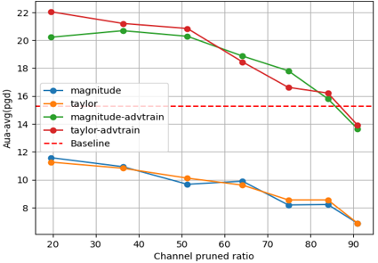
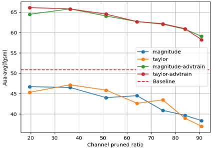
Supporting this observation, Figure 2 compares various pruning methods across multiple architectures, including ResNet-50, MobileViT-xs, and VGG-16, evaluated on CIFAR-10/100 and Tiny-ImageNet datasets(pruning details are in subsection B.1). The results consistently show that while there are slight differences in performance based on the pruning criteria, all methods exhibit a similar recovery in both standard accuracy and robustness after fine-tuning. These findings reinforce our central argument: the key to effective robust pruning lies in designing fine-tuning strategies, rather than focusing solely on the choice of pruning criteria. In this work, we aim to bridge the gap between model compression and adversarial robustness by developing a targeted fine-tuning algorithm that enhances the resilience of pruned networks. Specifically, we introduce Module Robust Pruning and Fine-Tuning (MRPF), a novel metric that adapts the pruning ratio for each layer based on its sensitivity to adversarial attacks. By incorporating adversarial considerations directly into the pruning and fine-tuning process, we ensure that pruned models maintain both efficiency and robustness. Our results demonstrate that this approach enables practical deployment of DNNs that are not only compact but also capable of withstanding adversarial perturbations, thus contributing to the advancement of robust and efficient neural network models.

2 Related Work

2.1 Pruning Neural Networks

Pruning research dates back to 1988 (Hanson and Pratt, 1988), but it gained widespread attention when Han et al. (Han et al., 2015) proposed sparsifying deep models by removing non-significant synapses and then re-training to restore performance. The Pruning After Training (PAT) pipeline is the most popular because it is believed that pretraining a dense network is essential to obtain an efficient subnetwork (Frankle and Carbin, 2018).

Weight importance can be assessed through various metrics, such as the magnitude of the weights. Han et al. (Han et al., 2015) evaluated weight importance by absolute value, while Li et al. (Li et al., 2016) used the l1-norm to score filters. More advanced techniques, such as Discrimination-aware Channel Pruning (DCP) (Zhuang et al., 2018), incorporate loss minimization to identify the most discriminative channels.

The Lottery Ticket Hypothesis (LTH) (Frankle and Carbin, 2018) posits that sparse, independently trainable subnetworks can be found within dense networks. However, later works, including Multi-Prize LTH (Diffenderfer and Kailkhura, 2021), challenge LTH, showing that training settings like learning rate and epochs greatly influence the success of finding such subnetworks.

Recent efforts aim to achieve more precise pruning by leveraging deeper insights into network structure and function. For instance, Group Fisher Pruning (GFP) (Liu et al., 2021) evaluates importance by computing the Fisher information, providing a statistical measure of each parameter’s contribution to the network’s performance. Similarly, techniques like HRank (Lin et al., 2020) use Singular Value Decomposition to rank filters based on the information content of their activations, effectively identifying and removing less informative filters.

2.2 Robustness of Neural Networks

The susceptibility of state-of-the-art DNNs to adversarial attacks was first highlighted by Goodfellow (2014) and Szegedy (2013). Adversarial attacks are subtle manipulations, often undetectable to humans, but can significantly affect model predictions. This vulnerability is particularly concerning in critical applications like autonomous driving and healthcare.

While pruning generally aims to improve efficiency, it often comes at the cost of reduced adversarial robustness (Gui et al., 2019). However, studies such as (Guo et al., 2018; Jordao and Pedrini, 2021) suggest that retraining after pruning can mitigate some of these negative effects. Phan et al. (2022) introduces CSTAR, a framework that integrates low-rankness and adversarial robustness into a unified optimization problem. It proposes an automatic rank selection scheme to avoid manual tuning and demonstrates significant improvements in benign and robust accuracy. These findings emphasize the importance of balancing sparsity, accuracy, and robustness in pruned neural networks.

2.3 Robust Pruning

Recent advancements in pruning and fine-tuning strategies have focused on improving both model efficiency and robustness. Zhu et al. (2023) proposed Module Robust Criticality (MRC) to identify redundant modules in adversarially trained models, followed by Robust Critical Fine-Tuning (RiFT) to enhance generalization while preserving adversarial robustness. Similarly, Bair et al. (2023) introduced Adaptive Sharpness-Aware Pruning (AdaSAP), which optimizes accuracy and robust generalization through adaptive weight perturbations and structured pruning. In contrast, our proposed Module Robust Pruning and Fine-Tuning (MRPF) method aims to dynamically adjust pruning ratios based on each layer’s sensitivity to adversarial perturbations, offering a more fine-grained approach to balancing model efficiency and robustness. By focusing on layer-specific pruning and adversarial sensitivity, MRPF demonstrates significant improvements across diverse datasets and architectures, effectively bridging the gap between pruning and adversarial fine-tuning.

2.4 Fine-tuing after Pruning

Many pruning techniques require retraining the subnetwork after pruning to recover performance (Le and Hua, 2021). This retraining can be done either by fine-tuning the pruned model or training it from scratch, and the choice between these approaches remains a topic of debate (Cheng et al., 2024). Research by Liu et al. (2018) suggests that subnetworks trained from random reinitialization often outperform those fine-tuned from pre-trained models, particularly in architectures like ResNet and VGG on ImageNet. In contrast, Li et al. (2016) demonstrate that fine-tuning yields better results than training from scratch in their experiments. Studies by Gao et al. (2021) emphasize that fine-tuning is critical for achieving superior performance in sparse mobile networks, outperforming models trained from scratch. Additionally, training from scratch typically requires more training steps to reach convergence, making it a less cost-effective option compared to fine-tuning pre-trained models, especially considering comparable training costs (Ye et al., 2020).

3 Proposed Method

Our method addresses the trade-off between model compression and robustness by incorporating adversarial examples into the pruning process. This ensures that even after significant pruning, the model maintains its defense against adversarial attacks. The core idea stems from the observation that robustness is not evenly distributed across layers in a neural network. Some layers contribute more to the model’s adversarial resilience than others. By identifying and retaining these critical layers while pruning the less important ones, we achieve a highly compressed model that preserves its security.

The rationale for this approach is twofold. First, conventional pruning methods often overlook the network’s robustness, leading to compromised security when adversarial examples are introduced. By integrating adversarial sensitivity into the pruning process, we ensure the model retains its ability to resist attacks, even in a more compact form. Second, this method is computationally efficient: instead of treating all layers uniformly, we focus computational resources on the most critical parts of the model. This targeted pruning not only reduces FLOPs but also enhances the network’s efficiency without sacrificing robustness.

3.1 Preliminaries

We define a neural network with $L$ layers, where $N_{i}$ and $N_{i+1}$ represent the number of input and output channels of the $i^{th}$ convolutional layer, respectively. Let $K$ denote the kernel size, and $F_{i,j}\in\mathbb{R}^{N_{i}\times K\times K}$ represent the $j^{th}$ filter in the $i^{th}$ layer. The complete set of filters for the $i^{th}$ layer is denoted by $\{F_{i,j}\}_{j=1}^{N_{i+1}}$ and is parameterized by weights $W(i)\in\mathbb{R}^{N_{i+1}\times N_{i}\times K\times K}$ for all layers $i\in[1,L]$.

For pruning, we partition the filters into two subsets: $F_{pruned}$ for removal and $F_{keep}$ for retention. $F_{keep}$ is defined as the set $\{F_{i,j}|j\in ID(i)\}$, where $ID(i)$ indexes the most critical filters contributing significantly to performance in layer $i$.

Given a dataset $D=\{(x_{i},y_{i})\}_{i=1}^{n}$ and a desired sparsity level $\kappa$ (representing the number of remaining non-zero filters), the objective is to minimize the loss function $\ell(F_{keep};D)$ over the set of retained filters $F_{keep}$, subject to the constraint that the cardinality of $F_{keep}$, denoted $N_{set}(F_{keep})$, does not exceed $\kappa$:

$$\begin{split}\min_{F_{keep}}\ell(F_{keep};D)=\min_{F_{keep}}\frac{1}{n}\sum_{i=1}^{n}\ell(F_{keep};(x_{i},y_{i}))\\ \text{s.t.}\quad N_{set}(F_{keep})\leq\kappa,\quad F\in\mathbb{R}^{N\times K\times K}.\end{split}$$ (1)

The loss function $\ell(\cdot)$ is typically cross-entropy loss. The reduction in FLOPs is measured after each iteration using:

$$P^{\prime}=1-\frac{f_{flop}(N^{\prime})}{f_{flop}(N)}$$ (2)

This indicates the efficiency of pruning compared to the initial target.

3.2 Pruning Method

Generate Adversarial Examples: Adversarial examples $AE$ are generated using an adversarial attack method $AT$ on the training data $D$. These examples are created to exploit the vulnerabilities of the model.

$$AE=AT(D)$$ (3)

The baseline adversarial loss $L_{\text{orig}}$ is computed by evaluating the adversarial examples on the original model:

$$L_{\text{orig}}=L_{\text{adv}}(N(AE),y_{AE})$$ (4)

This step is important because traditional pruning methods rely solely on performance metrics like accuracy. However, in adversarial settings, it is not enough for a pruned model to perform well on clean data—it must also withstand adversarial attacks. By incorporating adversarial examples into the evaluation, we ensure the pruned model is robust across a wider range of inputs.

Perturb Layer Weights: For each layer $l_{i}$, the algorithm perturbs the weights $W_{l_{i}}$ by performing gradient ascent on the adversarial loss. This step measures how sensitive the adversarial loss is to changes in the layer’s parameters. The update rule for the weights is:

$$W_{l_{i}}^{(t+1)}=W_{l_{i}}^{(t)}+\eta\cdot\nabla_{W_{l_{i}}}L_{\text{adv}}(N(W_{l_{i}}^{(t)},X_{\text{adv}}),y_{\text{adv}})$$ (5)

where $\eta$ is the learning rate. After each update, the weights are projected back into a bounded region to satisfy the perturbation constraint:

$$\|W_{l_{i}}^{(t+1)}-W_{l_{i}}^{\text{orig}}\|_{2}\leq\epsilon\cdot\|W_{l_{i}}^{\text{orig}}\|_{2}$$ (6)

Layers that are more sensitive to these perturbations play a larger role in the model’s defense and should be pruned with caution. This step is justified because it allows us to identify the layers that contribute most to adversarial robustness, guiding the pruning process based on the model’s defensive properties rather than arbitrary weight magnitudes.

Calculate Model Robustness Sensitivity (MRS): We define the MRS to quantify the effect of perturbing each layer’s weights on the adversarial loss. It is computed as the difference between the perturbed adversarial loss and the original adversarial loss:

$$\begin{split}\text{MRS}(l_{i})=L_{\text{adv}}(N(W_{l_{i}}^{\text{pert}},AE),y_{AE})\\ -L_{\text{adv}}(N(W_{l_{i}}^{\text{orig}},AE),y_{AE})\end{split}$$ (7)

Layers with higher MRS values are more important for maintaining robustness, and their channels should be retained during pruning. The rationale for using MRS is that it directly ties the pruning decision to the network’s robustness, ensuring that the layers critical for defense are preserved.

Compute Pruning Ratios: The pruning ratios are computed based on the inverse of the MRS values. Layers with lower MRS values (i.e., less critical for robustness) are pruned more aggressively, while layers with higher MRS values are pruned conservatively. This method ensures that pruning is guided by the functional importance of each layer rather than uniformity across the network, optimizing for both model compression and robustness.

The inverse of the MRS values is calculated:

$$\text{InvMRS}(l_{i})=\frac{1}{\text{MRS}(l_{i})+\delta}$$ (8)

where $\delta$ is a small constant to prevent division by zero. The pruning weights are normalized across all layers:

$$w_{i}=\frac{\text{InvMRS}(l_{i})}{\sum_{j}\text{InvMRS}(l_{j})}$$ (9)

The pruning ratio for each layer is scaled by the global pruning ratio $r_{g}$ and capped at the maximum pruning ratio $r_{\text{max}}$:

$$p_{i}=\min(w_{i}\cdot r_{g},\,r_{\text{max}})$$ (10)

Prune the Network: The algorithm prunes each layer by removing the lowest $p_{i}\times k_{i}$ channels based on importance scores (e.g., Taylor (Molchanov et al., 2019)), where $k_{i}$ is the number of channels in layer $l_{i}$. The number of pruned channels is:

$$k_{i}^{\text{pruned}}=\lfloor p_{i}\times k_{i}\rfloor$$ (11)

Fine-tune the Pruned Model: After pruning, the model $N^{\prime}$ is fine-tuned using an augmented dataset $D^{\prime}$ that includes a fraction $r_{AT}$ of newly generated adversarial examples:

$$D^{\prime}=D\cup\left(r_{AT}\times AE^{\prime}\right)$$ (12)

The model is fine-tuned on $D^{\prime}$ until convergence to restore performance and robustness.

The proposed algorithm(see Appendix A), integrated into the Module Robust Pruning and Fine-tuning (MRPF) framework, combines three key criteria—gradient information, loss change after channel removal, and sensitivity to adversarial perturbations—to perform robust channel pruning. By generating adversarial examples and calculating the Model Robustness Sensitivity (MRS), the algorithm dynamically adjusts per-layer pruning ratios based on each layer’s contribution to robustness. This ensures that channels are pruned not only by weight magnitude but also by their functional importance to adversarial resilience. Fine-tuning with adversarial examples restores both accuracy and robustness, making it highly effective for deploying robust and efficient networks.

4 Experiments

In this section, we detail the experimental setup and the results obtained from our model pruning experiments across various architectures and datasets. Our goal is to explore the effects of different pruning strategies on both standard accuracy and adversarial robustness.

We begin by introducing the datasets and baseline architectures utilized for evaluation, followed by the training configurations tailored for pruning.

Finally, the results are presented in terms of key metrics such as test accuracy and adversarial robustness, providing insights into how different pruning strategies affect model performance, particularly when evaluated against adversarial attacks.

4.1 Experimental Setup

Datasets and Baseline Architectures.

We utilize three widely-recognized datasets for our experiments: CIFAR-10/100  (Krizhevsky and Hinton, 2009) and Tiny-ImageNet  (Le and Yang, 2015). Our experiments focus on pruning various network architectures, including VGGNet (Simonyan and Zisserman, 2014), ResNet (He et al., 2016), and MobileViT (Mehta and Rastegari, 2021). These models are pruned using channel compression ratios ranging from 10% to 80%.

Training Settings.

Training followed settings used in (He et al., 2016, 2019; Mehta and Rastegari, 2021), adapted for the pruning context. Models were fine-tuned using SGD with momentum (Sutskever et al., 2013), and Step and cosine annealing learning rate adjustment algorithms were applied, starting from the same initial rate. Step annealing reduces the learning rate (set to 10% of its previous value) at fixed intervals, while cosine annealing follows a smooth reduction pattern based on a cosine function over time.

For pruning comparisons, we evaluated Random (select randomly the index of channels to prune), Hessian, Magnitude, Taylor (Molchanov et al., 2019), and LAMP (Lee et al., 2020) as baselines. For MRPF progress, adversarial examples were generated using FGSM with an attack budget of 2/255, and the adversarial data proportion was set at 20%.(More details are in Appendix B)

Evaluation Matrices.

We calculate the test set accuracy for each standard dataset. For evaluating adversarial robustness, we use PGD-20 (Madry, 2017) and FGSM (Goodfellow, 2014), selecting robust accuracy as the final metric. For PGD-20 and FGSM adversarial attacks, the attack budget $\epsilon$ is set to 8/255, with a step size of 2/255 for PGD-20. We report the average results across three different seeds.

4.2 Main Results

4.2.1 Pruning Criteria Impact

(a) ResNet-50 on CIFAR-10 (Acc)

(b) MobileVit-xs on CIFAR-10 (Acc)

(c) VGG-16 on CIFAR-100 (Acc)

(d) ResNet-50 on CIFAR-10 (PGD Attack)

(e) MobileVit-xs on CIFAR-10 (PGD Attack)

(f) VGG-16 on CIFAR-100 (PGD Attack)

(g) ResNet-50 on CIFAR-10 (FGSM Attack)

(h) MobileVit-xs on CIFAR-10 (FGSM Attack)

(i) VGG-16 on CIFAR-100 (FGSM Attack)

Figure 2: Impact of various pruning criteria on accuracy and robustness across different architectures and datasets. The figures illustrate the performance under different pruning methods (random, magnitude, Hessian, Taylor, LAMP) for ResNet-50, MobileViT-xs, and VGG-16 on CIFAR-10 and CIFAR-100. Regardless of the pruning method, similar accuracy and robustness are achieved after fine-tuning.

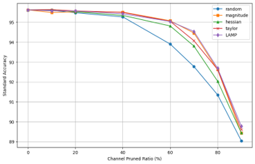
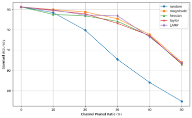
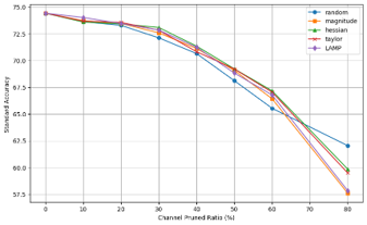
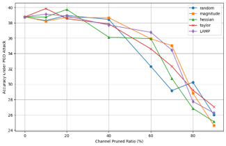
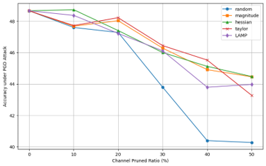
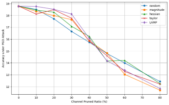
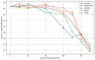
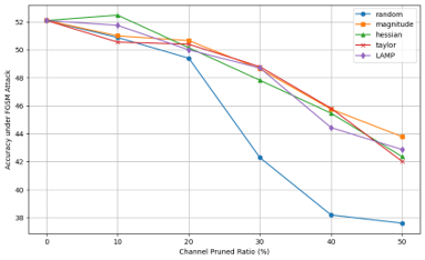
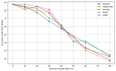
The experimental results, presented in Figure 2, provide several key insights into the relationship between pruning criteria, compression ratios, and the fine-tuning process. Specifically, the choice of pruning criteria—whether based on simple methods like weight magnitude or more advanced approaches such as Hessian or Taylor series approximations—was found to have a limited impact on the final performance of pruned models after fine-tuning. This conclusion held true across all evaluated architectures, including ResNet-50, MobileViT-xs, and VGG-16, as well as across datasets like CIFAR-10 and CIFAR-100. Despite their structural differences, these models exhibited similar recovery in both standard accuracy and adversarial robustness after pruning, irrespective of the specific pruning strategy employed.

Minor Performance Gains at Low Compression Ratios: At low compression ratios (below 50%), pruning often led to slight performance improvements. This can be attributed to the removal of redundant parameters that may have introduced noise, thus making the model more streamlined and efficient. By eliminating these unnecessary elements, the model can potentially reduce overfitting and improve accuracy. These findings suggest that moderate pruning not only reduces model size but can also enhance performance by simplifying the network.

Performance Decline at High Compression Ratios: As the compression ratio increased beyond 60–70%, both accuracy and robustness began to deteriorate across all pruning methods. This decline suggests that the overall compression level, rather than the specific pruning criteria, drives performance loss. At high compression ratios, important parameters are removed, leading to a less accurate model with coarser decision boundaries. This makes the pruned model more prone to errors and more vulnerable to adversarial attacks.

Role of Fine-Tuning in Mitigating Pruning Effects: Fine-tuning was essential in recovering performance, particularly for compression levels up to 50%. Even after pruning, models retained sufficient capacity to re-learn critical patterns and decision boundaries during retraining, restoring both accuracy and robustness. The choice of fine-tuning methods, particularly optimization algorithms and learning rate schedules, played a pivotal role in this recovery. Models pruned with different criteria but fine-tuned in a similar way typically converged to comparable performance, highlighting the dominant influence of fine-tuning.

Limitations at Higher Compression Ratios: Despite the benefits of fine-tuning, its effectiveness wanes as compression ratios exceed 70%. Even the best fine-tuning strategies cannot fully compensate for the loss of key parameters, leading to noticeable declines in both standard accuracy and adversarial robustness. This limitation underscores the inherent trade-off between efficiency and performance: while aggressive pruning reduces model size, it can also compromise the model’s ability to generalize and defend against adversarial perturbations.

Optimization Algorithm Impact: The results in Table 1 highlight the significant impact of the optimization algorithm on pruned model performance. Magnitude-Step consistently outperforms Magnitude-Cosine, especially at higher compression levels, maintaining better accuracy and robustness against adversarial attacks. A similar trend is observed when comparing Random-Step and Random-Cosine, where Step-based approaches show stronger retention of accuracy and robustness under aggressive pruning. These findings underscore that Step-based scheduling consistently yields better results than Cosine-based methods, particularly as the pruning ratio increases.

Table 1: Comparison of Different Optimization Algorithms on ResNet-34-Tiny-ImageNet.

FLOPs(%) $\downarrow$	Magnitude-Step			Magnitude-Cosine
	Acc-avg	Adv${}_{\text{PGD-2}}$	Adv${}_{\text{FGSM}}$	Acc-avg	Adv${}_{\text{PGD-2}}$	Adv${}_{\text{FGSM}}$
0	61.59	11.94	11.73	60.71	10.79	11.87
19.54	62.59	13.58	13.50	61.37	11.69	12.73
51.51	61.93	12.67	12.76	60.48	11.01	12.57
74.92	61.02	13.30	13.14	59.02	9.57	11.80
FLOPs(%) $\downarrow$	Random-Step			Random-Cosine
	Acc-avg	Adv${}_{\text{PGD-2}}$	Adv${}_{\text{FGSM}}$	Acc-avg	Adv${}_{\text{PGD-2}}$	Adv${}_{\text{FGSM}}$
0	61.59	11.94	11.73	60.71	10.79	11.87
19.54	62.76	11.76	12.01	61.95	10.81	12.20
51.51	61.69	12.14	12.08	59.95	10.42	12.10
74.92	59.77	10.84	11.13	57.06	8.89	10.91

In conclusion, while weight importance scoring is often considered pivotal in pruning strategies, the results suggest that effective fine-tuning after pruning is the dominant factor influencing the model’s final performance. This observation underscores the need for a balanced approach to pruning and fine-tuning to maintain both accuracy and robustness, particularly at higher compression levels.

4.2.2 Performance Analysis of MRPF

The results in Table 2(additional results are provided in Appendix C) demonstrate that the Module Robust Pruning and Fine-Tuning (MRPF) framework significantly enhances adversarial robustness while maintaining strong accuracy and computational efficiency across various architectures.

For ResNet-18 on CIFAR-10, MRPF nearly doubled robustness against PGD attacks compared to conventional Taylor pruning, with similar improvements for FGSM attacks. On CIFAR-100, the framework showed comparable gains, more than doubling adversarial robustness for both PGD-2 and FGSM attacks. This underscores MRPF’s effectiveness in protecting critical model parameters against adversarial perturbations.

VGG-16 also benefited greatly from MRPF. On CIFAR-10, robustness against FGSM attacks increased substantially, following the same pattern observed with ResNet-18. CIFAR-100 results confirmed these findings, with MRPF consistently improving the model’s resilience to adversarial attacks over traditional pruning methods.

MRPF not only improved robustness but also maintained strong accuracy and efficiency. In ResNet on CIFAR-10, accuracy improved slightly, with modest FLOPs reduction, while VGG-16 showed stable accuracy and a minor efficiency boost. These results demonstrate that MRPF enhances robustness without significant computational overhead. Furthermore, for more complex architectures like ResNet-50, MRPF effectively preserved and recovered performance post-pruning, highlighting its scalability and suitability for larger networks where balancing robustness and efficiency is crucial.

Additionally, the results suggest that MRPF scales effectively with network complexity, as larger models like ResNet-50 show a greater capacity to retain and recover performance after pruning, indicating that the framework is particularly well-suited for more sophisticated architectures where balancing robustness and efficiency is crucial.

Table 2: Performance of Different Methods and Architectures with FLOPs Reduction for CIFAR-10/100.

Architecture	Method	CIFAR-10				CIFAR-100
		FLOPs(%) $\downarrow$	Std	Adv${}_{\text{PGD-8}}$	Adv${}_{\text{FGSM}}$	FLOPs(%) $\downarrow$	Std	Adv${}_{\text{PGD-2}}$	Adv${}_{\text{FGSM}}$
ResNet-50	Dense	0	95.68	10.09	47.24	0	78.10	17.15	20.82
	Taylor	74.83	94.39	8.06	45.06	84.03	75.32	11.86	18.14
	Taylor + MRPF	74.53	95.04	18.61	72.21	83.41	74.81	31.41	37.52
	Magnitude	74.83	94.74	8.37	45.29	84.03	75.34	12.27	18.93
	Magnitude + MRPF	74.53	95.25	19.38	71.47	83.41	75.16	31.97	37.72
MobileVit-xs	Dense	0	93.13	21.00	52.10	0	70.69	19.03	19.88
	Taylor	74.37	90.44	15.02	40.57	73.83	65.42	15.59	15.21
	Taylor + MRPF	71.51	90.86	25.44	58.01	70.76	64.52	27.73	25.54
	Magnitude	73.46	90.63	16.75	41.92	73.58	65.10	16.37	15.85
	Magnitude + MRPF	70.47	89.87	24.84	57.73	70.91	65.08	27.58	25.72
VGG-16	Dense	0	93.76	15.28	50.87	0	74.6	18.71	24.35
	Taylor	64.14	92.01	9.61	42.61	64.14	68.05	14.30	19.97
	Taylor + MRPF	68.67	91.46	20.71	62.47	62.67	68.37	28.05	35.13
	Magnitude	64.14	91.81	9.89	44.47	64.14	68.75	13.63	19.11
	Magnitude + MRPF	68.67	91.33	19.43	63.13	61.98	68.37	27.31	33.96

4.2.3 Ablation Study

Table 3: Impact of MRPF on Robustness.

Architecture	Method	FLOPs(%) $\downarrow$	Std	Adv${}_{\text{PGD}}$	Adv${}_{\text{FGSM}}$
ResNet-18	Magnitude + AT	51.60	93.8	10.78	66.79
	Magnitude + MRPF	55.63	93.97	21.06	67.21
	Magnitude + AT	91.05	91.68	13.91	62.67
	Magnitude + MRPF	90.73	91.63	15.8	62.79
VGG-16	Magnitude + AT	51.28	92.21	20.28	64.04
	Magnitude + MRPF	54.78	92.22	21.32	64.48
	Magnitude + AT	64.14	91.13	18.86	62.66
	Magnitude + MRPF	68.67	91.33	19.43	63.13

Analysis of Pruning with MRS: Table 3 highlights the benefits of incorporating the Module Robustness Sensitivity (MRS) into the pruning process. When comparing MRPF to the baseline approach, which applies adversarial training (AT) without MRS, we observe a clear improvement in adversarial robustness. Across both ResNet-18 and VGG-16 architectures, MRPF consistently enhances resilience against adversarial attacks, demonstrating its ability to preserve critical parameters essential for maintaining robust decision boundaries.

In addition to improving robustness, MRPF achieves these gains with only minimal changes in standard accuracy and computational efficiency. This indicates that the integration of MRS into the pruning process results in a more balanced trade-off between robustness and efficiency, something that adversarial training alone cannot accomplish.

Table 4: Comparison of Different Adversarial Examples on ResNet-18.

Method	Std	Adv${}_{\text{PGD}}$	Adv${}_{\text{FGSM}}$
FGSM	93.49	20.29	66.35
NIFGSM	93.31	19.77	66.84
VMIFGSM	93.32	19.15	66.85
PGD	93.47	19.34	66.36

Table 5: Comparison of Different Ratios of Adversarial Examples on ResNet-56.

Ratio(%)	Std	Adv${}_{\text{PGD}}$	Adv${}_{\text{FGSM}}$
0	94.31	44.25	52.40
20	93.96	66.81	70.34
50	93.41	67.86	68.89
100	23.00	46.49	44.85

Impact of different Adversarial examples: Under a FLOPs reduction rate of 64.35% and an adversarial budget of 8/255, we assessed the influence of various adversarial example generation methods (FGSM (Goodfellow, 2014), NIFGSM (Lin et al., 2019), VMIFGSM (Wang and He, 2021)), and PGD (Madry, 2017)). As shown in Table 5, the differences in robustness and standard accuracy across these methods are minimal. FGSM showed a slight advantage in robustness, but overall, the variation in adversarial example generation techniques did not significantly impact the final performance, suggesting that the choice of method plays a relatively minor role under these conditions.

Impact of different ratios of Adversarial examples: We investigated the effect of varying the ratio of adversarial examples (from 0% to 100%) on ResNet-56 under a FLOPs reduction rate of 64.36%. The PGD-20 attack was performed with a budget of 2/255, while FGSM used a budget of 8/255.

As shown in Table 5, increasing the adversarial ratio to 20% significantly boosts robustness with minimal impact on standard accuracy. Ratios beyond 50% provide diminishing returns in robustness and a sharp drop in standard accuracy, particularly at 100%, where the accuracy falls drastically to 23%. This suggests that a moderate adversarial ratio offers an optimal balance between maintaining model accuracy and improving robustness.

5 Conclusion and Future Work

In this paper, we demonstrated that fine-tuning plays a dominant role in preserving both accuracy and adversarial robustness in pruned deep neural networks, often outweighing the effects of specific pruning criteria. Our proposed Module Robust Pruning and Fine-Tuning (MRPF) method adaptively adjusts layer-wise pruning ratios based on sensitivity to adversarial attacks, achieving a balance between model efficiency and robustness. Experimental results confirm the effectiveness of this approach in enhancing robustness without significant performance loss. Future work will explore optimal layer-specific compression limits to further improve the balance between compression rates and performance, with a focus on broader architectures and adversarial scenarios.

Appendix A Algorithm of MRPF

The complete algorithm of Module Robust Pruning and Fine-Tuning (MRPF) is presented in Algorithm 1.

Input: Training data $D$; pre-trained neural network $N$ with layers $\{l_{i}\}$, each with $k_{i}$ channels; target global pruning ratio $r_{g}$; max per-layer pruning ratio $r_{\text{max}}$; min per-layer pruning ratio $r_{\text{min}}$; adversarial attack method $AT$; adversarial examples ratio $r_{AT}$; learning rate $\eta$; number of epochs $E$; perturbation limit $\epsilon$; batch size $B$

Output: Pruned and fine-tuned neural network $N^{\prime}$

1

/* 1. Generate Adversarial Examples */

2 Generate adversarial examples: $AE=AT(D)$;

3Compute baseline adversarial loss: $L_{\text{orig}}=\frac{1}{|AE|}\sum_{(x,y)\in AE}\ell(N(x),y)$;

/* 2. Calculate MRS for Each Layer */

4 Initialize $\text{MRS}(l_{i})=0$ for all layers $l_{i}$;

5for each prunable layer $l_{i}$ in $N$ do

6       Clone the network: $N_{i}\leftarrow N$;

7      Enable gradients for $W_{l_{i}}$, freeze others; Store original weights: $W_{l_{i}}^{\text{orig}}\leftarrow W_{l_{i}}$;

8      for epoch $e=1$ to $E$ do

9             for each batch $(X_{\text{adv}},y_{\text{adv}})$ in $AE$ do

10                   Compute loss: $L=-\frac{1}{B}\sum_{b=1}^{B}\ell(N_{i}(X_{\text{adv}}^{(b)}),y_{\text{adv}}^{(b)}))$;

11                  Update weights: $W_{l_{i}}\leftarrow W_{l_{i}}+\eta\nabla_{W_{l_{i}}}L$; Project weights to satisfy: $\frac{\|W_{l_{i}}-W_{l_{i}}^{\text{orig}}\|_{2}}{\|W_{l_{i}}^{\text{orig}}\|_{2}}\leq\epsilon$;

12             end for

13            

14       end for

15      

16      Compute perturbed adversarial loss: $L_{\text{pert}}=\frac{1}{|AE|}\sum_{(x,y)\in AE}\ell(N_{i}(x),y)$;

17      Calculate MRS: $\text{MRS}(l_{i})=L_{\text{pert}}-L_{\text{orig}}$;

18 end for

19

/* 3. Compute Pruning Ratios */

20 Replace any $\text{MRS}(l_{i})\leq 0$ with a small constant $\delta$;

21Collect MRS values: $\text{MRS}_{i}=\text{MRS}(l_{i})$; Ensure non-negative MRS values: $\text{MRS}_{i}=\max(\text{MRS}_{i},\delta)$;

22Compute mean MRS: $\mu_{\text{MRS}}=\frac{1}{L}\sum_{i=1}^{L}\text{MRS}_{i}$; Compute MRS deviation: $\Delta_{i}=\text{MRS}_{i}-\mu_{\text{MRS}}$;

23Normalize deviations to $[-1,1]$: $\Delta_{i}=\frac{\Delta_{i}}{\max_{j}|\Delta_{j}|}$;

24Compute initial pruning ratios: $p_{i}=r_{g}-\Delta_{i}\times(r_{\text{max}}-r_{\text{min}})$;

25Clip pruning ratios to $[r_{\text{min}},r_{\text{max}}]$: $p_{i}=\min\left(\max\left(p_{i},r_{\text{min}}\right),r_{\text{max}}\right)$; Adjust pruning ratios: $p_{i}\leftarrow p_{i}\times\frac{r_{g}}{r_{\text{actual}}}$;

/* 4. Prune the Network */

26 for each layer $l_{i}$ do

27       Prune the lowest $\lfloor p_{i}\times k_{i}\rfloor$ channels based on importance scores;

28 end for

29

/* 5. Fine-tune the Pruned Model */

30 Generate new adversarial examples: $AE^{\prime}=AT(D)$;

31Form augmented dataset: $D^{\prime}=D\cup\left(r_{AT}\times AE^{\prime}\right)$; Fine-tune $N^{\prime}$ on $D^{\prime}$ until convergence;

return Pruned and fine-tuned neural network $N^{\prime}$

Algorithm 1 Module Robust Pruning and Fine-Tuning (MRPF)

Appendix B EXPERIMENT DETAILS

B.1 MRPF Schedule and Settings

CIFAR-10, CIFAR-100  [Krizhevsky and Hinton, 2009], and Tiny-ImageNet [Le and Yang, 2015] are widely-used benchmark datasets for image classification tasks. CIFAR-10 consists of 60,000 32x32 color images across 10 classes, with relatively simple and distinct features. CIFAR-100 is a more complex version, containing the same number of images but spread across 100 classes, introducing greater inter-class similarity. Tiny-ImageNet, a subset of the ImageNet dataset, includes 100,000 images of size 64x64 across 200 classes, offering a more challenging classification task due to its higher number of classes and increased image complexity.

The pruning process in this work combines adversarial training with adaptive pruning to enhance both robustness and efficiency. The process starts by loading a pre-trained model, such as MobileViT-xs  [Mehta and Rastegari, 2021], VGG-16  [Simonyan and Zisserman, 2014] , or a ResNet variant  [He et al., 2016], trained on datasets like CIFAR-10, CIFAR-100, or Tiny-ImageNet. These models serve as the baseline for subsequent pruning and fine-tuning.

For CIFAR-10 and CIFAR-100, once the pre-trained model is loaded, adversarial examples are generated using FGSM [Goodfellow, 2014] attacks with an epsilon value of 2/255. These adversarial examples are used to evaluate the model’s performance, establishing an initial robustness baseline.

Next, neuron importance is computed using pruning criteria such as Taylor expansion  [Molchanov et al., 2019] or Magnitude pruning. In this work, Magnitude pruning is predominantly used for the CIFAR-10/100 experiments. The per-layer pruning ratios are computed based on the importance scores and normalized globally across the network to ensure balance. To avoid over-pruning, the maximum pruning ratio for any layer is capped at 80%, and the global pruning ratio is controlled to achieve an optimal balance between performance and efficiency.

The pruning process is iterative: neurons are pruned layer by layer based on their importance scores, followed by network fine-tuning after each pruning step. The fine-tuning process integrates adversarial training with a 0.2 adversarial ratio to ensure that the pruned network retains its robustness while improving efficiency. During fine-tuning, clean and adversarial examples are combined to maintain performance under various conditions. The SGD optimizer is employed during fine-tuning, with the learning rate following a cosine annealing schedule, starting at a maximum of 0.02 and gradually decaying to $1e^{-4}$ over the 90 epochs.

For Tiny-ImageNet, the pruning procedure involves certain adjustments to accommodate the larger dataset and model complexity. Adversarial examples are generated using FGSM attacks with an epsilon value of 2/255. The batch size is reduced to 128 to meet the higher computational demands, and the learning rate is initially set to 0.1 before decaying to $1e^{-4}$ over 90 epochs following a cosine annealing schedule.

The fine-tuning process plays a critical role in ensuring that the pruned models recover both accuracy and robustness. The networks are fine-tuned using the SGD optimizer with a cosine annealing learning rate decay, starting from 0.02 for CIFAR datasets and 0.1 for Tiny-ImageNet, decaying to a minimum of $1e^{-4}$ over 90 epochs. Throughout this phase, adversarial training is maintained with a 0.2 adversarial ratio, and FGSM attacks with an epsilon of 2/255 are used to generate adversarial examples.

By the end of this iterative pruning and fine-tuning process, the models retain competitive accuracy and robustness across CIFAR and Tiny-ImageNet datasets. This approach achieves significant reductions in computational complexity without compromising adversarial robustness.

B.2 Adversarial Example Generation Methods

FGSM [Goodfellow, 2014] is a single-step attack that generates adversarial examples by adding a perturbation to the input in the direction that maximizes the loss. Given a neural network model $N$ with parameters $\theta$, an input sample $\mathbf{x}$, and its true label $y$, the adversarial example $\mathbf{x}^{\text{adv}}$ is generated as:

$$\mathbf{x}^{\text{adv}}=\mathbf{x}+\epsilon\cdot\text{sign}\left(\nabla_{\mathbf{x}}\mathcal{L}\left(N(\mathbf{x};\theta),y\right)\right),$$ (13)

where:

• $\epsilon$ is the perturbation magnitude, controlling the strength of the attack.

• $\mathcal{L}(\cdot,\cdot)$ is the loss function used for training (e.g., cross-entropy loss).

• $\nabla_{\mathbf{x}}\mathcal{L}\left(N(\mathbf{x};\theta),y\right)$ is the gradient of the loss with respect to the input $\mathbf{x}$.

• $\text{sign}(\cdot)$ denotes the element-wise sign function.

The perturbation $\epsilon\cdot\text{sign}\left(\nabla_{\mathbf{x}}\mathcal{L}\right)$ is designed to maximize the loss, effectively causing the model to misclassify the input while keeping the perturbation minimal and often imperceptible to humans.

PGD [Madry, 2017] is an iterative attack that refines the adversarial example over multiple steps, making it a stronger attack than FGSM. Starting from the original input $\mathbf{x}^{0}=\mathbf{x}$, PGD updates the adversarial example by:

$$\mathbf{x}^{t+1}=\Pi_{\mathcal{B}(\mathbf{x},\epsilon)}\left(\mathbf{x}^{t}+\alpha\cdot\text{sign}\left(\nabla_{\mathbf{x}}\mathcal{L}\left(N(\mathbf{x}^{t};\theta),y\right)\right)\right),$$ (14)

for $t=0,1,\dots,T-1$, where:

• $\alpha$ is the step size for each iteration.

• $T$ is the total number of iterations.

• $\Pi_{\mathcal{B}(\mathbf{x},\epsilon)}(\cdot)$ is the projection operator that ensures $\mathbf{x}^{t+1}$ stays within the $\epsilon$-ball $\mathcal{B}(\mathbf{x},\epsilon)$ around the original input $\mathbf{x}$ and within the valid data range (e.g., $[0,1]$ for image data).

After $T$ iterations, the final adversarial example is $\mathbf{x}^{\text{adv}}=\mathbf{x}^{T}$. The PGD attack can be seen as a multi-step variant of FGSM, repeatedly applying small perturbations and projecting back into the feasible set to find a more effective adversarial example.

Implementation Details

In our experiments, as described in Appendix B.1, we use FGSM with $\epsilon=\frac{2}{255}$ to generate adversarial examples for both CIFAR-10 and CIFAR-100 datasets. For Tiny-ImageNet, we use the same $\epsilon$ value to maintain consistency across experiments.

For FGSM, since it is a single-step method, we set the step size $\alpha$ equal to $\epsilon$. For PGD, which we use in ablation studies to test the robustness of our pruned models, we set the step size $\alpha=\frac{\epsilon}{T}$, where $T$ is the number of iterations (we set 20 in the experiments). This ensures that the total perturbation remains within the $\epsilon$ constraint.

Integrating adversarial examples generated by FGSM and PGD into our pruning process serves multiple purposes:

• Evaluating Robustness: By assessing the model’s performance on adversarial examples, we establish a baseline for robustness, ensuring that pruning does not degrade this critical property.

• Guiding Pruning Decisions: The gradients computed during adversarial example generation highlight the model’s sensitive features. By focusing on these gradients, we can identify which neurons or channels are crucial for robustness and should be retained.

• Adversarial Training: Incorporating adversarial examples into the fine-tuning process helps the pruned model recover and maintain robustness against attacks, as discussed in Section B.1.

B.3 Importance Score Calculation

In our pruning process, we compute the importance of each channel using mainly two criteria: Magnitude importance and Taylor importance. These methods help identify which channels contribute most to the model’s performance and should be retained during pruning.

B.3.1 Magnitude Importance

Magnitude importance measures the significance of each channel based on the magnitude of its weights. For a given convolutional layer $l_{i}$ with weights $W_{l_{i}}\in\mathbb{R}^{N_{i+1}\times N_{i}\times K\times K}$ (where $N_{i}$ and $N_{i+1}$ are the numbers of input and output channels, and $K$ is the kernel size), the importance score $I_{l_{i},j}$ for output channel $j$ is calculated as:

$$I_{l_{i},j}=\sum_{k=1}^{N_{i}}\sum_{u=1}^{K}\sum_{v=1}^{K}\left|W_{l_{i},j,k,u,v}\right|^{p}$$ (15)

where:

• $W_{l_{i},j,k,u,v}$ is the weight connecting the $k^{\text{th}}$ input channel to the $j^{\text{th}}$ output channel at position $(u,v)$ in layer $l_{i}$.

• $p$ is the norm degree, typically set to 2 (i.e., L2-norm).

This method sums the $p$-th power of the absolute values of all weights in output channel $j$, providing a scalar importance score. Channels with higher magnitude importance are considered more significant and are less likely to be pruned.

B.3.2 Taylor Importance

Taylor importance estimates the contribution of each channel to the loss function using a first-order Taylor expansion [Molchanov et al., 2019]. For output channel $j$ in layer $l_{i}$, the importance score $I_{l_{i},j}$ is calculated as:

$$I_{l_{i},j}=\sum_{k=1}^{N_{i}}\sum_{u=1}^{K}\sum_{v=1}^{K}\left|W_{l_{i},j,k,u,v}\cdot\frac{\partial\ell}{\partial W_{l_{i},j,k,u,v}}\right|$$ (16)

where:

• $\ell$ is the loss function (e.g., cross-entropy loss).

• $\frac{\partial\ell}{\partial W_{l_{i},j,k,u,v}}$ is the gradient of the loss with respect to the weight $W_{l_{i},j,k,u,v}$.

By considering both the weights and their gradients, Taylor importance captures how sensitive the loss is to changes in each weight. This method effectively identifies channels that, when pruned, would have a significant impact on the loss, allowing us to preserve critical channels during pruning.

B.3.3 Normalization and Pruning Decision

After computing the importance scores using either method, we normalize the scores to ensure fair comparison across layers. The normalization can be performed using methods such as:

$$\tilde{I}_{l_{i},j}=\frac{I_{l_{i},j}}{\text{mean}(\mathbf{I}_{l_{i}})}$$ (17)

where $\mathbf{I}_{l_{i}}$ is the vector of importance scores for all channels in layer $l_{i}$. This normalization helps in balancing the pruning process across different layers with varying importance score distributions.

Channels with lower normalized importance scores $\tilde{I}_{l_{i},j}$ are considered less critical and are pruned first. By applying these importance criteria, we effectively reduce the model size while maintaining performance and robustness.

B.4 Model Robustness Sensitivity Calculation

In this appendix, we provide additional details on the calculation of Model Robustness Sensitivity (MRS) used in our pruning algorithm, as outlined in Section 3. The MRS quantifies the impact of perturbing each layer’s weights on the adversarial loss, guiding the pruning process to preserve layers that are crucial for robustness.

B.4.1 Implementation Details

To compute the MRS for each layer, we perform the following steps:

1. Perturbing Layer Weights: For each prunable layer $l_{i}$, we perform gradient ascent on the adversarial loss to perturb its weights $W_{l_{i}}$, while keeping the weights of other layers fixed. The perturbation is constrained to a small norm $\epsilon$ relative to the original weights, as described in Equation (4) in the main text.

2. Computing Perturbed Adversarial Loss: After perturbing $W_{l_{i}}$, we evaluate the adversarial loss $L_{\text{adv}}$ on the adversarial examples $AE$ using the network with perturbed weights in layer $l_{i}$.

3. Calculating MRS: The MRS for layer $l_{i}$ is calculated as the difference between the perturbed adversarial loss and the original adversarial loss $L_{\text{orig}}$, as defined in Equation (5) in the main text.

4. Adjustment of MRS Values: To handle any non-positive MRS values, we replace any $\text{MRS}(l_{i})\leq 0$ with a small positive constant $\delta$ to prevent numerical issues during pruning ratio computation.

B.4.2 Pruning Ratio Computation

Following the calculation of MRS for all layers, we compute the pruning ratios $p_{i}$ for each layer. Instead of directly using the inverse of MRS values as in Equation (6) in the main text, we normalize the MRS deviations to ensure the pruning ratios are within the desired range. The steps are as follows:

1. Compute the mean MRS: $\mu_{\text{MRS}}=\frac{1}{L}\sum_{i=1}^{L}\text{MRS}(l_{i})$.

2. Compute the deviation of MRS values from the mean: $\Delta_{i}=\text{MRS}(l_{i})-\mu_{\text{MRS}}$.

3. Normalize the deviations to the range $[-1,1]$: $\Delta_{i}=\frac{\Delta_{i}}{\max_{j}|\Delta_{j}|}$.

4. Compute the initial pruning ratios: $p_{i}=r_{g}-\Delta_{i}\times(r_{\text{max}}-r_{\text{min}})$.

5. Clip the pruning ratios to be within $[r_{\text{min}},r_{\text{max}}]$.

6. Adjust the pruning ratios to match the target global pruning ratio $r_{g}$: $p_{i}\leftarrow p_{i}\times\frac{r_{g}}{r_{\text{actual}}}$, where $r_{\text{actual}}=\frac{1}{L}\sum_{i=1}^{L}p_{i}$.

This method ensures that layers with higher MRS values (more important for robustness) receive lower pruning ratios, while layers with lower MRS values are pruned more aggressively.

B.4.3 Additional Notes

• The perturbation limit $\epsilon$ is set to a small value (e.g., $\epsilon=8/255$) to ensure that the weight perturbations remain within a reasonable range.

• The learning rate $\eta$ and the number of epochs $E$ for the gradient ascent are chosen to effectively perturb the weights without excessive computation.

• The small constant $\delta$ used to adjust non-positive MRS values is set to a small positive value (e.g., $\delta=1\times 10^{-6}$).

Appendix C ADDITIONAL RESULTS

C.1 Comparison of MRPF Results Across Different Datasets

Table 6: Performance of Different Methods and Architectures with FLOPs Reduction for CIFAR-10 and CIFAR-100.

Architecture	Method	CIFAR-10				CIFAR-100
		FLOPs(%) $\downarrow$	Std	Adv${}_{\text{PGD-8}}$	Adv${}_{\text{FGSM}}$	FLOPs(%) $\downarrow$	Std	Adv${}_{\text{PGD-2}}$	Adv${}_{\text{FGSM}}$
ResNet-18	Dense	0	92.11	12.45	40.02	0	75.42	16.55	18.54
	Taylor	51.60	93.86	10.78	49.19	64.35	72.61	15.42	17.78
	Taylor + MRPF	55.63	93.57	20.76	66.38	69.06	74.28	33.99	35.71
	Magnitude	51.60	93.9	10.78	48.36	64.35	72.42	15.13	17.94
	Magnitude + MRPF	55.63	93.97	21.06	67.21	69.06	72.83	33.86	36.33
	Taylor	91.05	92.19	6.41	42.64	84.18	71.34	13.78	15.06
	Taylor + MRPF	90.73	91.76	14.24	60.89	83.15	71.16	30.42	33.31
	Magnitude	91.05	92.12	6.13	42.69	84.18	70.15	13.28	15.53
	Magnitude + MRPF	90.73	91.63	15.80	62.79	83.15	70.25	27.82	31.24
VGG-16	Dense	0	93.76	15.28	50.87	0	74.6	18.71	24.35
	Taylor	51.28	92.01	10.11	45.84	51.27	70.85	16.09	22.39
	Taylor + MRPF	54.78	91.67	22.11	63.61	54.78	69.73	28.84	35.60
	Magnitude	51.28	92.05	9.67	43.99	51.27	70.78	14.02	19.64
	Magnitude + MRPF	54.78	92.22	21.32	64.48	54.21	69.73	28.69	36.12

Table 7: Performance of Different Fine-tuning Methods on Mobilevit with FLOPs Reduction for CIFAR-10 and CIFAR-100.

Architecture	Method	CIFAR-10				CIFAR-100
		FLOPs(%) $\downarrow$	Std	Adv${}_{\text{PGD-8}}$	Adv${}_{\text{FGSM}}$	FLOPs(%) $\downarrow$	Std	Adv${}_{\text{PGD-2}}$	Adv${}_{\text{FGSM}}$
	Dense	0	93.13	21.01	52.10	0	70.69	19.03	19.88
	Taylor	64.31	91.14	16.29	43.24	51.85	68.82	16.85	17.12
	Taylor + AT	64.31	90.34	22.33	57.38	51.91	67.15	29.82	27.89
	Taylor + MRPF	60.53	91.72	26.2	62.91	59.8	67.68	29.62	27.85
	Magnitude	63.25	91.32	16.97	45.47	50.80	69.43	18.10	18.85
	Magnitude + AT	63.25	90.4	22.80	55.66	50.80	68.37	30.18	28.18
MobileVit-xs	Magnitude + MRPF	59.38	91.85	27.61	62.91	59.56	67.45	29.86	27.61
	Taylor	83.63	88.09	15.10	39.80	73.83	65.42	15.59	15.21
	Taylor + AT	83.63	87.09	18.4	50.16	73.90	62.49	24.84	23.28
	Taylor + MRPF	79.95	89.13	23.54	55.73	70.76	64.52	27.73	25.54
	Magnitude	82.84	89.07	14.88	37.64	73.58	65.10	16.37	15.85
	Magnitude + AT	82.84	87.16	18.23	50.26	73.58	62.93	26.27	24.82
	Magnitude + MRPF	79.95	89.12	23.62	54.33	70.91	65.08	27.58	25.72

The results presented in Table 6, Table 7, and Table 8 illustrate the performance of the Module Robust Pruning and Fine-Tuning (MRPF) framework across CIFAR-10, CIFAR-100, and Tiny-ImageNet datasets. These results highlight MRPF’s ability to consistently enhance adversarial robustness while maintaining strong accuracy across various architectures and datasets.

CIFAR-10 and CIFAR-100: As shown in Table 6, for ResNet-18 and VGG-16, MRPF consistently improved adversarial robustness, especially against FGSM and PGD attacks, compared to baseline Taylor and Magnitude pruning methods. On CIFAR-10, ResNet-18 exhibited a significant improvement in adversarial accuracy under PGD-8 attacks, increasing from 10.78% (Taylor) to 20.76% (Taylor + MRPF), representing an improvement of nearly 92.5%. In CIFAR-100, MRPF delivered an even larger relative increase in adversarial accuracy under PGD-2 attacks, from 15.42% (Taylor) to 33.99% (Taylor + MRPF), achieving a 120% improvement, despite the higher complexity of CIFAR-100. These results suggest that MRPF effectively maintains robustness even under more challenging classification tasks like CIFAR-100.

For VGG-16, MRPF preserved high standard accuracy (91.67% in CIFAR-10) while delivering substantial gains in adversarial robustness. For example, under FGSM attacks on CIFAR-10, adversarial accuracy increased from 45.84% to 63.61%, marking a 38.7% improvement. On CIFAR-100, a similar trend was observed with improvements in adversarial accuracy under PGD-2 attacks, highlighting MRPF’s ability to handle both accuracy and robustness effectively in different scenarios.

MobileViT-xs: In more complex architectures like MobileViT-xs, MRPF demonstrated even stronger improvements, particularly at higher FLOP reductions, as detailed in Table 7. For CIFAR-10, adversarial accuracy under PGD-8 attacks improved from 16.97% (Magnitude pruning) to 27.61% (Magnitude + MRPF), reflecting a 62.7% increase. On CIFAR-100, adversarial accuracy under FGSM attacks rose from 18.85% to 29.86%, a 58.4% improvement. These results indicate that MRPF is especially effective in complex architectures like MobileViT-xs, which benefit more from adaptive pruning strategies due to their inherent complexity. This analysis suggests that MRPF not only preserves standard accuracy but also substantially improves adversarial robustness, particularly in more complex networks like MobileViT-xs. The adaptive nature of MRPF allows it to handle architectures that are more sensitive to pruning, further supporting its broader applicability across diverse network types.

Table 8: Performance of Different Fine-tuning Methods on ResNet with FLOPs Reduction for Tiny-ImageNet.

Architecture	Method	FLOPs(%) $\downarrow$	Std	Adv${}_{\text{PGD-2}}$	Adv${}_{\text{FGSM}}$
	Dense	0	62.40	8.28	9.88
	Taylor	74.83	57.01	7.46	10.09
	Taylor + AT	74.83	57.52	21.30	26.64
	Taylor + MRPF	72.62	59.63	25.26	28.53
	Magnitude	74.83	57.64	8.11	10.48
	Magnitude + AT	74.83	57.56	21.25	25.68
ResNet-50	Magnitude + MRPF	72.62	58.69	23.94	26.70
	Taylor	84.03	56.29	8.67	11.31
	Taylor + AT	84.03	55.55	19.32	24.34
	Taylor + MRPF	88.77	55.96	20.82	25.32
	Magnitude	84.03	56.59	6.01	8.44
	Magnitude + AT	84.03	55.76	19.78	24.86
	Magnitude + MRPF	88.77	55.34	20.47	25.78

Tiny-ImageNet: For ResNet-50 on Tiny-ImageNet, the experimental results reported in Table 8 show that MRPF significantly improves adversarial robustness while maintaining a high standard accuracy, even under aggressive pruning. Under FGSM attacks, MRPF improved adversarial accuracy from 10.09% (Taylor) to 28.53% (Taylor + MRPF), achieving a remarkable 182.7% improvement. Standard accuracy remained relatively strong at 59.63%. These results demonstrate that MRPF can adapt effectively to larger and more complex datasets, providing notable gains in adversarial robustness without sacrificing performance.

Cross-Dataset Comparison and Additional Insights: When comparing the performance of MRPF across datasets, it becomes evident that the framework consistently improves adversarial robustness while maintaining strong standard accuracy. For larger datasets like Tiny-ImageNet, the improvements in robustness were more substantial, likely due to the increased pruning flexibility afforded by deeper architectures such as ResNet-50. The adversarial accuracy gains under FGSM attacks were particularly pronounced, showing greater improvement in Tiny-ImageNet (182.7%) compared to CIFAR-10 (67.7%) or CIFAR-100 (58.4%).

Moreover, this analysis underscores an interesting observation: both dataset complexity and network architecture influence the efficacy of MRPF. More complex datasets and architectures offer greater opportunities for MRPF to enhance adversarial robustness while maintaining performance. The higher the complexity of the dataset (Tiny-ImageNet $>$ CIFAR-100 $>$ CIFAR-10) and architecture (MobileViT-xs $>$ ResNet-50 $>$ ResNet-18), the more pronounced the improvements in both adversarial and standard accuracy. This can be attributed to the larger capacity and flexibility of more complex models, which allow MRPF to prune more aggressively while preserving critical features. In challenging datasets like Tiny-ImageNet, MRPF can better focus the model on robustness-related features by pruning less critical neurons, leading to more significant robustness and performance gains.

In summary, MRPF not only enhances adversarial robustness across a variety of datasets and architectures but also shows scalability in maintaining accuracy and performance. The framework’s effectiveness is particularly evident in complex architectures and larger datasets, making it a robust solution for real-world applications where both robustness and computational efficiency are critical.

C.2 Optimization Algorithm Impact

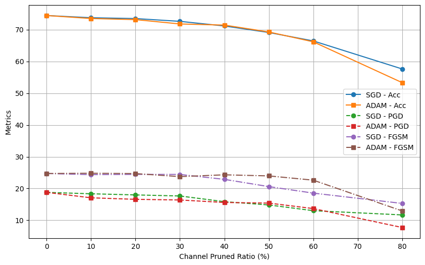
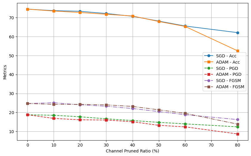
The figures 3(a) and 3(b) highlight the substantial impact of optimizer choice on the performance of pruned models, particularly in the context of adversarial robustness. In both random pruning and magnitude pruning, models optimized with Stochastic Gradient Descent (SGD) consistently outperform those using the ADAM optimizer across a range of channel pruning ratios. This trend is evident not only in terms of standard accuracy but also in adversarial robustness under PGD and FGSM attacks.

As seen in the figures, as the pruning ratio increases from 0% to 80%, the performance gap between SGD and ADAM becomes more pronounced. Specifically, SGD-optimized models maintain higher accuracy and robustness at aggressive pruning levels (e.g., 80% pruning). For instance, in magnitude pruning, SGD sustains a better adversarial accuracy under PGD attacks, reducing the performance degradation that ADAM suffers at higher pruning levels.

The effectiveness of SGD in preserving model robustness can be attributed to its better generalization capabilities, which are particularly important when the model capacity is reduced through pruning. In contrast, ADAM’s adaptive nature may lead to overfitting on smaller, less expressive pruned models, causing a more significant drop in both standard accuracy and adversarial robustness. These findings suggest that optimizer selection is a critical factor in ensuring that pruned models maintain strong performance, especially under adversarial settings.

(a) Random Pruning with SGD and ADAM on VGG-16-CIFAR-100

(b) Magnitude Pruning with SGD and ADAM on VGG-16-CIFAR-100

Figure 3: Impact of different optimizers (SGD and ADAM) on pruned models for VGG-16-CIFAR-100 under different pruning strategies. The left figure shows random pruning, and the right figure shows magnitude pruning.

C.3 Original and Pruned Network Structures

The following outlines the original structure of the CifarResNet model before pruning. The model starts with a convolutional layer followed by several residual blocks (BasicBlock) arranged in four sequential layers. The network culminates with a linear layer for classification. The original model contains approximately 556.65 million MACs (Multiply-Accumulate Operations) and 11.17 million parameters. After pruning, the number of MACs is reduced to 51.57 million, representing a 90.73% reduction, while the parameter count is reduced to 1.74 million, reflecting an 84.42% reduction.

C.3.1 Original CifarResNet Structure:

CifarResNet(
  (conv1): Conv2d(3, 64, kernel_size=(3, 3), stride=(1, 1), padding=(1, 1), bias=False)
  (bn1): BatchNorm2d(64, eps=1e-05, momentum=0.1, affine=True, track_running_stats=True)

  (layer1): Sequential(
    (0): BasicBlock(
      (conv1): Conv2d(64, 64, kernel_size=(3, 3), stride=(1, 1), padding=(1, 1), bias=False)
      (bn1): BatchNorm2d(64, eps=1e-05, momentum=0.1, affine=True, track_running_stats=True)
      (conv2): Conv2d(64, 64, kernel_size=(3, 3), stride=(1, 1), padding=(1, 1), bias=False)
      (bn2): BatchNorm2d(64, eps=1e-05, momentum=0.1, affine=True, track_running_stats=True)
      (shortcut): Sequential()
    )
    (1): BasicBlock(
      (conv1): Conv2d(64, 64, kernel_size=(3, 3), stride=(1, 1), padding=(1, 1), bias=False)
      (bn1): BatchNorm2d(64, eps=1e-05, momentum=0.1, affine=True, track_running_stats=True)
      (conv2): Conv2d(64, 64, kernel_size=(3, 3), stride=(1, 1), padding=(1, 1), bias=False)
      (bn2): BatchNorm2d(64, eps=1e-05, momentum=0.1, affine=True, track_running_stats=True)
      (shortcut): Sequential()
    )
  )

  (layer2): Sequential(
    (0): BasicBlock(
      (conv1): Conv2d(64, 128, kernel_size=(3, 3), stride=(2, 2), padding=(1, 1), bias=False)
      (bn1): BatchNorm2d(128, eps=1e-05, momentum=0.1, affine=True, track_running_stats=True)
      (conv2): Conv2d(128, 128, kernel_size=(3, 3), stride=(1, 1), padding=(1, 1), bias=False)
      (bn2): BatchNorm2d(128, eps=1e-05, momentum=0.1, affine=True, track_running_stats=True)
      (shortcut): Sequential(
        (0): Conv2d(64, 128, kernel_size=(1, 1), stride=(2, 2), bias=False)
        (1): BatchNorm2d(128, eps=1e-05, momentum=0.1, affine=True, track_running_stats=True)
      )
    )
    (1): BasicBlock(
      (conv1): Conv2d(128, 128, kernel_size=(3, 3), stride=(1, 1), padding=(1, 1), bias=False)
      (bn1): BatchNorm2d(128, eps=1e-05, momentum=0.1, affine=True, track_running_stats=True)
      (conv2): Conv2d(128, 128, kernel_size=(3, 3), stride=(1, 1), padding=(1, 1), bias=False)
      (bn2): BatchNorm2d(128, eps=1e-05, momentum=0.1, affine=True, track_running_stats=True)
      (shortcut): Sequential()
    )
  )

  (layer3): Sequential(
    (0): BasicBlock(
      (conv1): Conv2d(128, 256, kernel_size=(3, 3), stride=(2, 2), padding=(1, 1), bias=False)
      (bn1): BatchNorm2d(256, eps=1e-05, momentum=0.1, affine=True, track_running_stats=True)
      (conv2): Conv2d(256, 256, kernel_size=(3, 3), stride=(1, 1), padding=(1, 1), bias=False)
      (bn2): BatchNorm2d(256, eps=1e-05, momentum=0.1, affine=True, track_running_stats.True)
      (shortcut): Sequential(
        (0): Conv2d(128, 256, kernel_size=(1, 1), stride=(2, 2), bias=False)
        (1): BatchNorm2d(256, eps=1e-05, momentum=0.1, affine=True, track_running_stats.True)
      )
    )
    (1): BasicBlock(
      (conv1): Conv2d(256, 256, kernel_size=(3, 3), stride=(1, 1), padding=(1, 1), bias=False)
      (bn1): BatchNorm2d(256, eps=1e-05, momentum=0.1, affine=True, track_running_stats.True)
      (conv2): Conv2d(256, 256, kernel_size=(3, 3), stride=(1, 1), padding=(1, 1), bias=False)
      (bn2): BatchNorm2d(256, eps=1e-05, momentum=0.1, affine=True, track_running_stats.True)
      (shortcut): Sequential()
    )
  )

  (layer4): Sequential(
    (0): BasicBlock(
      (conv1): Conv2d(256, 512, kernel_size=(3, 3), stride=(2, 2), padding=(1, 1), bias=False)
      (bn1): BatchNorm2d(512, eps=1e-05, momentum=0.1, affine=True, track_running_stats.True)
      (conv2): Conv2d(512, 512, kernel_size=(3, 3), stride=(1, 1), padding=(1, 1), bias=False)
      (bn2): BatchNorm2d(512, eps=1e-05, momentum=0.1, affine=True, track_running_stats.True)
      (shortcut): Sequential(
        (0): Conv2d(256, 512, kernel_size=(1, 1), stride=(2, 2), bias=False)
        (1): BatchNorm2d(512, eps=1e-05, momentum=0.1, affine=True, track_running_stats.True)
      )
    )
    (1): BasicBlock(
      (conv1): Conv2d(512, 512, kernel_size=(3, 3), stride=(1, 1), padding=(1, 1), bias=False)
      (bn1): BatchNorm2d(512, eps=1e-05, momentum=0.1, affine=True, track_running_stats.True)
      (conv2): Conv2d(512, 512, kernel_size=(3, 3), stride=(1, 1), padding=(1, 1), bias=False)
      (bn2): BatchNorm2d(512, eps=1e-05, momentum=0.1, affine=True, track_running_stats.True)
      (shortcut): Sequential()
    )
  )
  (linear): Linear(in_features=512, out_features=10, bias=True)
)

C.3.2 Pruned CifarResNet Structure:

CifarResNet(
  (conv1): Conv2d(3, 12, kernel_size=(3, 3), stride=(1, 1), padding=(1, 1), bias=False)
  (bn1): BatchNorm2d(12, eps=1e-05, momentum=0.1, affine=True, track_running_stats.True)

  (layer1): Sequential(
    (0): BasicBlock(
      (conv1): Conv2d(12, 12, kernel_size=(3, 3), stride=(1, 1), padding=(1, 1), bias=False)
      (bn1): BatchNorm2d(12, eps=1e-05, momentum=0.1, affine=True, track_running_stats.True)
      (conv2): Conv2d(12, 12, kernel_size=(3, 3), stride=(1, 1), padding=(1, 1), bias=False)
      (bn2): BatchNorm2d(12, eps=1e-05, momentum=0.1, affine=True, track_running_stats.True)
      (shortcut): Sequential()
    )
    (1): BasicBlock(
      (conv1): Conv2d(12, 12, kernel_size=(3, 3), stride=(1, 1), padding=(1, 1), bias=False)
      (bn1): BatchNorm2d(12, eps=1e-05, momentum=0.1, affine=True, track_running_stats.True)
      (conv2): Conv2d(12, 12, kernel_size=(3, 3), stride=(1, 1), padding=(1, 1), bias=False)
      (bn2): BatchNorm2d(12, eps=1e-05, momentum=0.1, affine=True, track_running_stats.True)
      (shortcut): Sequential()
    )
  )

  (layer2): Sequential(
    (0): BasicBlock(
      (conv1): Conv2d(12, 25, kernel_size=(3, 3), stride=(2, 2), padding=(1, 1), bias=False)
      (bn1): BatchNorm2d(25, eps=1e-05, momentum=0.1, affine=True, track_running_stats.True)
      (conv2): Conv2d(25, 25, kernel_size=(3, 3), stride=(1, 1), padding=(1, 1), bias=False)
      (bn2): BatchNorm2d(25, eps=1e-05, momentum=0.1, affine=True, track_running_stats.True)
      (shortcut): Sequential(
        (0): Conv2d(12, 25, kernel_size=(1, 1), stride=(2, 2), bias=False)
        (1): BatchNorm2d(25, eps=1e-05, momentum=0.1, affine=True, track_running_stats.True)
      )
    )
    (1): BasicBlock(
      (conv1): Conv2d(25, 25, kernel_size=(3, 3), stride=(1, 1), padding=(1, 1), bias=False)
      (bn1): BatchNorm2d(25, eps=1e-05, momentum=0.1, affine=True, track_running_stats.True)
      (conv2): Conv2d(25, 25, kernel_size=(3, 3), stride=(1, 1), padding=(1, 1), bias=False)
      (bn2): BatchNorm2d(25, eps=1e-05, momentum=0.1, affine=True, track_running_stats.True)
      (shortcut): Sequential()
    )
  )

  (layer3): Sequential(
    (0): BasicBlock(
      (conv1): Conv2d(25, 63, kernel_size=(3, 3), stride=(2, 2), padding=(1, 1), bias=False)
      (bn1): BatchNorm2d(63, eps=1e-05, momentum=0.1, affine=True, track_running_stats.True)
      (conv2): Conv2d(63, 51, kernel_size=(3, 3), stride=(1, 1), padding=(1, 1), bias=False)
      (bn2): BatchNorm2d(51, eps=1e-05, momentum=0.1, affine=True, track_running_stats.True)
      (shortcut): Sequential(
        (0): Conv2d(25, 51, kernel_size=(1, 1), stride=(2, 2), bias=False)
        (1): BatchNorm2d(51, eps=1e-05, momentum=0.1, affine=True, track_running_stats.True)
      )
    )
    (1): BasicBlock(
      (conv1): Conv2d(51, 251, kernel_size=(3, 3), stride=(1, 1), padding=(1, 1), bias=False)
      (bn1): BatchNorm2d(251, eps=1e-05, momentum=0.1, affine=True, track_running_stats.True)
      (conv2): Conv2d(251, 51, kernel_size=(3, 3), stride=(1, 1), padding=(1, 1), bias=False)
      (bn2): BatchNorm2d(51, eps=1e-05, momentum=0.1, affine=True, track_running_stats.True)
      (shortcut): Sequential()
    )
  )

  (layer4): Sequential(
    (0): BasicBlock(
      (conv1): Conv2d(51, 483, kernel_size=(3, 3), stride=(2, 2), padding=(1, 1), bias=False)
      (bn1): BatchNorm2d(483, eps=1e-05, momentum=0.1, affine=True, track_running_stats.True)
      (conv2): Conv2d(483, 102, kernel_size=(3, 3), stride=(1, 1), padding=(1, 1), bias=False)
      (bn2): BatchNorm2d(102, eps=1e-05, momentum=0.1, affine=True, track_running_stats.True)
      (shortcut): Sequential(
        (0): Conv2d(51, 102, kernel_size=(1, 1), stride=(2, 2), bias=False)
        (1): BatchNorm2d(102, eps=1e-05, momentum=0.1, affine=True, track_running_stats.True)
      )
    )
    (1): BasicBlock(
      (conv1): Conv2d(102, 417, kernel_size=(3, 3), stride=(1, 1), padding=(1, 1), bias=False)
      (bn1): BatchNorm2d(417, eps=1e-05, momentum=0.1, affine=True, track_running_stats.True)
      (conv2): Conv2d(417, 102, kernel_size=(3, 3), stride=(1, 1), padding=(1, 1), bias.False)
      (bn2): BatchNorm2d(102, eps=1e-05, momentum=0.1, affine=True, track_running.stats.True)
      (shortcut): Sequential()
    )
  )

  (linear): Linear(in_features=102, out_features=10, bias=True)
)

References

- Simonyan and Zisserman [2014] Karen Simonyan and Andrew Zisserman. Very deep convolutional networks for large-scale image recognition. arXiv preprint arXiv:1409.1556, 2014.
- Devlin et al. [2018] Jacob Devlin, Ming-Wei Chang, Kenton Lee, and Kristina Toutanova. Bert: Pre-training of deep bidirectional transformers for language understanding. In Proceedings of the 2019 Conference of the North American Chapter of the Association for Computational Linguistics: Human Language Technologies, dec 2018. doi:10.18653/v1/n19-1423. URL http://dx.doi.org/10.18653/v1/n19-1423.
- Han et al. [2015] Song Han, Jeff Pool, John Tran, and William Dally. Learning both weights and connections for efficient neural network. Advances in neural information processing systems, 28, 2015.
- He et al. [2019] Yang He, Ping Liu, Ziwei Wang, Zhilan Hu, and Yi Yang. Filter pruning via geometric median for deep convolutional neural networks acceleration. In Proceedings of the IEEE/CVF conference on computer vision and pattern recognition, pages 4340–4349, 2019.
- Wu et al. [2016] Jiaxiang Wu, Cong Leng, Yuhang Wang, Qinghao Hu, and Jian Cheng. Quantized convolutional neural networks for mobile devices. In Proceedings of the IEEE conference on computer vision and pattern recognition, pages 4820–4828, 2016.
- Hinton [2015] Geoffrey Hinton. Distilling the knowledge in a neural network. arXiv preprint arXiv:1503.02531, 2015.
- Yin et al. [2021] Miao Yin, Yang Sui, Siyu Liao, and Bo Yuan. Towards efficient tensor decomposition-based dnn model compression with optimization framework. In Proceedings of the IEEE/CVF Conference on Computer Vision and Pattern Recognition, pages 10674–10683, 2021.
- Sun et al. [2024] Mingjie Sun, Zhuang Liu, Anna Bair, and J Zico Kolter. A simple and effective pruning approach for large language models. ICLR, 2024.
- Hanson and Pratt [1988] Stephen Hanson and Lorien Pratt. Comparing biases for minimal network construction with back-propagation. Advances in Neural Information Processing Systems, 1, 1988.
- Frankle and Carbin [2018] Jonathan Frankle and Michael Carbin. The lottery ticket hypothesis: Finding sparse, trainable neural networks. arXiv preprint arXiv:1803.03635, 2018.
- Li et al. [2016] Hao Li, Asim Kadav, Igor Durdanovic, Hanan Samet, and Hans Peter Graf. Pruning filters for efficient convnets. arXiv preprint arXiv:1608.08710, 2016.
- Zhuang et al. [2018] Zhuangwei Zhuang, Mingkui Tan, Bohan Zhuang, Jing Liu, Yong Guo, Qingyao Wu, Junzhou Huang, and Jinhui Zhu. Discrimination-aware channel pruning for deep neural networks. Advances in neural information processing systems, 31, 2018.
- Diffenderfer and Kailkhura [2021] James Diffenderfer and Bhavya Kailkhura. Multi-prize lottery ticket hypothesis: Finding accurate binary neural networks by pruning a randomly weighted network. arXiv preprint arXiv:2103.09377, 2021.
- Liu et al. [2021] Liyang Liu, Shilong Zhang, Zhanghui Kuang, Aojun Zhou, Jing-Hao Xue, Xinjiang Wang, Yimin Chen, Wenming Yang, Qingmin Liao, and Wayne Zhang. Group fisher pruning for practical network compression. In International Conference on Machine Learning, pages 7021–7032. PMLR, 2021.
- Lin et al. [2020] Mingbao Lin, Rongrong Ji, Yan Wang, Yichen Zhang, Baochang Zhang, Yonghong Tian, and Ling Shao. Hrank: Filter pruning using high-rank feature map. In Proceedings of the IEEE/CVF conference on computer vision and pattern recognition, pages 1529–1538, 2020.
- Goodfellow [2014] Ian J Goodfellow. Explaining and harnessing adversarial examples. arXiv preprint arXiv:1412.6572, 2014.
- Szegedy [2013] C Szegedy. Intriguing properties of neural networks. arXiv preprint arXiv:1312.6199, 2013.
- Gui et al. [2019] Shupeng Gui, Haotao Wang, Haichuan Yang, Chen Yu, Zhangyang Wang, and Ji Liu. Model compression with adversarial robustness: A unified optimization framework. Advances in Neural Information Processing Systems, 32, 2019.
- Guo et al. [2018] Yiwen Guo, Chao Zhang, Changshui Zhang, and Yurong Chen. Sparse dnns with improved adversarial robustness. Advances in neural information processing systems, 31, 2018.
- Jordao and Pedrini [2021] Artur Jordao and Hélio Pedrini. On the effect of pruning on adversarial robustness. In Proceedings of the IEEE/CVF International Conference on Computer Vision, pages 1–11, 2021.
- Phan et al. [2022] Huy Phan, Miao Yin, Yang Sui, Bo Yuan, and S. Zonouz. Cstar: Towards compact and structured deep neural networks with adversarial robustness. In AAAI Conference on Artificial Intelligence, 2022. URL https://api.semanticscholar.org/CorpusID:254246536.
- Zhu et al. [2023] Kaijie Zhu, Xixu Hu, Jindong Wang, Xing Xie, and Ge Yang. Improving generalization of adversarial training via robust critical fine-tuning. In Proceedings of the IEEE/CVF International Conference on Computer Vision, pages 4424–4434, 2023.
- Bair et al. [2023] Anna Bair, Hongxu Yin, Maying Shen, Pavlo Molchanov, and Jose Alvarez. Adaptive sharpness-aware pruning for robust sparse networks. arXiv preprint arXiv:2306.14306, 2023.
- Le and Hua [2021] Duong H Le and Binh-Son Hua. Network pruning that matters: A case study on retraining variants. arXiv preprint arXiv:2105.03193, 2021.
- Cheng et al. [2024] Hongrong Cheng, Miao Zhang, and Javen Qinfeng Shi. A survey on deep neural network pruning: Taxonomy, comparison, analysis, and recommendations. IEEE Transactions on Pattern Analysis and Machine Intelligence, 2024.
- Liu et al. [2018] Zhuang Liu, Mingjie Sun, Tinghui Zhou, Gao Huang, and Trevor Darrell. Rethinking the value of network pruning. arXiv preprint arXiv:1810.05270, 2018.
- Gao et al. [2021] Shangqian Gao, Feihu Huang, Weidong Cai, and Heng Huang. Network pruning via performance maximization. In Proceedings of the IEEE/CVF Conference on Computer Vision and Pattern Recognition, pages 9270–9280, 2021.
- Ye et al. [2020] Mao Ye, Chengyue Gong, Lizhen Nie, Denny Zhou, Adam Klivans, and Qiang Liu. Good subnetworks provably exist: Pruning via greedy forward selection. In International Conference on Machine Learning, pages 10820–10830. PMLR, 2020.
- Molchanov et al. [2019] Pavlo Molchanov, Arun Mallya, Stephen Tyree, Iuri Frosio, and Jan Kautz. Importance estimation for neural network pruning. In Proceedings of the IEEE/CVF conference on computer vision and pattern recognition, pages 11264–11272, 2019.
- Krizhevsky and Hinton [2009] A. Krizhevsky and G. Hinton. Learning multiple layers of features from tiny images. Master’s thesis, Department of Computer Science, University of Toronto, 2009.
- Le and Yang [2015] Ya Le and Xuan Yang. Tiny imagenet visual recognition challenge. CS 231N, 7(7):3, 2015.
- He et al. [2016] Kaiming He, Xiangyu Zhang, Shaoqing Ren, and Jian Sun. Identity mappings in deep residual networks. In Computer Vision–ECCV 2016: 14th European Conference, Amsterdam, The Netherlands, October 11–14, 2016, Proceedings, Part IV 14, pages 630–645. Springer, 2016.
- Mehta and Rastegari [2021] Sachin Mehta and Mohammad Rastegari. Mobilevit: light-weight, general-purpose, and mobile-friendly vision transformer. arXiv preprint arXiv:2110.02178, 2021.
- Sutskever et al. [2013] Ilya Sutskever, James Martens, George Dahl, and Geoffrey Hinton. On the importance of initialization and momentum in deep learning. In International conference on machine learning, pages 1139–1147. PMLR, 2013.
- Lee et al. [2020] Jaeho Lee, Sejun Park, Sangwoo Mo, Sungsoo Ahn, and Jinwoo Shin. Layer-adaptive sparsity for the magnitude-based pruning. arXiv preprint arXiv:2010.07611, 2020.
- Madry [2017] Aleksander Madry. Towards deep learning models resistant to adversarial attacks. arXiv preprint arXiv:1706.06083, 2017.
- Lin et al. [2019] Jiadong Lin, Chuanbiao Song, Kun He, Liwei Wang, and John E Hopcroft. Nesterov accelerated gradient and scale invariance for adversarial attacks. arXiv preprint arXiv:1908.06281, 2019.
- Wang and He [2021] Xiaosen Wang and Kun He. Enhancing the transferability of adversarial attacks through variance tuning. In Proceedings of the IEEE/CVF conference on computer vision and pattern recognition, pages 1924–1933, 2021.