On the Influence of Shape, Texture and Color for Learning Semantic Segmentation
Abstract
In recent years, a body of works has emerged, studying shape and texture biases of off-the-shelf pre-trained deep neural networks (DNN) for image classification. These works study how much a trained DNN relies on image cues, predominantly shape and texture. In this work, we switch the perspective, posing the following questions: What can a DNN learn from each of the image cues, i.e., shape, texture and color, respectively? How much does each cue influence the learning success? And what are the synergy effects between different cues? Studying these questions sheds light upon cue influences on learning and thus the learning capabilities of DNNs. We study these questions on semantic segmentation which allows us to address our questions on pixel level. To conduct this study, we develop a generic procedure to decompose a given dataset into multiple ones, each of them only containing either a single cue or a chosen mixture. This framework is then applied to two real-world datasets, Cityscapes and PASCAL Context, and a synthetic data set based on the CARLA simulator. We learn the given semantic segmentation task from these cue datasets, creating cue experts. Early fusion of cues is performed by constructing appropriate datasets. This is complemented by a late fusion of experts which allows us to study cue influence location-dependent on pixel level. Our study on three datasets reveals that neither texture nor shape clearly dominate the learning success, however a combination of shape and color but without texture achieves surprisingly strong results. Our findings hold for convolutional and transformer backbones. In particular, qualitatively there is almost no difference in how both of the architecture types extract information from the different cues.
I Introduction
Visual perception relies on visual stimuli, so-called visual cues, providing information about the perceived scene. Visual environments offer multiple cues about a scene, and observers need to assess the reliability of each cue to integrate the information effectively [1]. To recognize and distinguish objects, for example, their shape and texture provide complementary cues. In cognitive science and psychology the influence of different cues and their combinations for human perception is addressed in various studies [2, 1, 3]. Given the widespread use of deep neural networks (DNNs) for automatically extracting semantic information from scenes, it is important to investigate 1) how these models process and rely on different types of cue information, as well as 2) what they are able to learn when only having access to specific cues. With respect to the first question several hypotheses about dominating cue exploitation (cue biases) of trained convolutional neural networks (CNNs) were formulated and supported by experimental results for image classification tasks [4, 5, 6]. Early in the evolution of CNNs a shape bias was hypothesized, stating that representations of CNN outputs seem to relate to human perceptual shape judgement [7]. Even though this suggests that CNNs tend to base their prediction on shape information, this is only valid on a local perspective [8] and not an intrinsic property [9]. On the contrary, multiple studies were performed on ImageNet-trained CNNs [10], indicating that those CNNs have a bias towards texture [4, 8, 11]. To reveal biases in trained DNNs, cue conflicts are often generated [4, 12]. To this end, a style transfer with a texture image of one class, e.g. showing an animal’s fur or skin, is applied to an ImageNet image representing a different class.
In summary, previous studies 1) mostly study the biases of trained DNNs w.r.t. to image cues and their influence on the networks robustness [4, 13, 14, 15], 2) often rely on style transfer or similar image manipulations to test for biases [16, 5, 17], and 3) largely focus on image classification DNNs [11, 18, 6].
In this work, we present a study that is novel in all three aspects. 1) We switch the perspective, studying how much influence different image cues (and arbitrary combinations of those) have on the learning success of DNNs. 2) We do not rely on style transfer but rather utilize and develop a set of methods, combining them into a generic procedure to derive any desired cue combination of shape, texture and color from a given dataset, cf. fig. 1. 3) We lift our study to the task of semantic segmentation. This opens up paths to completely new studies as it allows for the decomposition of datasets into arbitrary combinations of cues and enables more fine-grained analyses such as image-location-dependent cue influences.
Our study setup serves as basis to train expert networks exclusively relying on a specific cue or cue combination. We perform an in-depth behavioral analysis of CNNs and transformers on three different semantic segmentation datasets, namely Cityscapes [19], PASCAL Context [20] and a synthetic one recorded with the CARLA driving simulator [21]. Our study brings the different cue and cue combination influences on DNN learning into an order. It turns out that neither texture nor shape clearly dominate in terms of learning success. However, a combination of shape and color achieves surprisingly strong results. These findings hold for CNNs and transformers. In particular, qualitatively there is almost no difference in how both architecture types extract information from the different cues, i.e., the choice of backbone has almost no impact on the order of the cue influences. Additionally, by a pixel-wise late fusion of cue (combination) experts, we study the role of each pixel for cue influences, showing that small objects and pixels at object borders are dominantly better predicted by shape experts. Our contributions are summarized as follows:
-
•
We provide a generic procedure to derive cue combination datasets from a given semantic segmentation dataset. In particular, we provide a method to derive texture-only datasets.
-
•
Our general setup allows to study disentangled image cues, down to the detail degree of brightness-only. We perform an in-depth analysis with up to learned cue combination experts per dataset and several late fusion models, contributing the first cue influence study in semantic segmentation. Additionally, we include transformers that are so far underresearched in the broader context of cue influences.
-
•
While previous studies report strong biases of ImageNet-trained DNNs towards texture under style transfer, our study reveals that for real-world data shape and texture are equally important cues for successful learning. The role of the cues varies across classes and image location, but not w.r.t. choosing between CNNs and transformers.
Our code including the data generation procedure will be publicly available soon.
II Related Work
Cue biases and cue decompositions are pivotal concepts in understanding how neural networks interpret visual information. We start by reviewing existing approaches of cues bias analyses in classification, followed by methods to decompose or manipulate data to allow for investigations on different cues. We conclude by addressing the underexplored area of texture and shape biases in semantic segmentation.
Shape and Texture Biases in Image Classification
DNNs learn unintended cues that help to solve the given task but limit their generalization capability [22]. In [4] it was measured whether the shape or the texture cue dominates the decision process of an ImageNet-trained classification CNN by inferring images with conflicting cues (e.g. shape of a cat combined with the skin of an elephant), revealing that ImageNet pre-training leads to a texture bias. Technically, [4] stylize images via style transfer to create cue conflict images. This was also adopted by [16] and [5]. In the latter work, the bias is computed on a per-neuron level. [18] showed that the selection of data and the nature of the task influence the cue biases learned by a CNN. Experiments in [14, 23, 6, 24] demonstrate that transformers exhibit a shape bias in classification tasks, which is attributed to their content-dependent receptive field [14]. Our focus differs in two key aspects: 1) we study cue influences on learning success rather than biases, 2) we consider the task of semantic segmentation instead of image classification.
Data Manipulation for Bias Investigation
To examine the influence of cues, datasets are manipulated by either artificially combining cues to induce conflicts [8, 4, 23, 25] or by selectively removing specific cues from the data [17, 26]. To remove all but the shape cue, edge maps [8, 27, 23], contour maps [8], silhouettes [8] or texture reduction methods [17, 28] are used. Patch shuffling has been proposed to remove the shape cue but preserve the texture [11, 29, 17]. In contrast to classification, data preparation is more complex for semantic segmentation as multiple objects and classes are present in the input which differ in their cues. In particular semantic segmentation on texture-only data is challenging [30]. Removing shape by dividing and shuffling an image as used by [17] for classification compromises semantic integrity of the image and disrupts the segmentation task. Therefore, we propose an alternative method for extracting texture from the dataset, which is sufficiently flexible to generate new segmentation tasks using in-domain textures from the original dataset.
Shape and Texture Biases in Image Segmentation
Up to now, a limited number of works studied shape and texture biases beyond image classification. In [16], for image classification, images are stylized using a second image from the same dataset. For semantic segmentation, only a specific object rather than the full image is used as texture source to perform style transfer. The stylized data is added to the training data to debias the CNN and increase its robustness. Similarly, [25] stylize data to analyze the robustness of instance segmentation networks under randomized texture. Additionally, an object-centric and a background-centric stylization are used for this study. In [26], the change in shape bias of semantic segmentation networks is studied under varying cues in data. The experiments on datasets with a limited number of images and classes reveal that CNNs prioritize non-shape cues if multiple cues are present. [13] propose to colorize images with respect to the class IDs to reduce the influence of texture during training to prevent texture bias and thereby improving robustness of the trained model. In [28], an anisotropic diffusion image processing method is used for removing texture from images. Based on that the texture bias is studied and also reduced. All works mentioned in this paragraph study or reduce biases of DNNs in image segmentation. To the best of our knowledge, the present work is the first one to switch the perspective and study the influence of cues and cue combinations on learning success in semantic segmentation DNNs. This is done on complex datasets with at least classes, by which we obtain different insights.
III Cue Decomposition and Cue Expert Fusion
In this section we introduce the different methods that extract image cues and cue combinations from a given base dataset (original dataset with all cues), from which we train cue and cue combination experts.
Color (C) Cue Extraction
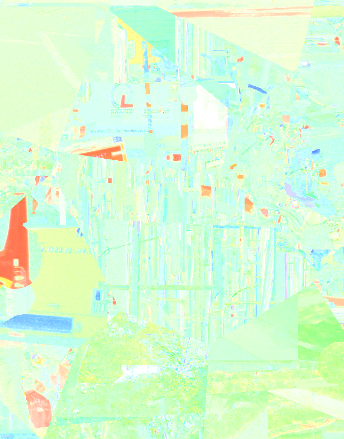
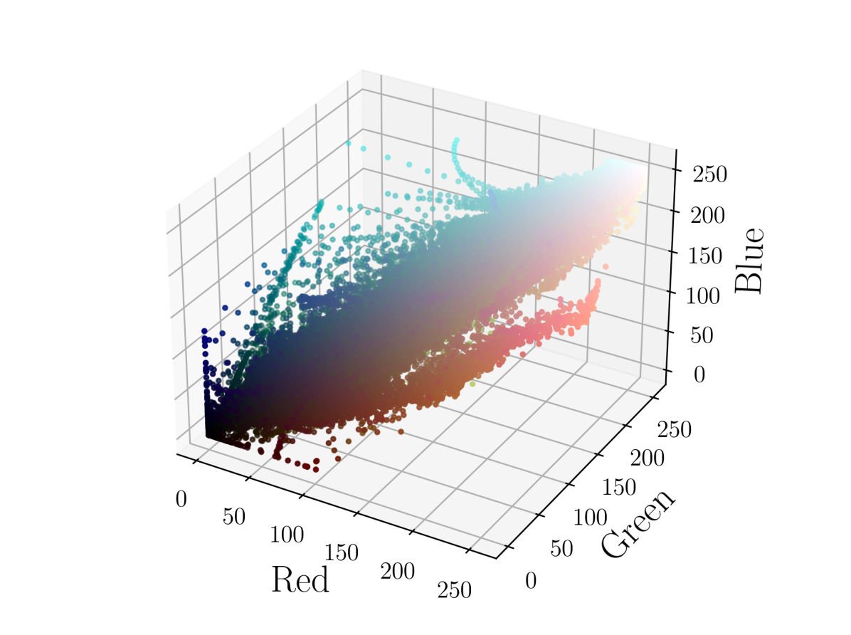
Most cue extractions presented in this work modify the base dataset. In order to isolate the color information, we do not modify the base dataset but constrain the cue expert, i.e., the neural network, to process a single pixel’s color values via -convolutions. This prevents the model from learning spatial patterns such as shapes or textures. Furthermore, we decompose color into two components: its gray value (V) and its chromatic value (HS) by switching to the HSV color space and discarding the value channel. Gray values are obtained by averaging or maximizing RGB channels to extract the degree of darkness or lightness of a given color. In what follows, we use the shorthand C=V+HS to refer to the respective cues.
Texture (T) Cue Extraction
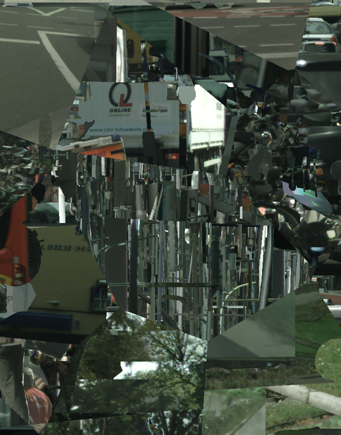
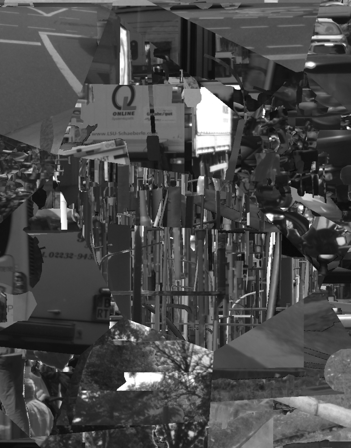
The texture dataset is constructed in three main steps: 1) texture is extracted by cropping object patches using semantic segmentation masks; 2) therefrom, for each class a mosaic image is created by stitching image patches of that class in an overlapping manner; and 3) a new semantic segmentation task is constructed via Voronoi diagrams where each cell is randomly assigned a class and filled with a cutout of the mosaic image corresponding to that class. Figure 2 illustrates this process.
Shape (S) Cue Extraction
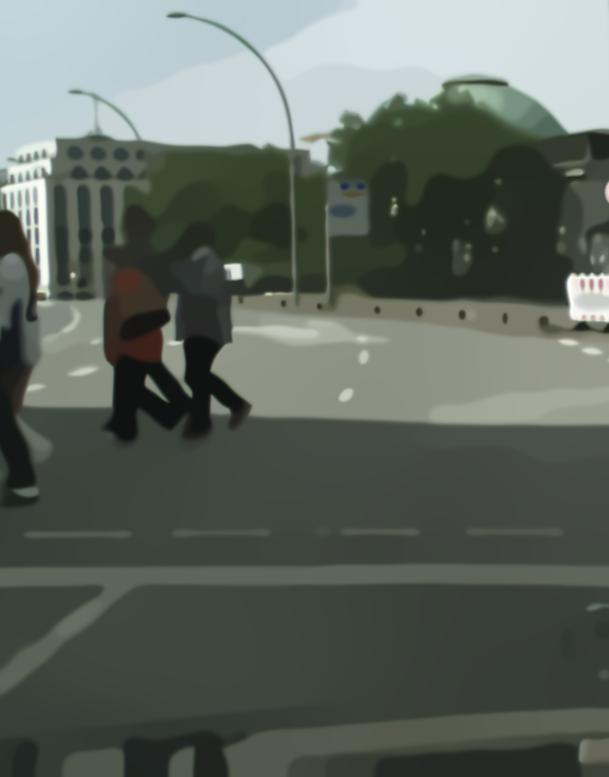
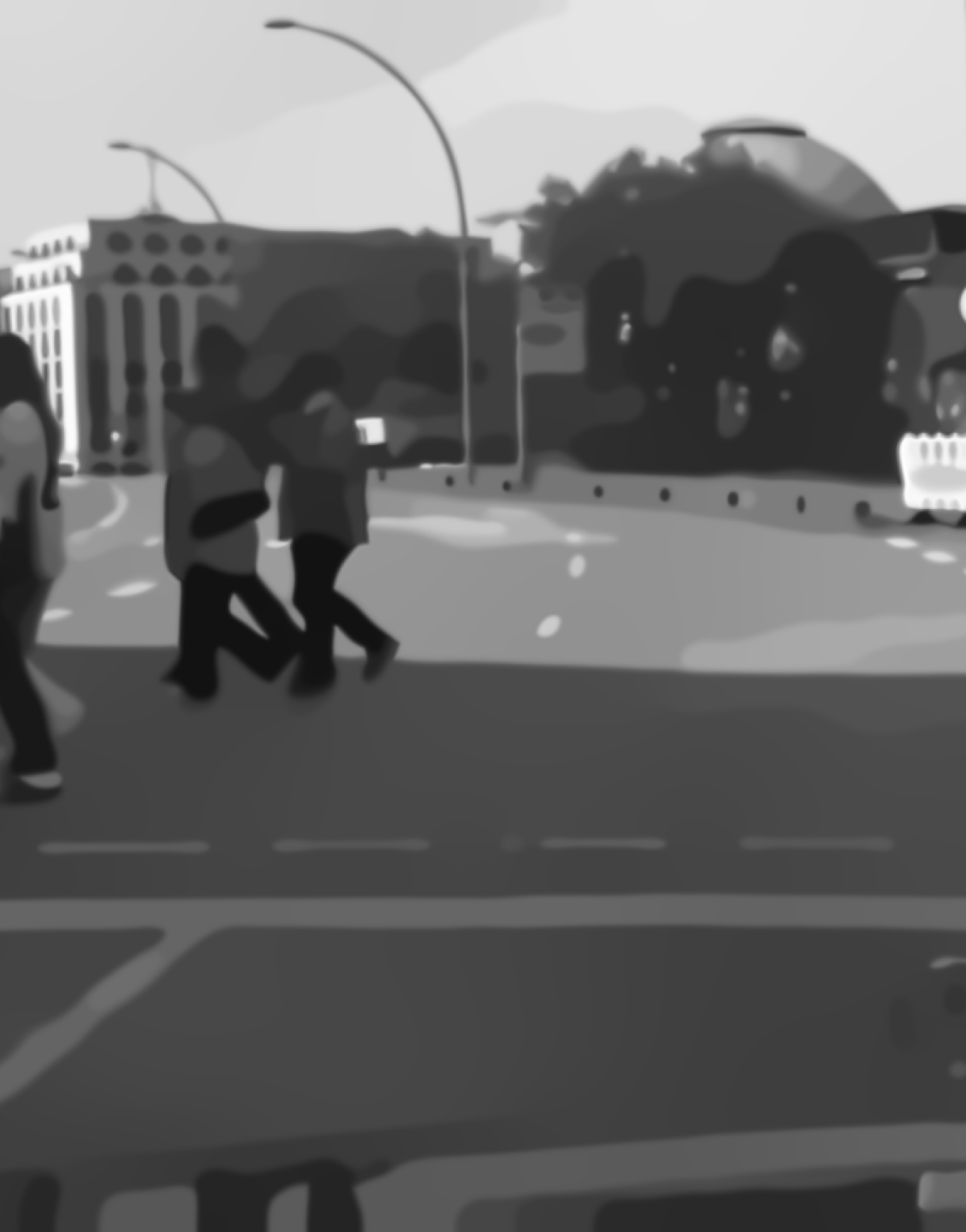
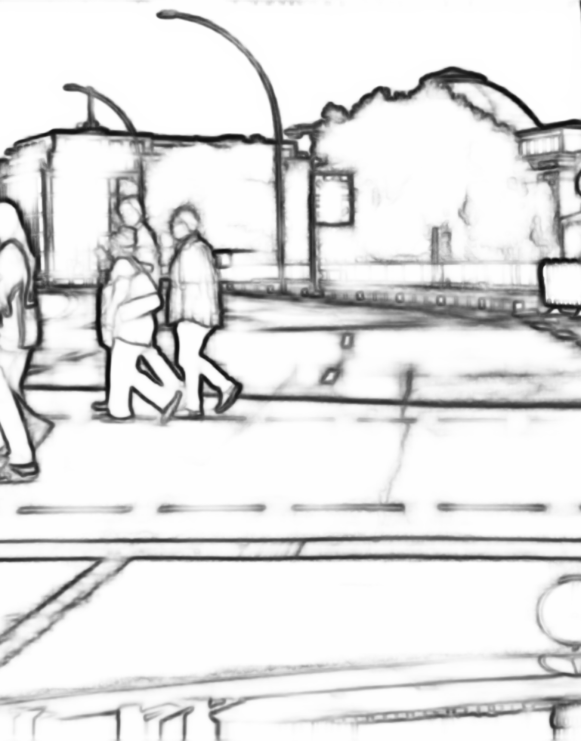
The shape of an object can be described in multiple ways [31], defined by the object with unrecognizable/removed texture or by the object defining edges. To this end, we consider two shape extraction methods: Holistically-nested edge detection (HED) [32] and a variation of Edge Enhancing Diffusion (EED) [28]. HED approximately extracts the object defining edges based on a fully convolutional network which has learned to predict a dense edge map through end-to-end training and nested multiscale feature learning. HED approximates the S cue. In contrast, EED diminishes texture through diffusion along small color gradients in a given image. The diffusion process follows a partial-differential-equation formulation. As it preserves color, it extracts the cues S+V+HS, and analogously to the treatment of the C cue provides the cues S+V as well.
Texture-free Image Data from CARLA ()
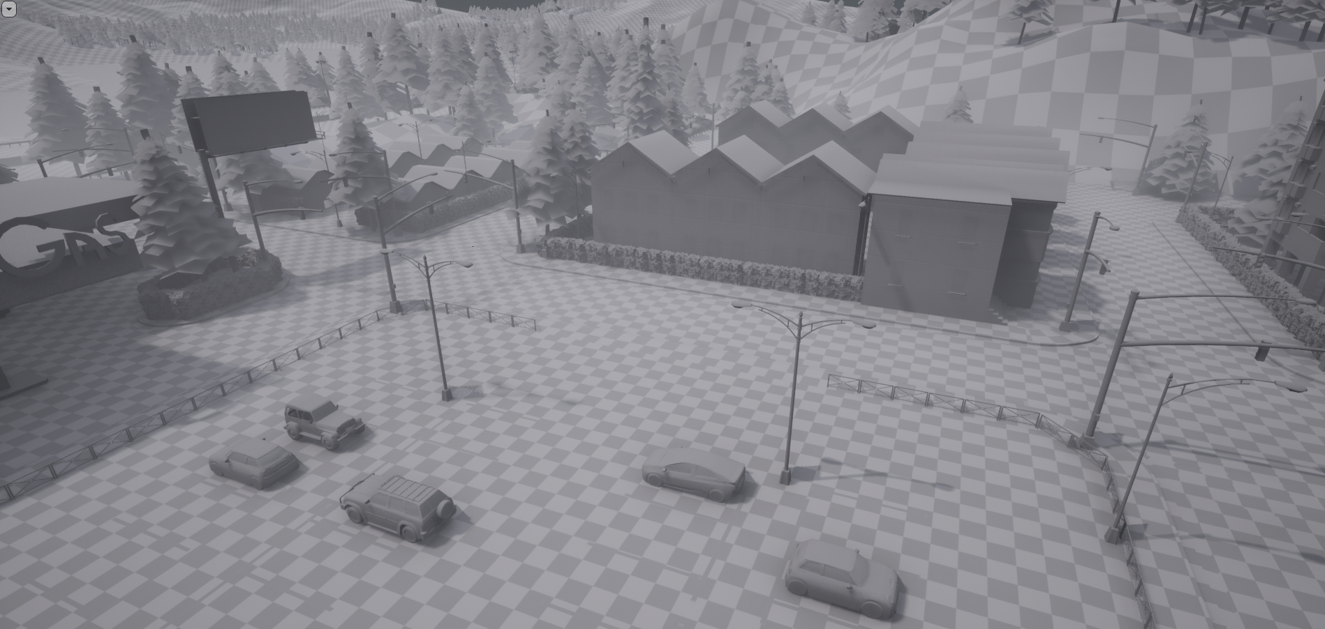
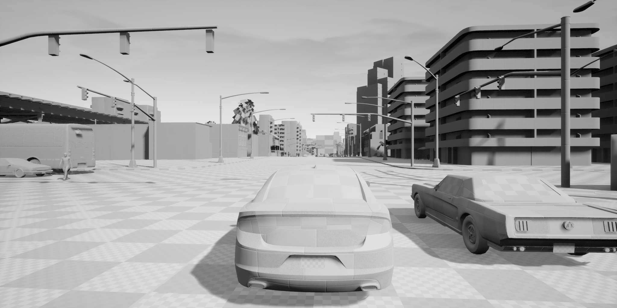
In the case of simulated data where access to the rendering engine is granted, a nearly texture-free environment can be generated. The open-source simulator CARLA [21] was employed to generate a virtual environment devoid of texture. We replaced all objects’ textures by a gray checkerboard, a default texture pattern in CARLA. In addition, weather conditions were set to ’clear noon’ to obtain a uniform appearance of the sky. Strongly subsampled video sequences were recorded from an ego perspective in gray scale. This procedure provides an additional way to obtain the cues S+V in CARLA.
Remaining Cue Combinations and Summary
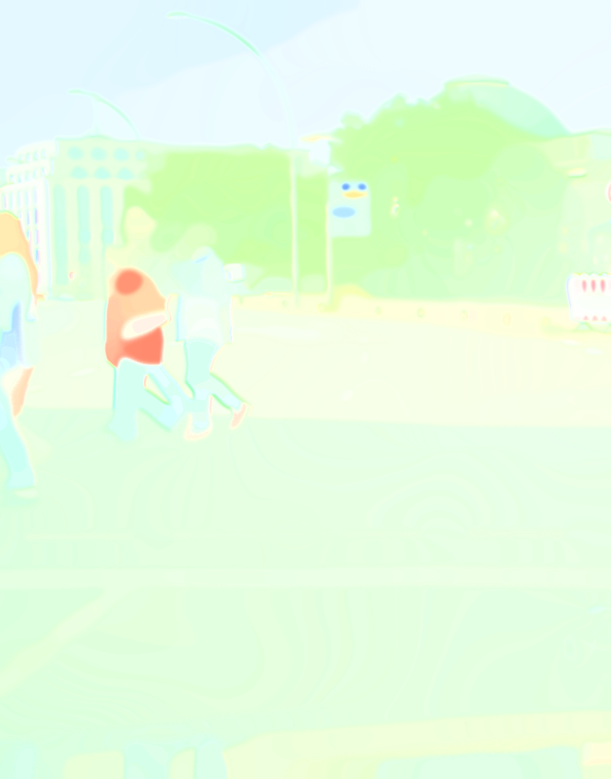
The remaining cue combinations are obtained as follows: S+T+V+HS, S+T+HS and S+T+V are obtained by treating an original image analogously to the color cue extraction, i.e., by transforming it into HSV color space and projecting accordingly. Analogously, we can process texture images to obtain T+HS as well as T+V. To represent the complete absence of cues, i.e. no information is given, we consider the performance of randomly initialized DNNs. An overview of all cue expert (datasets) including additional shorthands, encoding the method used and the cue extracted, are summarized in table I. Note that, in what follows we rely heavily on the shorthands. For additional technical details and exemplary images of the cue extraction methods, we refer the reader to sections A-A and A-B.
| shorthand | included cues | description | ||||||
|---|---|---|---|---|---|---|---|---|
| all cues | S | + | T | + | V | + | HS | original images / all cues |
| S | + | T | + | HS | all but gray cues | |||
| S | + | T | + | V | all but chromatic cues | |||
| T | + | V | + | HS | texture with color; shape removed | |||
| T | + | HS | texture with hue and saturation only | |||||
| T | + | V | texture with grayness only; | |||||
| S | + | V | + | HS | shape with color via smoothing texture by edge enhancing diffusion | |||
| S | + | HS | shape with hue and saturation by edge enhancing diffusion | |||||
| S | + | V | shape with grayness by grayscaled edge enhancing diffusion results | |||||
| S | shape only via contour map by holistically-nested edge detection | |||||||
| S | + | V | shape with grayness via texture removal in the CARLA simulation | |||||
| RGB | V | + | HS | complete color component of an RGB image, pixel-wise | ||||
| HS | HS | hue and saturation of an RGB image, pixel-wise | ||||||
| V | V | gray component of an RGB image, pixel-wise | ||||||
| no info | no information about the data is given representing the absence of all cues | |||||||
Late Fusion of Cue Experts
Fusing the cue experts’ softmax activations serves as an assessment of the reliability of the different cues to combine the information of multiple cues effectively.
IV Experiments
To analyze the cue influence in learning semantic segmentation tasks, we train all cue and cue combination experts on three different base datasets introduced below and ranging from real-world street scenes over synthetic street scenes to diverse in- and outdoor scenes. We perform an in-depth analysis and comparison of several cue (combination) experts across these three datasets, across different evaluation granularities ranging from dataset-level over class-level to pixel-level evaluations. This is complemented by a comparison of CNN and transformer results. Additional experimental studies and qualitative examples are provided in section A-C.
IV-A Base Datasets & Networks
Cityscapes
Cityscapes [19] is an automotive dataset which consists of high-resolution images of street scenes from (mostly German) cities with pixel annotations for classes, respectively. There are fine labeled training and validation images. As common practice we use only the common classes and the validation data for testing. For model selection purposes we created another validation set from a subset of the coarsely annotated images of Cityscapes by pseudo-labelling that subset using an off-the-shelf DeepLabV3+ [33].
CARLA
We generated a dataset using the open-source simulator CARLA [21], version 0.9.14, containing multiple enumerated maps of which we used the towns – and of similar visual detail level for data generation. We record one frame per second from an ego perspective while driving with autopilot through a chosen city, accumulating frames per city in total. For comparability to Cityscapes, we reduced the set of considered classes to : road, sidewalk, building, wall, pole, traffic lights, traffic sign, vegetation, terrain, sky, person, car, truck, bus, guard rail. The classes ‘bicycle’, ‘rider’ and ‘motorcycle’ are excluded for technical reasons because these actors were problematic for the autopilot mode in CARLA. To ensure a location-wise disjoint training and test split, we use town and for testing only, whereas and are used for training. This results in training images and test images. For model selection purposes, we randomly split of 10% of the training images for validation.
PASCAL Context
As a third dataset we analyze cue influences on the challenging PASCAL Context dataset [20]. It provides annotations for the whole images of PASCAL VOC 2010 [34] in semantic segmentation style. The images are photographs from the flickr111https://www.flickr.com photo-sharing website recorded and uploaded by consumers covering diverse indoor and outdoor scenes [34]. We consider labels that are contextual categories from [20]. In our experiments we use training images, validation images and test images where the training images of [20] are split into training and validation images and the original validation images are utilized as test images.
Neural Networks and Training Details
For better comparison and to ensure that only the intended cues are learned, all neural networks are trained from scratch multiple times with different random seeds. For all cue (combination) expert models, except for the color cue ones, we employ DeepLabV3 with a ResNet18 backbone [35, 36] ( million learnable parameters) and a SegFormer model with B1 backbone [37] ( million learnable parameters). Both models have similar learning capacity and achieve similar mean IoU (mIoU) [38] segmentation accuracy. For the color experts, the receptive field is constrained to one pixel, achieved through a fully convolutional neural network with two to three ()-convolutions (tuned to achieve maximal mIoU). We trained the CNN models with the Adam optimizer for epochs and a poly-linear learning rate decay with an initial learning rate of . The transformers were trained with the default optimizer and inference settings as specified in the MMSegmentation library [39] except that we increased the number of gradient update steps to iterations. Note that, to not mix cues unexpectedly, we restricted data augmentation to cropping and horizontal flipping and refrained from augmentations like color jittering. For the late-fusion approach, we use an even smaller version of DeepLabV3 by limiting the backbone to two instead of four blocks to prevent overfitting to the simpler task. The weights of the late fusion models are initialized randomly within a uniform distribution of .
IV-B Numerical Results
Cue Influence on Mean Segmentation Performance
In this section, we investigate the accuracies of the different cue (combination) experts in terms of mIoU when evaluated on the test base images across the three different base datasets. To ensure input compatibility, we evaluate experts with reduced channels like the V expert on the corresponding data. Comparing the performance drop (gap) between the reduced model and the full model demonstrates the significance of the removed cues in terms of their impact on the original semantic segmentation task. The corresponding results are presented in tables II and III. Firstly, we note a certain consistency in the presented mIoU results across base datasets. C experts are mostly dominated by T experts as well as S experts, and those are in turn dominated by S+T experts. The S+T+V expert is the only one getting close to the ‘expert’ trained on all cues. The order of the specific experts varies slightly across datasets, however not drastically. Also across all three datasets the RGB version of EED providing the cues S+C achieves surprisingly high mIoU values, indicating that in presence of color and shape, a DNN can learn well without having access to texture. However, this mIoU value is dominated by S+T+V as well as S+T+HS. Note that a combination of S+T only is impossible since T cannot exist without some kind of brightness or color cue, i.e., V and/or HS.
| Color | CNN mIoU | CNN gap | transformer mIoU | transformer gap | change in rank | ||||
| S | T | V | HS | (%, ) | (pp., ) | (%, ) | (pp., ) | w.r.t. CNN | |
| no info | |||||||||
| V | ✓ | ||||||||
| HS | ✓ | ||||||||
| RGB | ✓ | ✓ | |||||||
| ✓ | |||||||||
| ✓ | ✓ | ||||||||
| ✓ | ✓ | ||||||||
| ✓ | ✓ | ✓ | |||||||
| ✓ | ✓ | ||||||||
| ✓ | ✓ | ||||||||
| ✓ | ✓ | ✓ | |||||||
| ✓ | ✓ | ✓ | |||||||
| ✓ | ✓ | ✓ | |||||||
| all cues | ✓ | ✓ | ✓ | ✓ | |||||
| CARLA | PASCAL Context | ||||||
|---|---|---|---|---|---|---|---|
| mIoU | gap | rank change w.r.t. | mIoU | gap | rank change w.r.t. | ||
| () | (pp., ) | Cityscapes CNN | () | (pp., ) | Cityscapes CNN | ||
| no info | no info | ||||||
| V | V | ||||||
| HS | |||||||
| HS | |||||||
| RGB | RGB | ||||||
| all cues | |||||||
| all cues | |||||||
An additional surprise might be that HED, representing the S cue, reaches only very low mIoU, showing consistently weak performance across all datasets. At the first glance, this is in contrast to human vision since an HED image seems almost enough for a human to estimate the class of each segment in an HED image, cf. fig. 1. It should be noted that each expert is trained on its specific cue and then tested on an original input image from the given base dataset. When alternatively applying a given experts cue extraction technique as pre-processing to real-world images, like Cityscapes or PASCAL Context, HED (with HED pre-processing) surpasses EED (with EED-pre-processing) distinctly and achieves percent points (pp.) mIoU compared to pp. by EED on Cityscapes. On CARLA, EED and HED are on par, reaching an mIoU of pp. and pp. respectively.

Cue Influence on Different Semantic Classes
 |
 |
 |
Cityscapes |
 |
 |
 |
CARLA |
|
Context PASCAL |
|||
| expert | expert | ground truth |
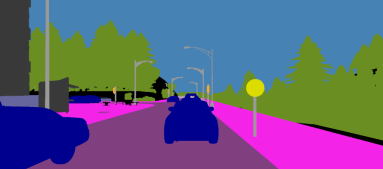
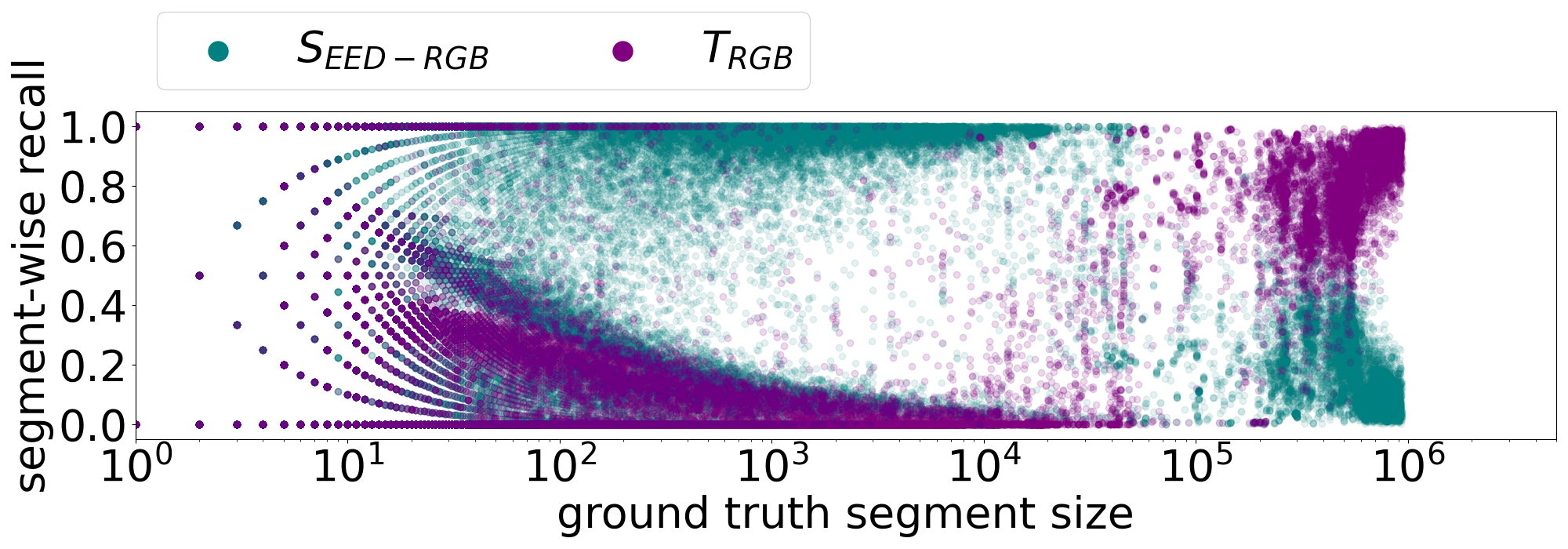
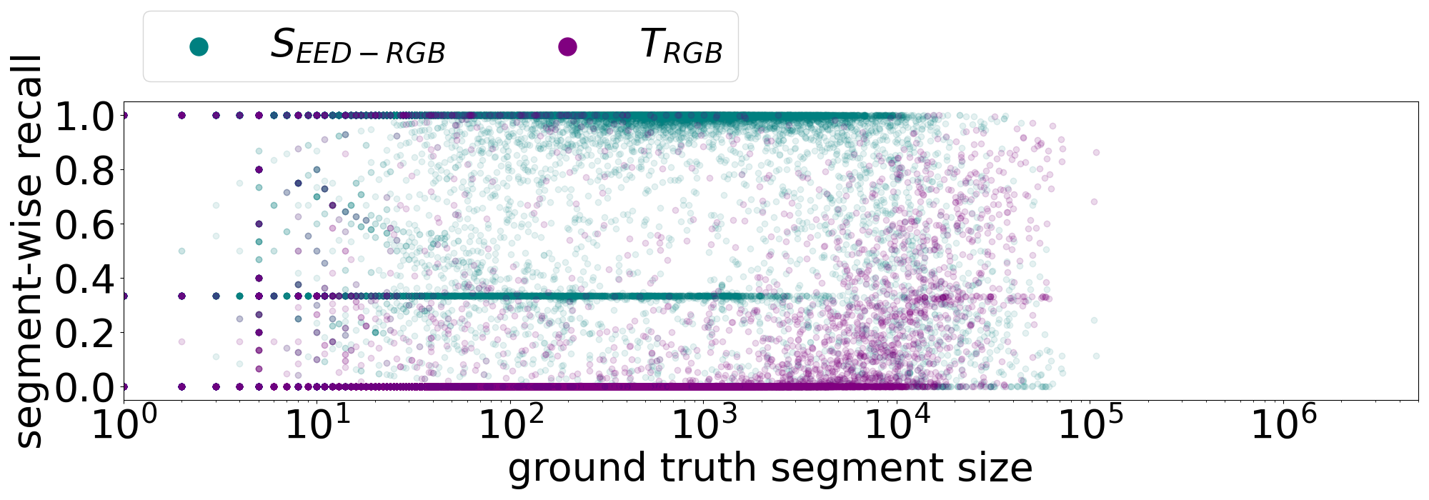
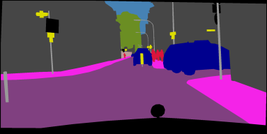
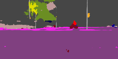
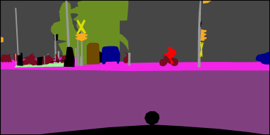
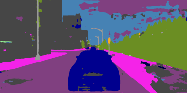
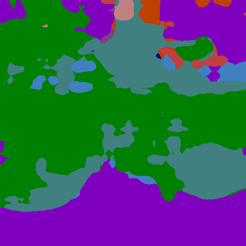
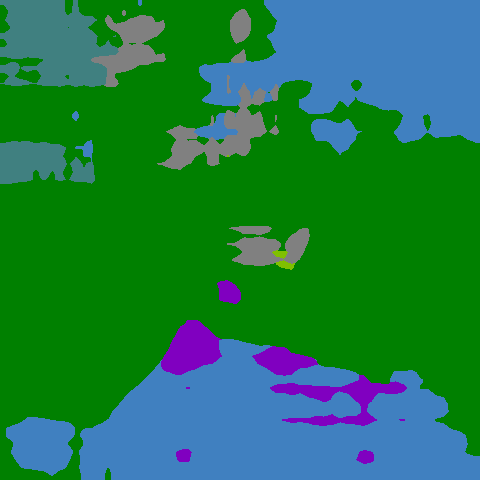
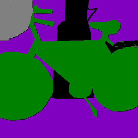
Figure 3 provides an evaluation for Cityscapes, comparing a shape expert based on colored EED images providing the cues S+C and another expert trained on colored Voronoi cells of class-specific stitched patches, providing the queues T+C. This evaluation is broken down into IoU values over the Cityscapes classes. In a visual inspection, we found that an IoU of at least for a given class starts to support the claim that the chosen expert extracts information for the given class. Hence, we see in fig. 3 that the S+C expert can deal with most of the classes while the T+C expert specializes to classes that usually cover large areas of the image, like vegetation, road and building, see also figs. 4 and 15 for visual examples. This size dependence is also studied in fig. 6 for CARLA as base dataset for the classes road and person, where the former contains large ground truth segments and the latter small ones. The quality of detection of a ground truth segment is measured in terms of a segment-wise recall, which is the fraction of pixels in the ground truth segment that are covered by a prediction of the same class. It can be seen that for the large road segments, the texture expert achieves a high segment-wise recall, indeed finding most of the road segments, while the shape expert has only a low segment-wise recall for those large segments.
Cue Influence Dependent on Location in an Image


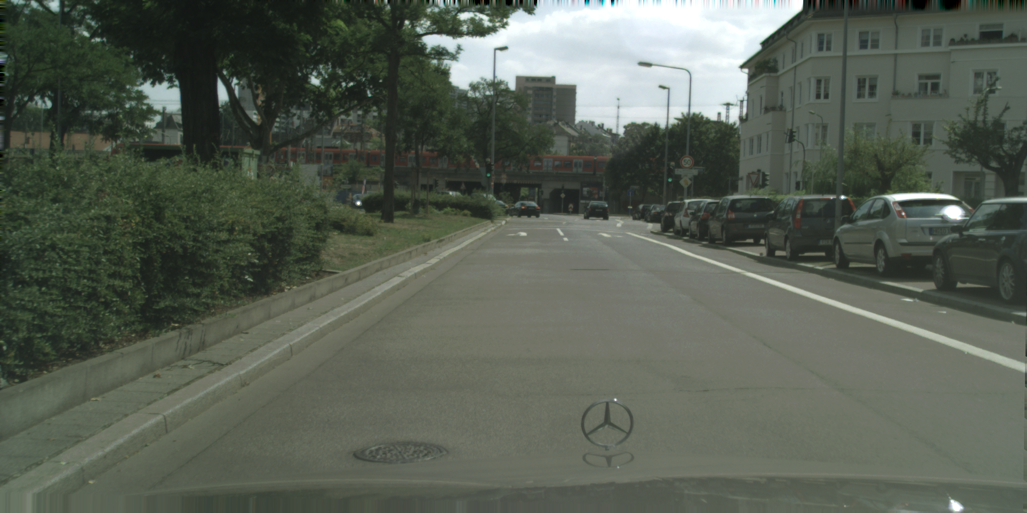

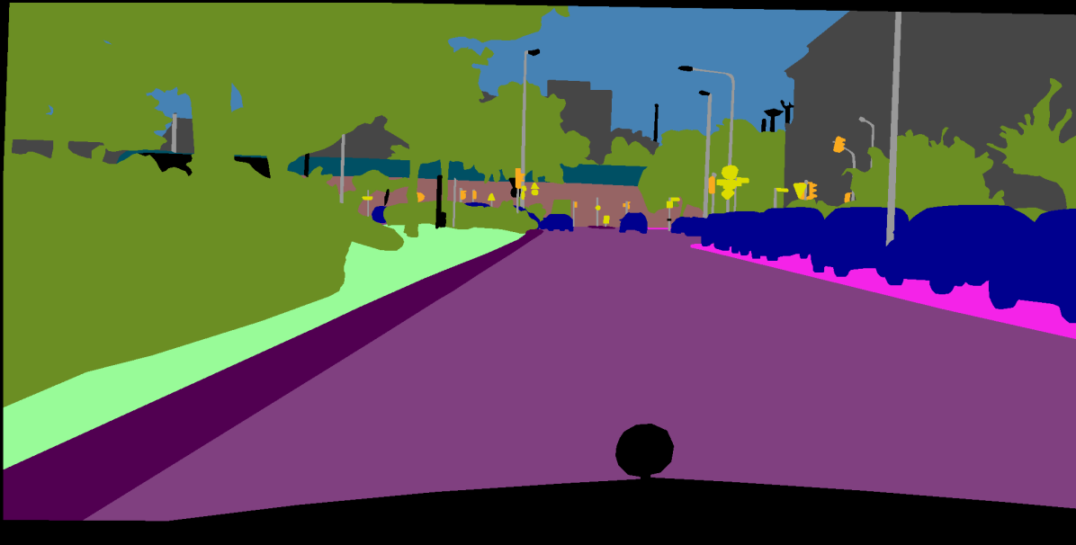
In this paragraph, we provide a detailed comparison of the same two experts from the previous paragraph, the shape expert based on EED having access to the cues S and C, and the texture expert based on the Voronoi images having access to the cues T and C. Here, cues are considered based on their location in an image, and we provide results for all three datasets.
We already noted in the previously presented class-specific study that the T+C expert focuses on classes covering larger areas of an image. To study this effect in-depth, we trained a late fusion that processes the softmax outputs of both experts T+C and S+C, learning a pixel-wise weighting of both expert’s outputs. A visual example for Cityscapes is provided in fig. 5. In general, we observed that the shape influences the fusion in regions containing boundaries of class-segments while priority is given to the texture inside larger segments. As can also be seen in fig. 5, the texture experts often have difficulties to accurately segment the boundaries of areas corresponding to a semantic class. We measured this effect quantitatively and provide results in table IV. The results reveal that the shape experts clearly outperform the texture expert on segment boundaries in terms of accuracy averaged over all boundary pixels. Herein, a pixel is considered as part of a segment boundary, if its neighborhood of four pixels distance (in Manhattan metric) contains a pixel of a different class according to the ground truth. On the segments’ interior, on Cityscapes and PASCAL Context, the shape expert is on average still more useful than the texture expert. This is the other way round in CARLA. This can be explained by the observations that Cityscapes is in general relatively poor in texture and the textures in both real-world datasets are not very discriminatory. However, in the driving simulator CARLA, the limited number of different textures rendered onto objects is highly discriminatory and increases the texture expert’s performance. Quantitative and additional qualitative results for the late fusion of cue experts are provided in the appendix.
| pixel-averaged | Cityscapes | CARLA | PASCAL Context | |||
|---|---|---|---|---|---|---|
| accuracy (%, ) | ||||||
| segment interior | ||||||
| segment boundary | ||||||
| overall | ||||||
Cue Influence in Different Architectures
In addition to the previously discussed CNN-based cue experts, we also studied the cue extraction capabilities of a segmentation transformer, namely SegFormer-B1 [37]. The results on Cityscapes are provided in table II. Although the CNN and transformer mIoU is almost on par when all cues are present, we observe a distinct increase in mIoU for the individual cue experts when using a transformer instead of a CNN. This holds for all T experts and S experts and their combinations with V and HS with one exception which is the HED cue extraction. We expect that the HED mIoU suffers from the strong domain shift between HED images and original images, to which the HED expert is applied in table II. Similarly, SegFormer achieves an mIoU of pp. when applying HED as pre-processing. Nonetheless, qualitatively, i.e., in terms of the rankings of the different cue experts, we do not observe any serious differences between CNNs and transformers. These findings generalize to the class level where we observe an increase in performance in nearly all classes independent of the expert, but qualitatively the influence of the cues does not change.
V Conclusion and Outlook
In this paper, we provided the first study on what can be learned by semantic segmentation DNNs from different image cues. Here, as opposed to image classification, studying cue influence is much more intricate and yields more specific and more fine-grained results. We introduced a generic procedure to extract cue-specific datasets from a given semantic segmentation dataset and studied several cue (combination) expert models, CNNs and transformers, across three different datasets and different evaluation granularities. We compared different cue (combination) experts in terms of mIoU on the whole dataset, in terms of semantic classes and in terms of image-location dependence. Except for grayscale images, there is no reduced cue combination that achieves a performance close to all cues. Cues influence the learning of DNNs over image locations, indeed shape often matters more in the vicinity of semantic class boundaries. Shape cues are important for all classes, texture cues mostly for classes where the corresponding segment covers large regions of the images in the dataset. We expect that our generic cue extraction procedure (or at least parts of it) can also be utilized for studying biases in pre-trained off-the-shelf DNNs in cue conflict schemes, typical for that field of research.
Acknowledgments
This work is supported by the German Federal Ministry for Economic Affairs and Climate Action within the project “KI Delta Learning”, grant no. 19A19013Q. We thank the consortium for the successful cooperation. A. M., N. G., E. H. and M. R. acknowledge support through the junior research group project “UnrEAL” by the German Federal Ministry of Education and Research (BMBF), grant no. 01IS22069. Moreover, the authors gratefully acknowledge the Gauss Centre for Supercomputing e.V. (www.gauss-centre.eu) for funding this project by providing computing time through the John von Neumann Institute for Computing (NIC) on the GCS Supercomputer JUWELS at [40] (JSC).
References
- [1] Robert A. Jacobs “What Determines Visual Cue Reliability?” In Trends in Cognitive Sciences 6.8 Elsevier, 2002, pp. 345–350 DOI: 10.1016/S1364-6613(02)01948-4
- [2] Kaitlyn R. Bankieris, Vikranth Rao Bejjanki and Richard N. Aslin “Sensory Cue-Combination in the Context of Newly Learned Categories” In Scientific Reports 7.1 Nature Publishing Group, 2017, pp. 10890 DOI: 10.1038/s41598-017-11341-7
- [3] Melchi M. Michel and Robert A. Jacobs “Learning Optimal Integration of Arbitrary Features in a Perceptual Discrimination Task” In Journal of Vision 8.2, 2008, pp. 3 DOI: 10.1167/8.2.3
- [4] Robert Geirhos et al. “ImageNet-trained CNNs Are Biased towards Texture; Increasing Shape Bias Improves Accuracy and Robustness” In International Conference on Learning Representations, 2018
- [5] Md Amirul Islam et al. “Shape or Texture: Understanding Discriminative Features in CNNs” In International Conference on Learning Representations, 2021
- [6] Shikhar Tuli, Ishita Dasgupta, Erin Grant and Thomas L. Griffiths “Are Convolutional Neural Networks or Transformers More like Human Vision?” arXiv, 2021 arXiv:2105.07197 [cs]
- [7] Jonas Kubilius, Stefania Bracci and Hans P. Beeck “Deep Neural Networks as a Computational Model for Human Shape Sensitivity” In PLOS Computational Biology 12.4 Public Library of Science, 2016, pp. e1004896 DOI: 10.1371/journal.pcbi.1004896
- [8] Nicholas Baker, Hongjing Lu, Gennady Erlikhman and Philip J. Kellman “Deep Convolutional Networks Do Not Classify Based on Global Object Shape” In PLOS Computational Biology 14.12 Public Library of Science, 2018, pp. e1006613 DOI: 10.1371/journal.pcbi.1006613
- [9] Hossein Hosseini, Baicen Xiao, Mayoore Jaiswal and Radha Poovendran “Assessing Shape Bias Property of Convolutional Neural Networks” In arXiv:1803.07739, 2018 arXiv:1803.07739
- [10] Jia Deng et al. “ImageNet: A Large-Scale Hierarchical Image Database” In IEEE Conference on Computer Vision and Pattern Recognition, 2009, pp. 248–255 DOI: 10.1109/CVPR.2009.5206848
- [11] Wieland Brendel and Matthias Bethge “Approximating CNNs with Bag-of-local-Features Models Works Surprisingly Well on ImageNet” In International Conference on Learning Representations, 2018
- [12] Paul Gavrikov et al. “Are Vision Language Models Texture or Shape Biased and Can We Steer Them?” In arXiv:2403.09193, 2024 arXiv:2403.09193
- [13] Christoph Kamann and Carsten Rother “Increasing the Robustness of Semantic Segmentation Models with Painting-by-Numbers” In Computer Vision – ECCV 2020, Lecture Notes in Computer Science Cham: Springer International Publishing, 2020, pp. 369–387 DOI: 10.1007/978-3-030-58607-2˙22
- [14] Muhammad Muzammal Naseer et al. “Intriguing Properties of Vision Transformers” In Advances in Neural Information Processing Systems 34 Curran Associates, Inc., 2021, pp. 23296–23308
- [15] Xinkuan Qiu et al. “Shape-biased CNNs are Not Always Superior in Out-of-Distribution Robustness” In Proceedings of the IEEE/CVF Winter Conference on Applications of Computer Vision, 2024, pp. 2326–2335
- [16] Yingwei Li et al. “Shape-Texture Debiased Neural Network Training” In International Conference on Learning Representations, 2020
- [17] Dawei Dai et al. “Rethinking the Image Feature Biases Exhibited by Deep Convolutional Neural Network Models in Image Recognition” In CAAI Transactions on Intelligence Technology 7.4, 2022, pp. 721–731 DOI: 10.1049/cit2.12097
- [18] Katherine Hermann, Ting Chen and Simon Kornblith “The Origins and Prevalence of Texture Bias in Convolutional Neural Networks” In Advances in Neural Information Processing Systems 33 Curran Associates, Inc., 2020, pp. 19000–19015
- [19] Marius Cordts et al. “The Cityscapes Dataset for Semantic Urban Scene Understanding” In Proceedings of the IEEE Conference on Computer Vision and Pattern Recognition, 2016, pp. 3213–3223
- [20] Roozbeh Mottaghi et al. “The Role of Context for Object Detection and Semantic Segmentation in the Wild” In IEEE Conference on Computer Vision and Pattern Recognition (CVPR), 2014
- [21] Alexey Dosovitskiy et al. “CARLA: An Open Urban Driving Simulator” In Conference on Robot Learning PMLR, 2017, pp. 1–16
- [22] Robert Geirhos et al. “Unintended cue learning: Lessons for deep learning from experimental psychology” In Journal of Vision 20.11 The Association for Research in VisionOphthalmology, 2020, pp. 652–652
- [23] Aditay Tripathi, Rishubh Singh, Anirban Chakraborty and Pradeep Shenoy “Edges to Shapes to Concepts: Adversarial Augmentation for Robust Vision” In Proceedings of the IEEE/CVF Conference on Computer Vision and Pattern Recognition, 2023, pp. 24470–24479
- [24] Robert Geirhos et al. “Partial Success in Closing the Gap between Human and Machine Vision” In Advances in Neural Information Processing Systems 34 Curran Associates, Inc., 2021, pp. 23885–23899
- [25] Johannes Theodoridis, Jessica Hofmann, Johannes Maucher and Andreas Schilling “Trapped in Texture Bias? A Large Scale Comparison of Deep Instance Segmentation” In Computer Vision – ECCV 2022, Lecture Notes in Computer Science Cham: Springer Nature Switzerland, 2022, pp. 609–627 DOI: 10.1007/978-3-031-20074-8˙35
- [26] Yixin Zhang and Maciej A. Mazurowski “Convolutional Neural Networks Rarely Learn Shape for Semantic Segmentation” In Pattern Recognition 146, 2024, pp. 110018 DOI: 10.1016/j.patcog.2023.110018
- [27] Chaithanya Kumar Mummadi et al. “Does Enhanced Shape Bias Improve Neural Network Robustness to Common Corruptions?” In International Conference on Learning Representations, 2020
- [28] Edgar Heinert, Matthias Rottmann, Kira Maag and Karsten Kahl “Reducing Texture Bias of Deep Neural Networks via Edge Enhancing Diffusion” In arXiv:2402.09530, 2024 arXiv:2402.09530
- [29] Tiange Luo et al. “Defective Convolutional Networks” In arXiv:1911.08432, 2020 arXiv:1911.08432
- [30] Melissa Cote, Amanda Dash and Alexandra Branzan Albu “Semantic Segmentation of Textured Mosaics” In EURASIP Journal on Image and Video Processing 2023.1 SpringerOpen, 2023, pp. 1–26 DOI: 10.1186/s13640-023-00613-0
- [31] Jacob Feldman “Visual Perception: On the Trail of High-Level Shape Aftereffects” In Current Biology 34.5 Elsevier, 2024, pp. R195–R197 DOI: 10.1016/j.cub.2024.01.009
- [32] Saining Xie and Zhuowen Tu “Holistically-Nested Edge Detection” In Proceedings of IEEE International Conference on Computer Vision, 2015
- [33] Liang-Chieh Chen et al. “Encoder-Decoder with Atrous Separable Convolution for Semantic Image Segmentation” In Computer Vision – ECCV 2018, Lecture Notes in Computer Science Cham: Springer International Publishing, 2018, pp. 801–818 DOI: 10.1007/978-3-030-01234-2˙49
- [34] Mark Everingham et al. “The Pascal Visual Object Classes (VOC) Challenge” In International Journal of Computer Vision 88.2, 2010, pp. 303–338 DOI: 10.1007/s11263-009-0275-4
- [35] Liang-Chieh Chen, George Papandreou, Florian Schroff and Hartwig Adam “Rethinking Atrous Convolution for Semantic Image Segmentation” In arXiv:1706.05587, 2017 arXiv:1706.05587
- [36] Kaiming He, Xiangyu Zhang, Shaoqing Ren and Jian Sun “Deep Residual Learning for Image Recognition” In Proceedings of the IEEE Conference on Computer Vision and Pattern Recognition, 2016, pp. 770–778
- [37] Enze Xie et al. “SegFormer: Simple and Efficient Design for Semantic Segmentation with Transformers” In Advances in Neural Information Processing Systems, 2021
- [38] Paul Jaccard “The Distribution of the Flora in the Alpine Zone” In New Phytologist 11.2, 1912, pp. 37–50 DOI: 10.1111/j.1469-8137.1912.tb05611.x
- [39] MMSegmentation Contributors “OpenMMLab Semantic Segmentation Toolbox and Benchmark”, https://github.com/open-mmlab/mmsegmentation, 2020
- [40] Jülich Supercomputing Centre “JUWELS: Modular Tier-0/1 Supercomputer at the Jülich Supercomputing Centre” In Journal of large-scale research facilities 5.A135, 2019 DOI: 10.17815/jlsrf-5-171
- [41] Satoshi Suzuki and Keiichi Abe “Topological Structural Analysis of Digitized Binary Images by Border Following” In Computer Vision, Graphics, and Image Processing 30.1, 1985, pp. 32–46 DOI: 10.1016/0734-189X(85)90016-7
- [42] Salvatore Torquato “Cell and Random-Field Models” In Random Heterogeneous Materials: Microstructure and Macroscopic Properties, Interdisciplinary Applied Mathematics New York, NY: Springer, 2002, pp. 188–209 DOI: 10.1007/978-1-4757-6355-3˙8
- [43] Sivan Harary et al. “Unsupervised Domain Generalization by Learning a Bridge Across Domains” In Proceedings of the IEEE/CVF Conference on Computer Vision and Pattern Recognition, 2022, pp. 5280–5290
- [44] Simon Niklaus “A Reimplementation of HED Using PyTorch”, https://github.com/sniklaus/pytorch-hed, 2018
- [45] Pietro Perona, Takahiro Shiota and Jitendra Malik “Anisotropic diffusion” In Geometry-driven diffusion in computer vision Springer, 1994, pp. 73–92
- [46] Joachim Weickert “Anisotropic diffusion in image processing” Teubner Stuttgart, 1998
- [47] Joachim Weickert “Coherence-enhancing diffusion filtering” In International journal of computer vision 31 Springer, 1999, pp. 111–127
- [48] Joachim Weickert and Martin Welk “Tensor field interpolation with PDEs” In Visualization and processing of tensor fields Springer, 2006, pp. 315–325
- [49] Joachim Weickert, Martin Welk and Marco Wickert “L2-stable nonstandard finite differences for anisotropic diffusion” In Scale Space and Variational Methods in Computer Vision: 4th International Conference, SSVM 2013, Schloss Seggau, Leibnitz, Austria, June 2-6, 2013. Proceedings 4, 2013, pp. 380–391 Springer
Appendix A Appendix
In the appendix, we provide additional results as well as technical details of the procedure.
A-A Cue Decomposition
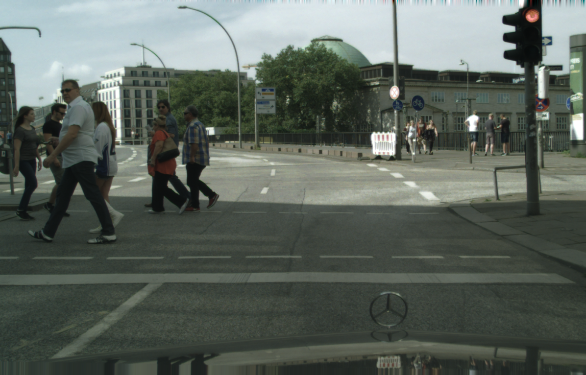
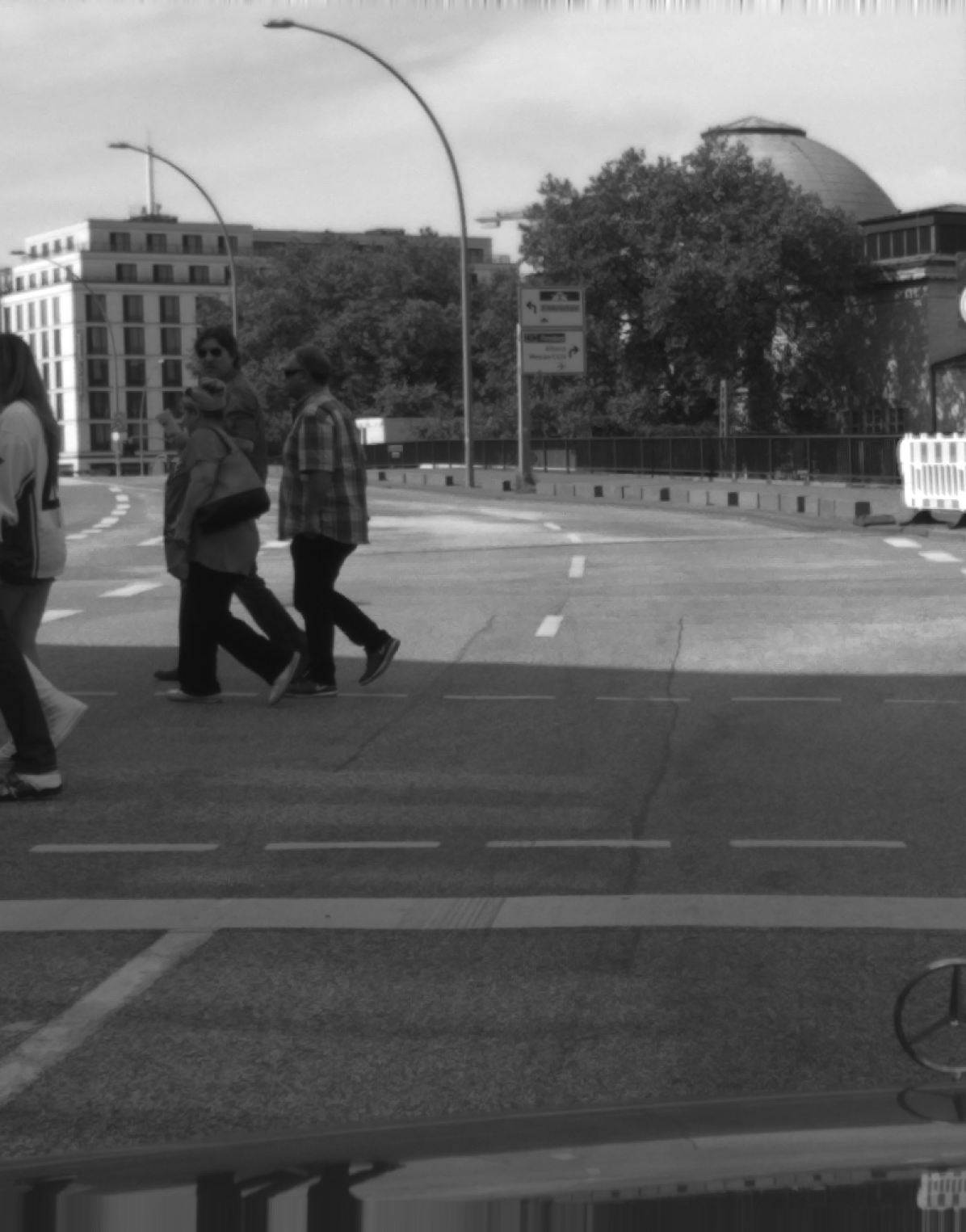
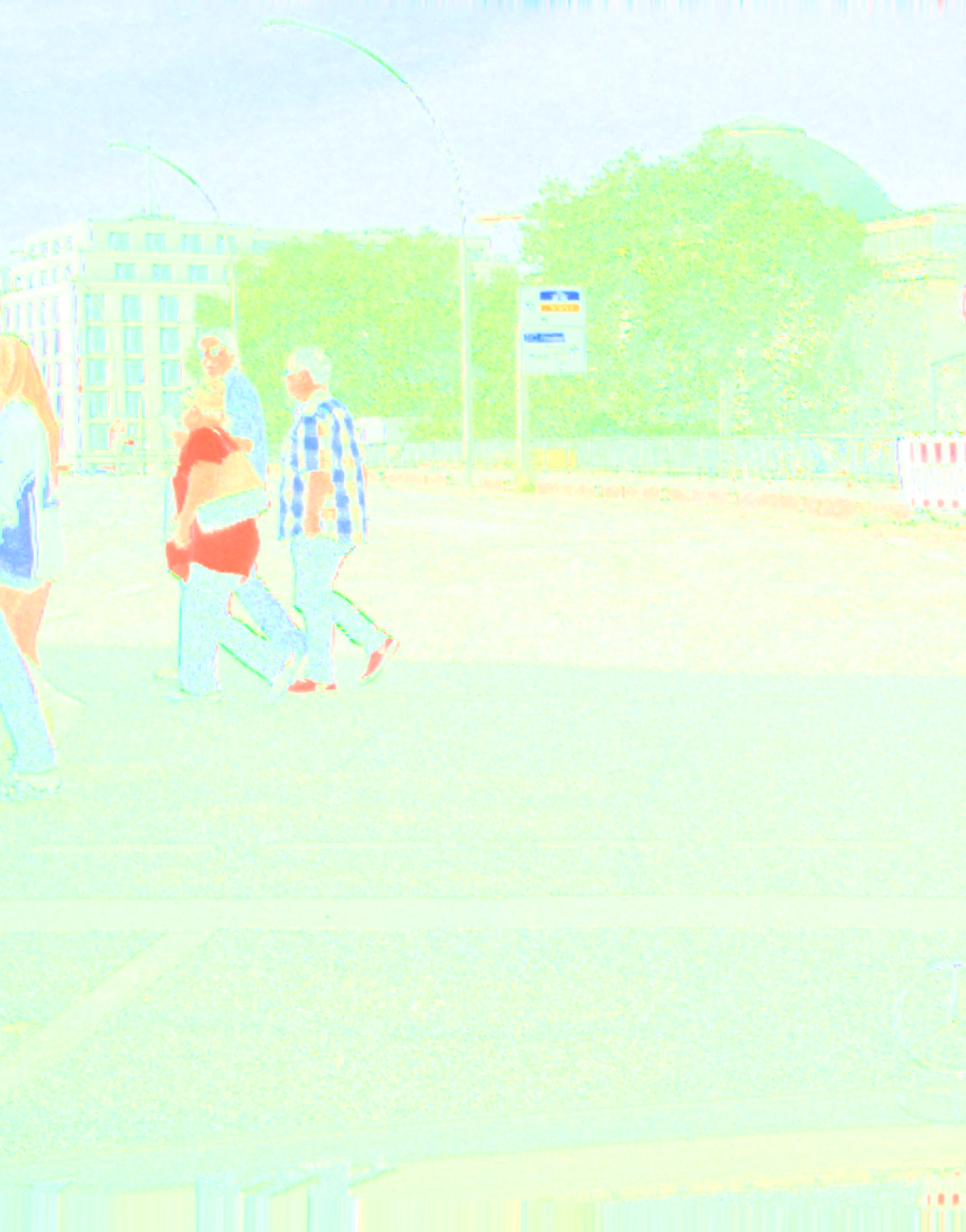
In fig. 7 we show exemplary images of cues extracted from the Cityscapes dataset. For all but the images containing the T cue, the cues can be extracted solely based on the base image (all cues). In contrast, the texture image is generated based on multiple images of the base dataset.
 (a) all cues
 (b)
(b)
 (c)
(c)
 (d)
(d)
 (e) T
(e) T
 (f)
(f)
 (g)
(g)
 (h)
(h)
 (i)
(i)
 (j) RGB
 (k)
(k)
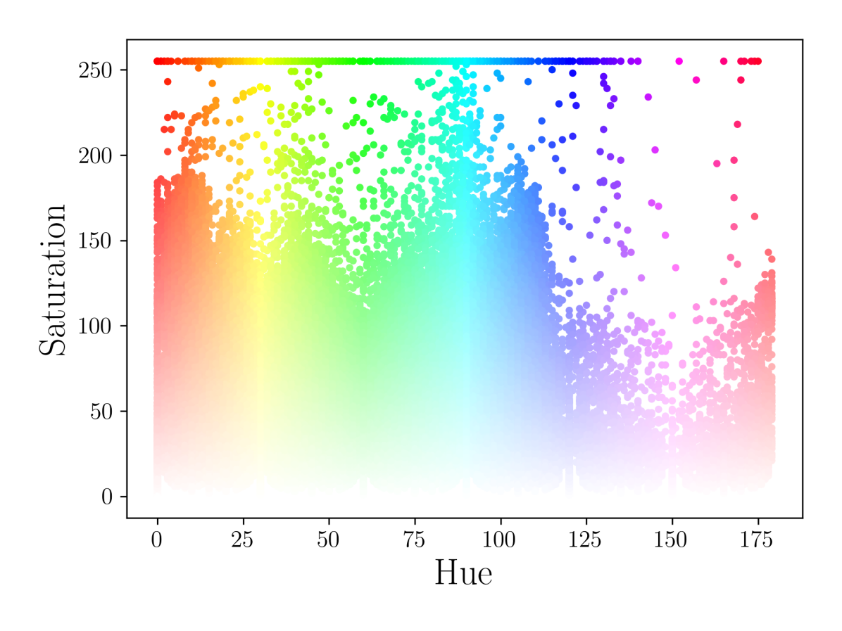 (l) HS
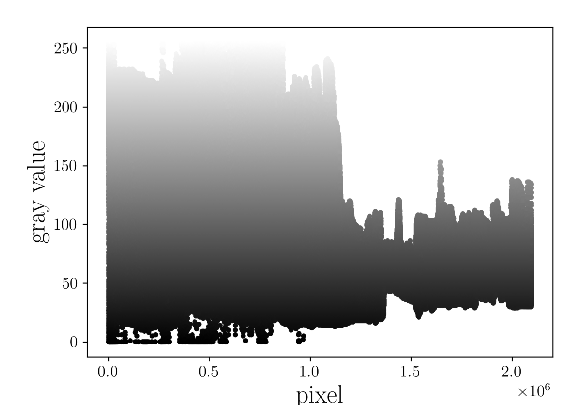 (m) gray
A-B Technical and Implementation Details
Texture Data Generation Details
A detailed scheme of the texture extraction procedure is given in fig. 8. The class-wise texture extraction is realized by masking all segments of one class and isolating each segment with the help of the border following algorithm proposed by [41]. We discard segments with less than pixels. The remaining segments are used to mask the original image and cut out the image patch of the enclosing bounding box of the segment. To enlarge the resulting patch pool, we apply horizontal flipping, random center crop and shift-scale-rotation augmentation. To mitigate the class imbalance in terms of pixel counts, we add more transformed patches for underrepresented classes than for classes which cover large areas of an image. It is essential to ensure that the transformations do not alter the texture. Once all the texture patches within the underlying dataset have been extracted, they are randomly composed into mosaic images. We iteratively fill images of the same size as images from the base dataset with overlapping texture patches until we obtain completely filled mosaic images. To further reduce an unintended dependency on the shape cue we fill the mosaics in the original segmentation mask but assign each pixel to the same class (contour filled texture images). This implies that the segment boundaries are not discriminatory anymore. Based on a pool of contour filled texture images of different classes we can create a surrogate segmentation task by filling the segments of arbitrary segmentation masks with the generated texture images. We choose Voronoi diagrams [42] as surrogate segmentation task and fill each cell randomly but uniformly with respect to the class with crops of the pool of contour filled texture images. To generate an entire dataset, we create and fill as many Voronoi diagrams as the number of images in the base dataset.
HED Implementation Details
EED Data Generation Details
EED is an anisotropic diffusion technique based on Partial Differential Equations (PDEs) [45, 46]. Starting with the original image as the initial value, it utilizes a spatially dependent variation of the Laplace operator to propagate color information along edges but not across them, thus leading to texture being largely removed from images and higher level features being largely preserved. For the production of the EED data [46] we have used a variation proposed in [28] that avoids circular artifacts and preserves shapes particularly well by applying spatial orientation smoothing as proposed for Coherence Enhancing Diffusion in [47]. The PDE is solved using explicit Euler, channel coupling from [48, p. 321] and the discretization described in [49, p. 380-391].
The diffusion parameters are the same for all three data sets, Cityscapes, CARLA and PASCAL Context:
-
•
Contrast parameter .
-
•
Gaussian blurring kernel size and standard deviation .
-
•
Time step length and artificial spatial distance .
-
•
Number of time steps .
-
•
Discretization parameters and .
For a visual example see fig. 7. The used implementation can be found in https://github.com/eheinert/reducing-texture-bias-of-dnns-via-eed/.
Carla Data Generation Details
Although CARLA claims to support online texture switching as of version 0.9.14, this feature is limited to specific instances and found to be inadequate for the purposes of this study. As a consequence, we manually modified each material instance, replacing surface textures with a basic default texture pattern (gray checkerboard). Since the sky is not a meshed object, it was not possible to manipulate its texture. Instead, we set the weather conditions to clear noon to achieve a uniform texture. The dataset is recorded by a vehicle in CARLA with an RGB camera and semantic segmentation sensor in the ego perspective driving in autopilot mode as described in section IV-A. In a post-processing step the images are gray scaled to remove the sky color. The basic components of the procedure are visualized in fig. 9.
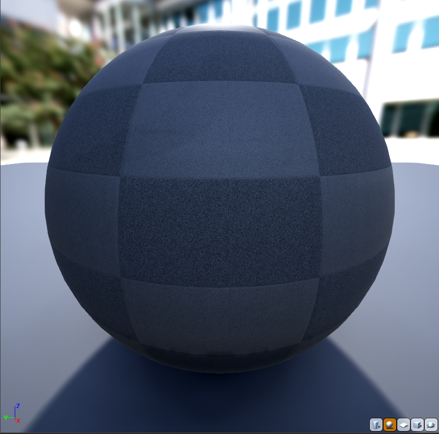
Model Implementation Details
For the CNN-based models we adapt the DeepLabV3 model from torchvision222https://github.com/pytorch/vision/blob/main/torchvision/models/segmentation/deeplabv3.py to our needs. For the transformer models we use the MMSegmentation framework [39].
A-C Additional Numerical Experiments
Comparison of Cue Influence Without Domain Shift
Except for the texture extraction procedure all cue extraction methods can be applied as an online transformation during inference. This allows us to compare the cue influence without domain shift for the shape experts. We observe that the S cue based on object contours () mostly outperforms other experts trained on shape cues, also when the latter receive additional color cue information, see table V.
| Cityscapes in-domain | CARLA in-domain | PASCAL Context in-domain | |
| mIoU (%, ) | mIoU (%, ) | mIoU (%, ) | |
| - | - |
Cue Influence on Different Semantic Classes
Figures 10, 11 and 12 show that the results reported on Cityscapes generalize to the other base datasets as well as to the transformer model. However, for the CARLA base dataset we observe that the texture is more discriminatory compared to the real-world datasets (cf. column ‘rank change’ in table III) and the performance of the expert on classes like road, sidewalk and building surpasses the performance of the comparable shape expert . In fig. 15 we provide additional qualitative results for this finding.


Cue Influence Dependent on Location in an Image
Furthermore, our analysis on pixel level reveals for the CARLA base dataset, that the S+C and T+C cues are complementary. Fusing and improves the overall scene understanding by a notable margin. The fusion model achieves a performance of mIoU on the CARLA test set which is about pp. superior to the test set performance of and more than pp. superior to when relying only on (cf. fig. 10). In CARLA the described dominated shape influence on segment boundaries (cf. table IV) is more pronounced and thus exploited by the fusion model, see fig. 13. Additional qualitative results of the fusion prediction and the corresponding pixel-wise weighting of the expert influence is depicted in fig. 14.
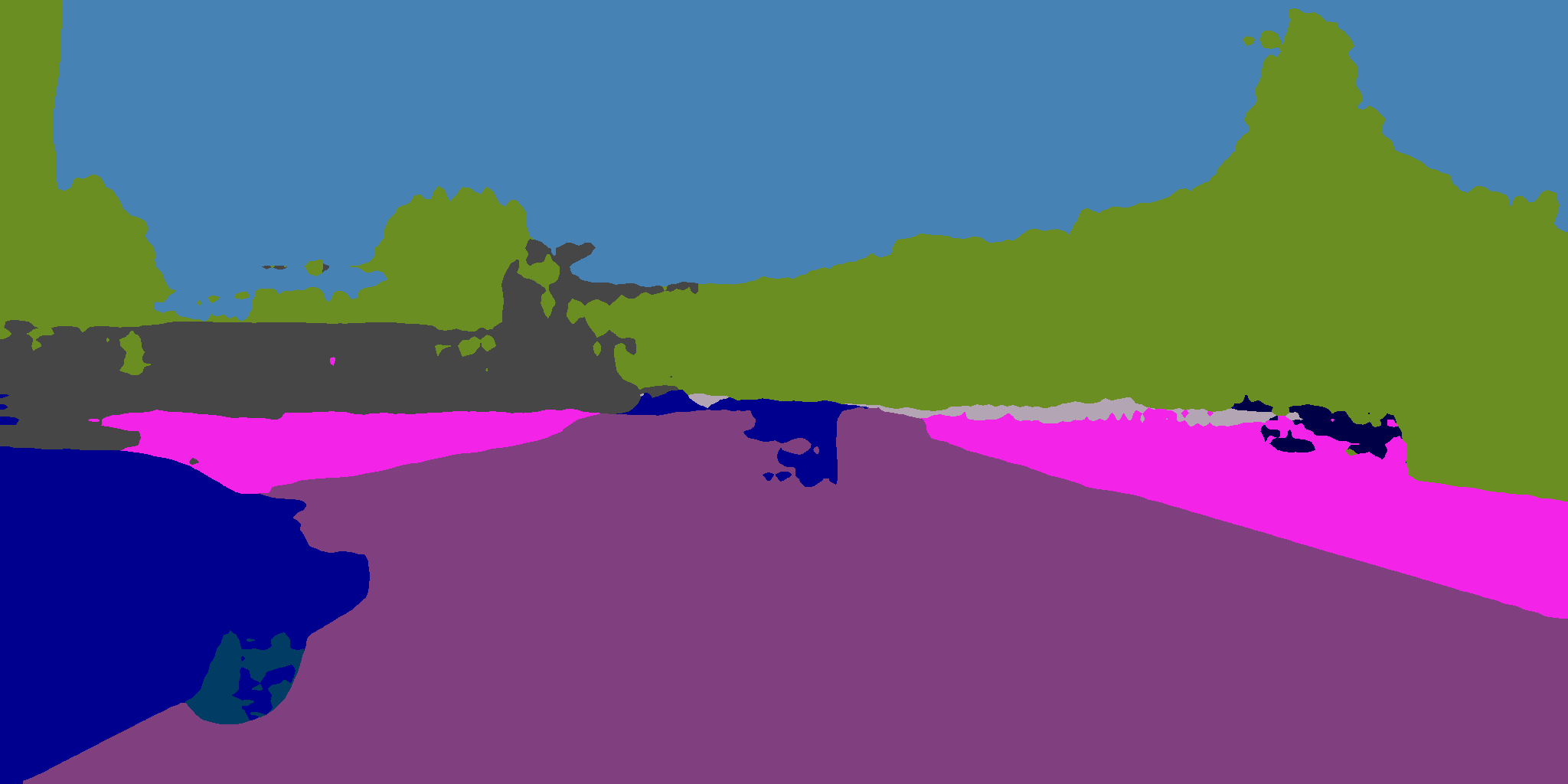
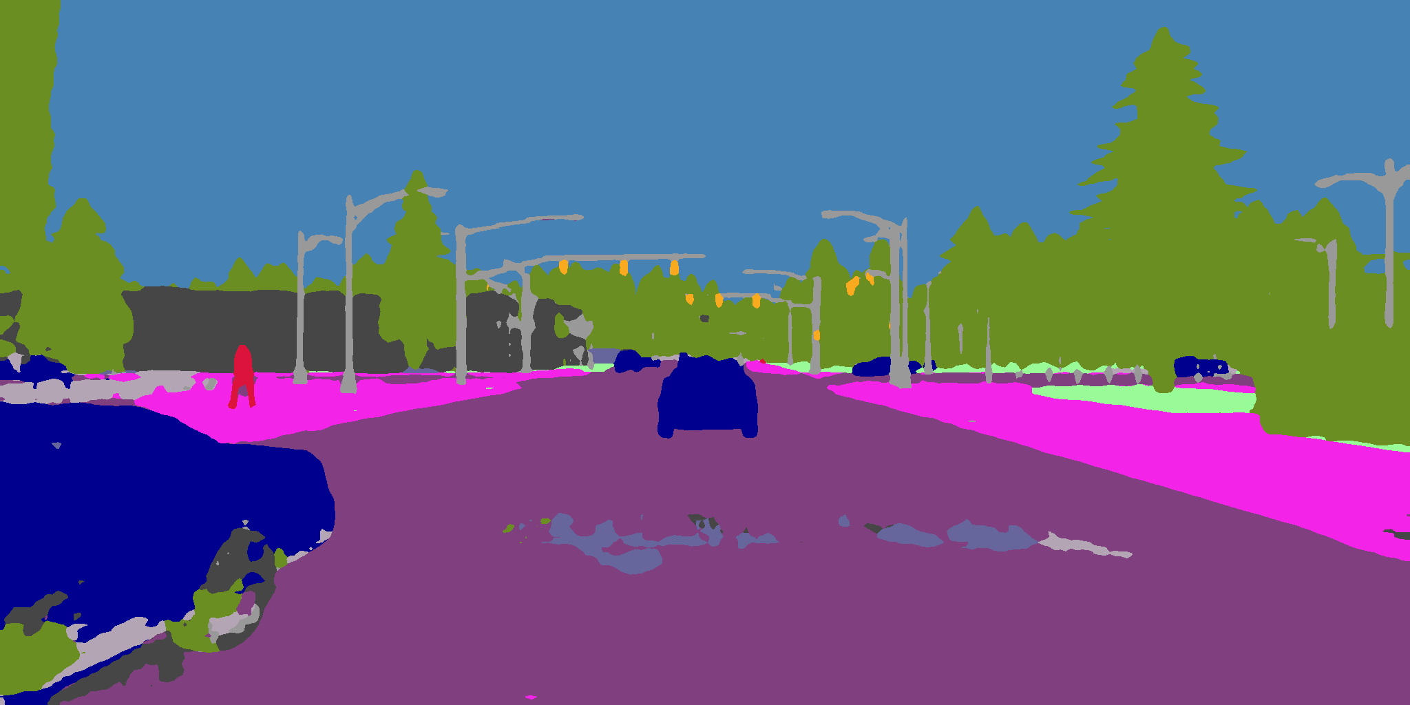
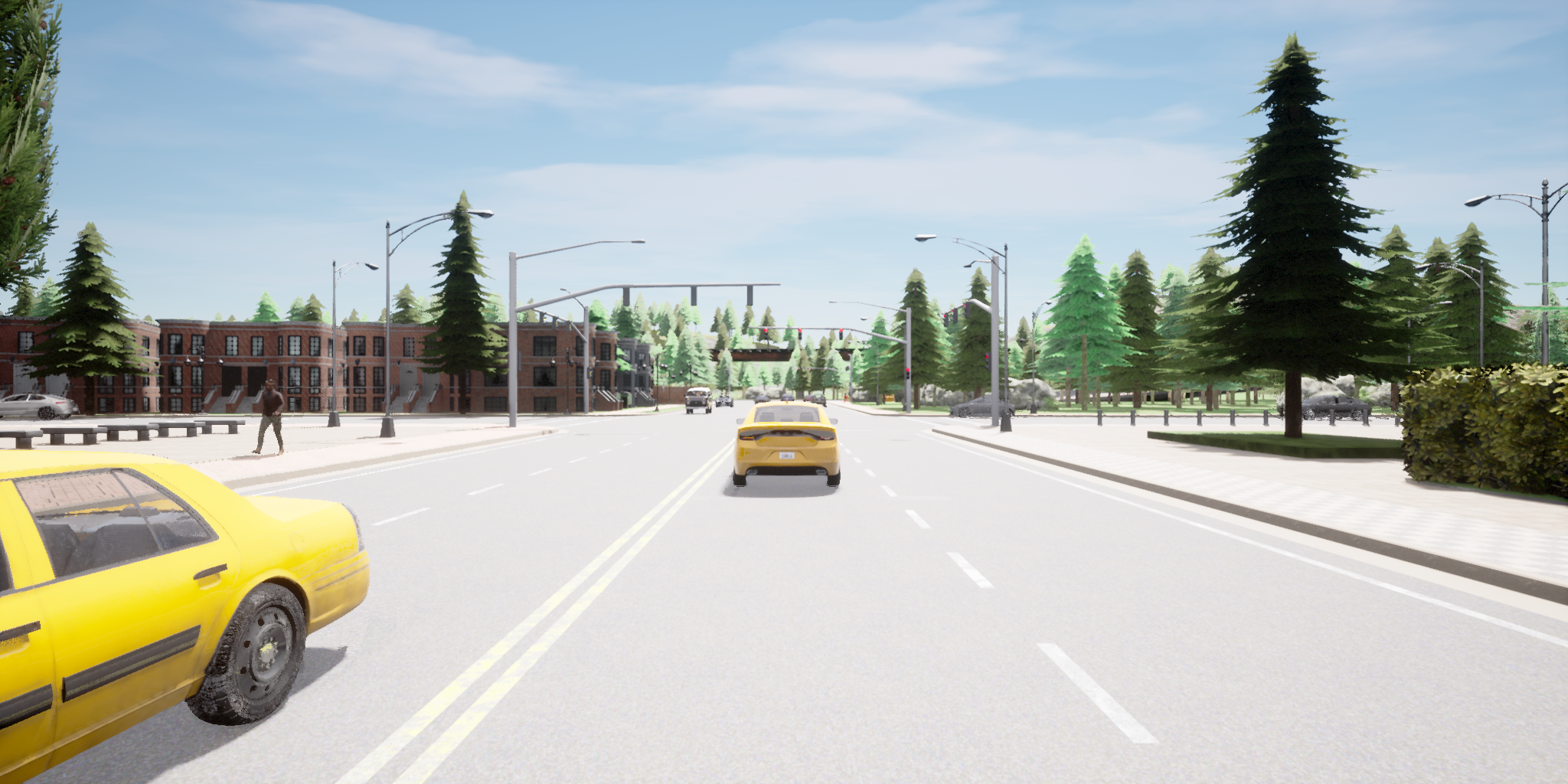
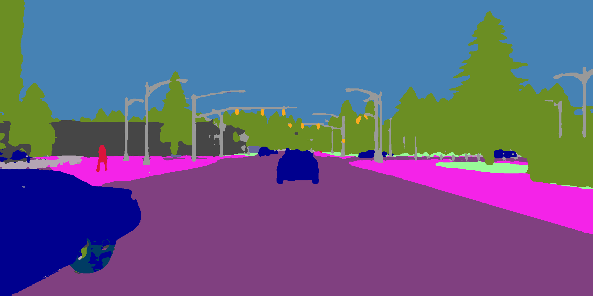
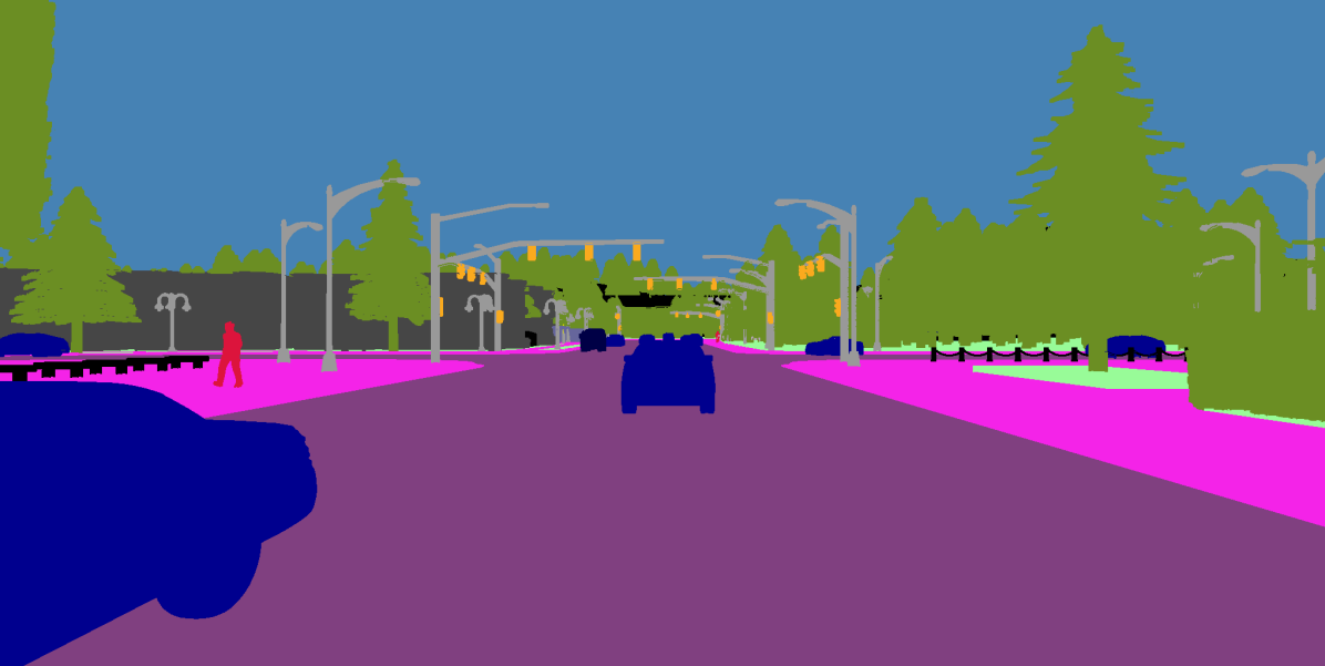
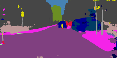
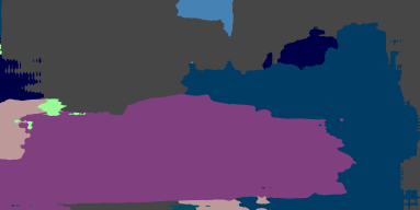
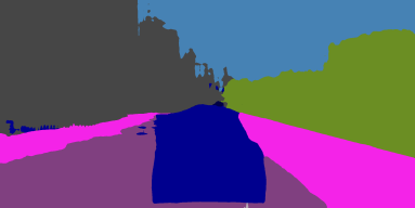
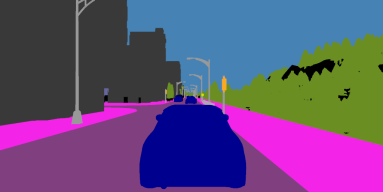
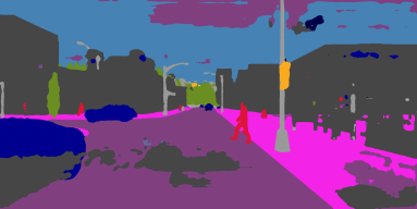
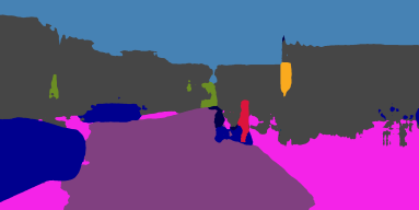
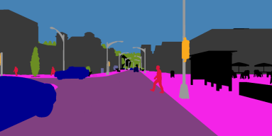
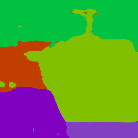
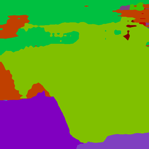
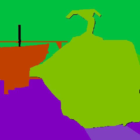
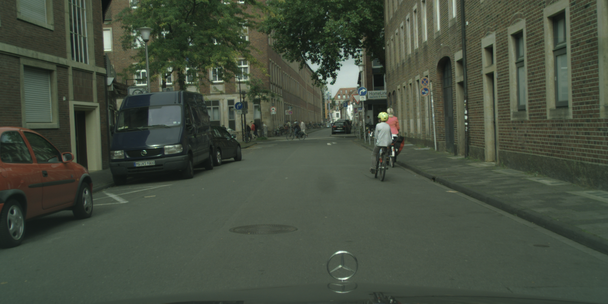
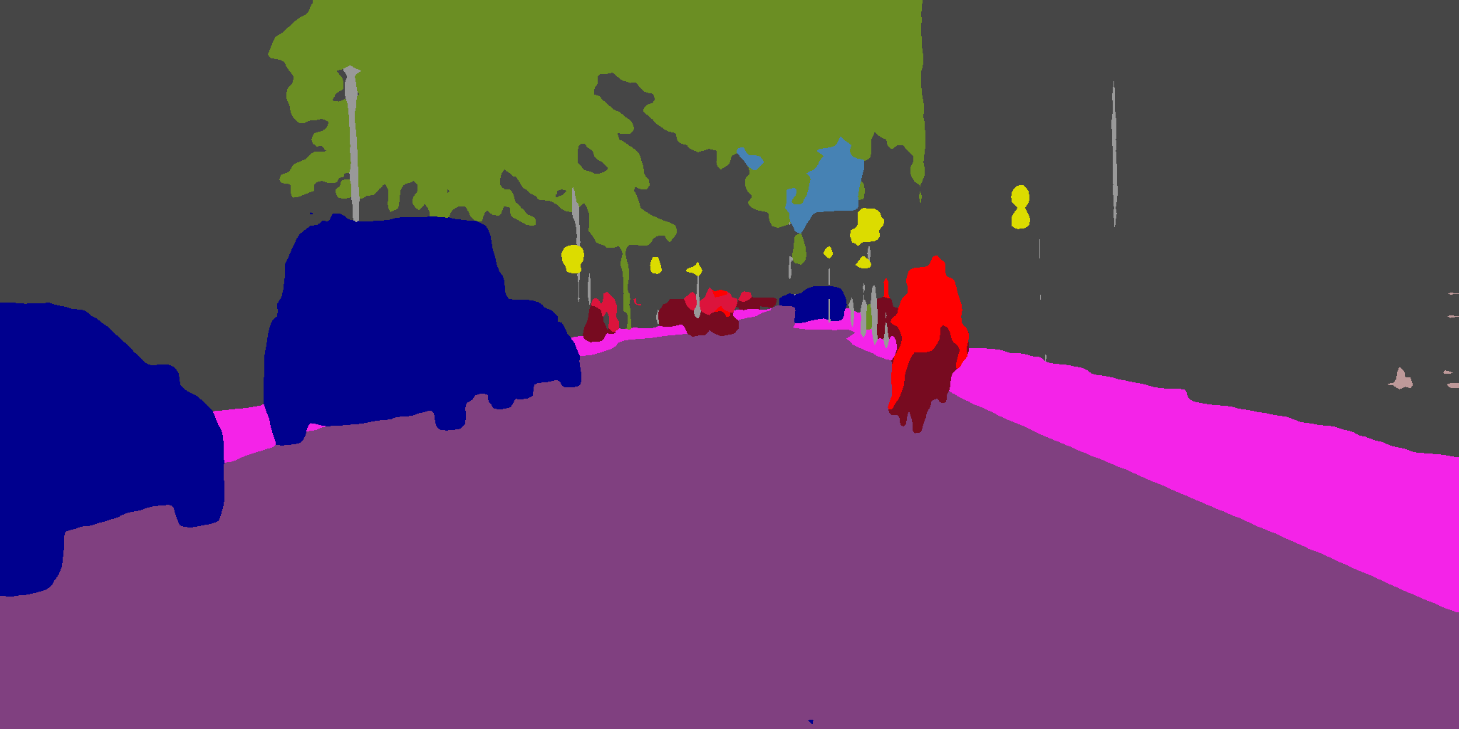
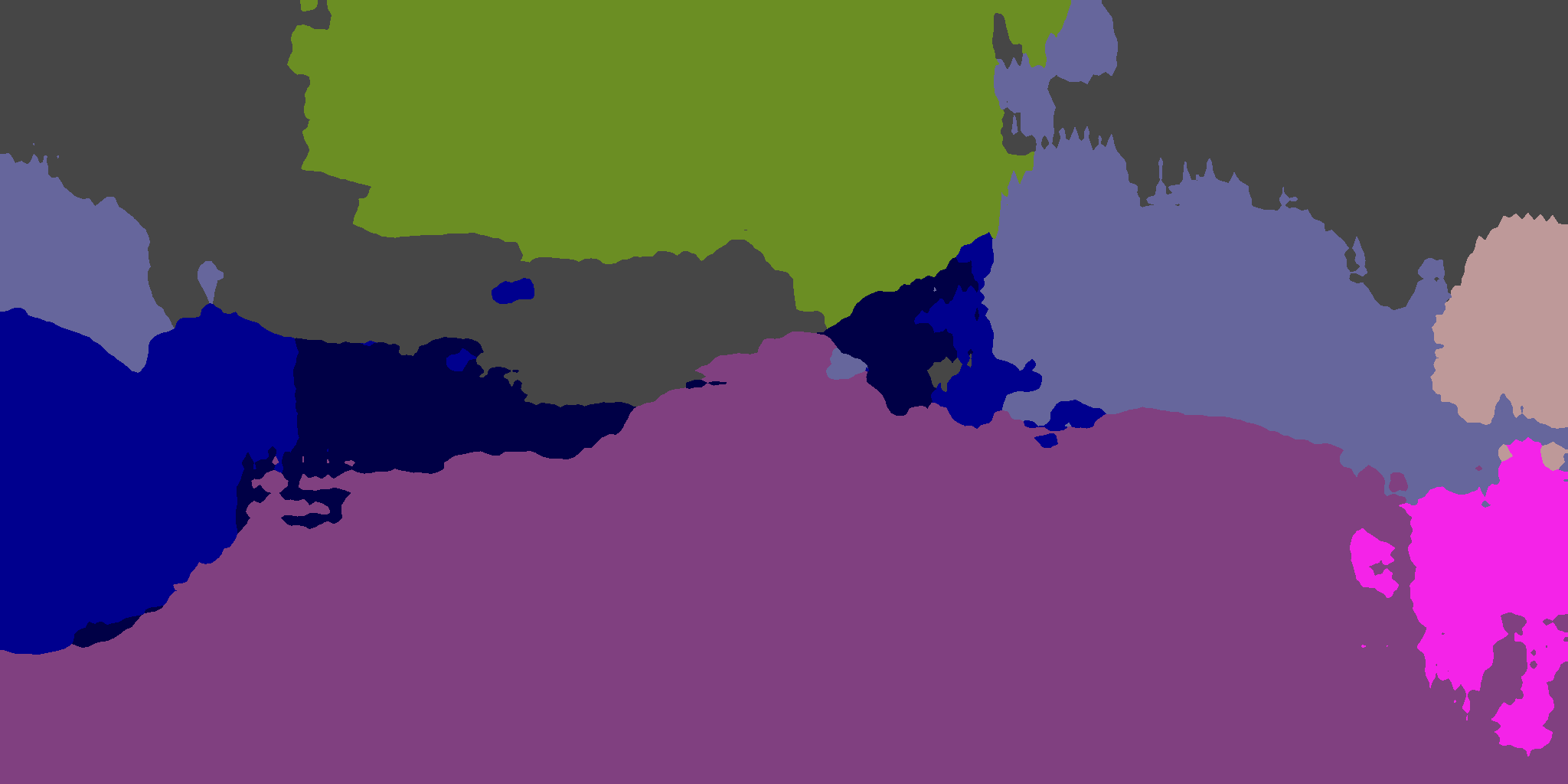
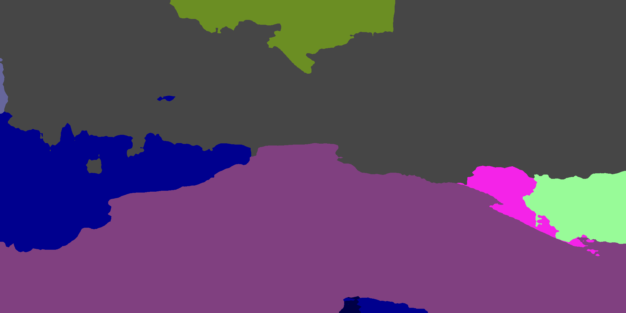
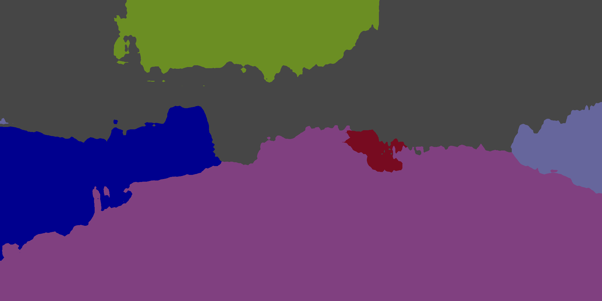
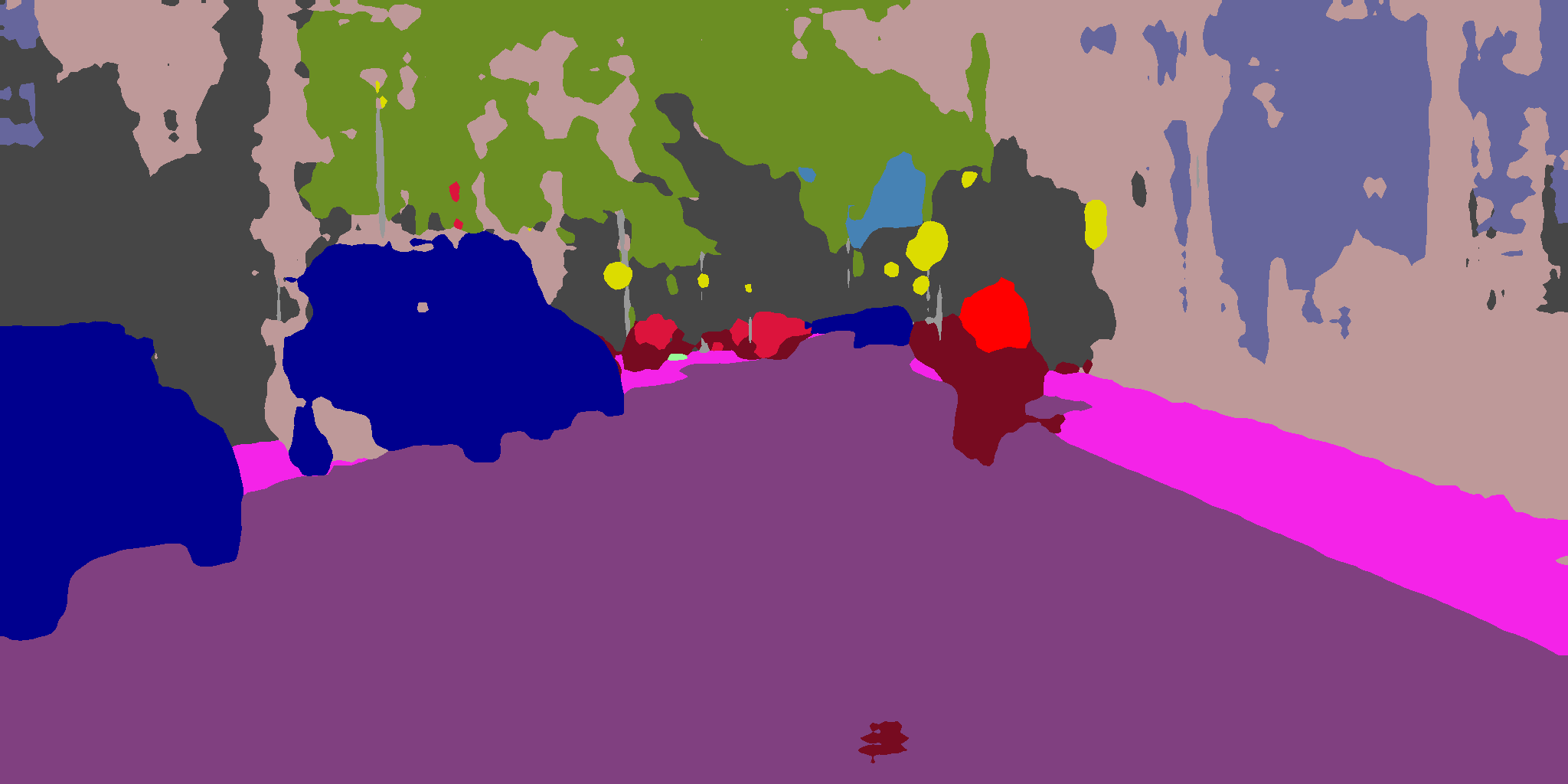
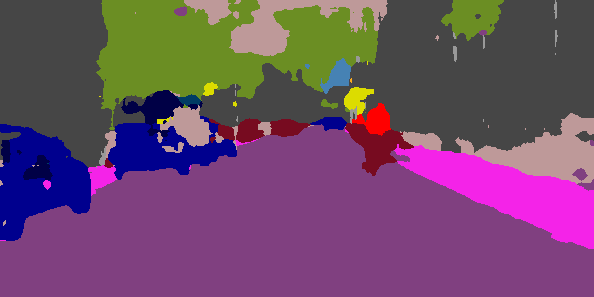
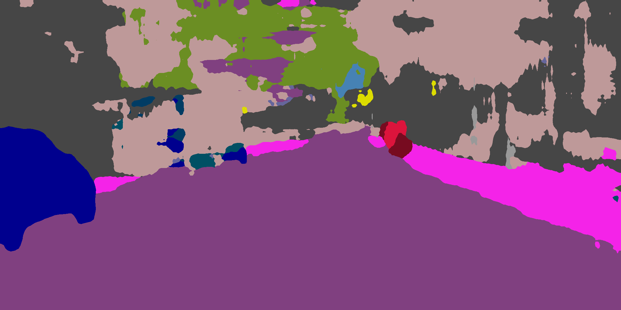
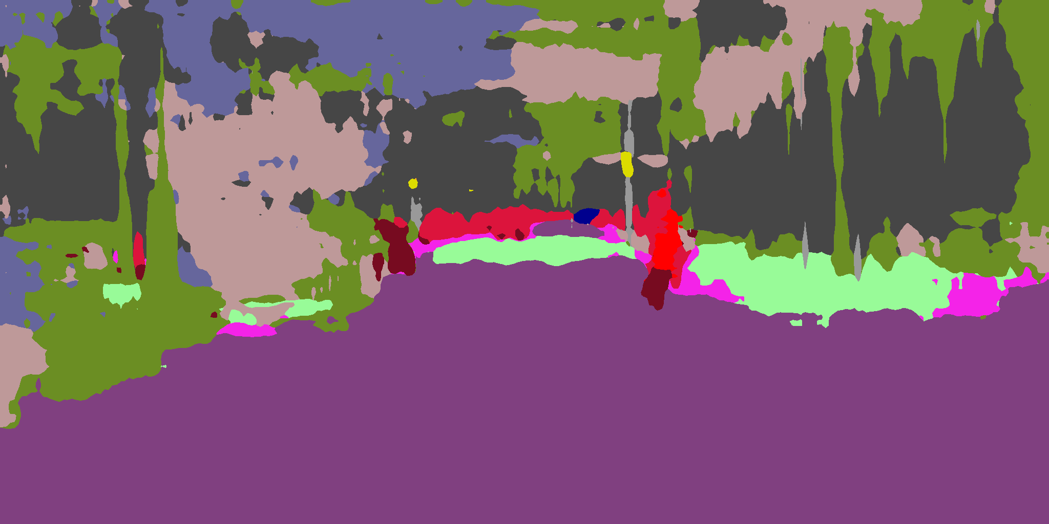
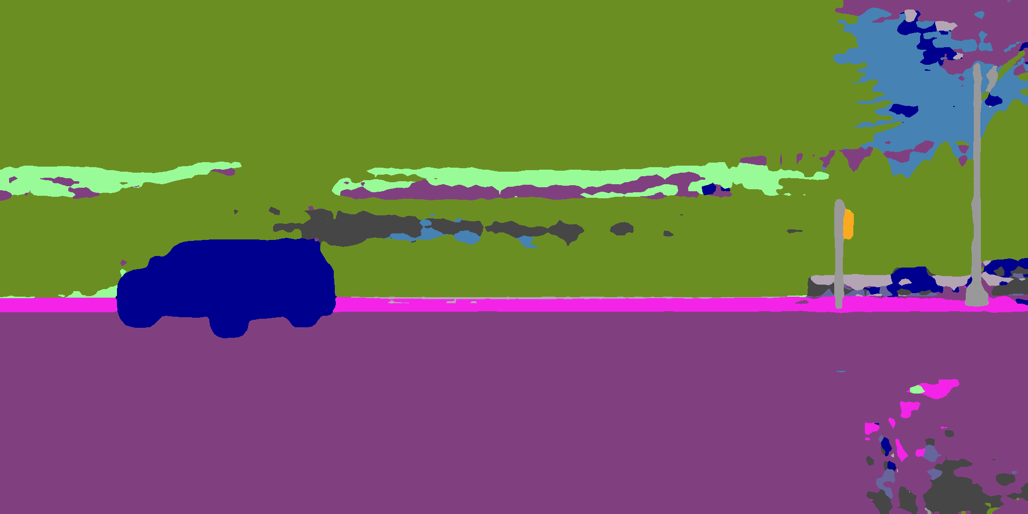
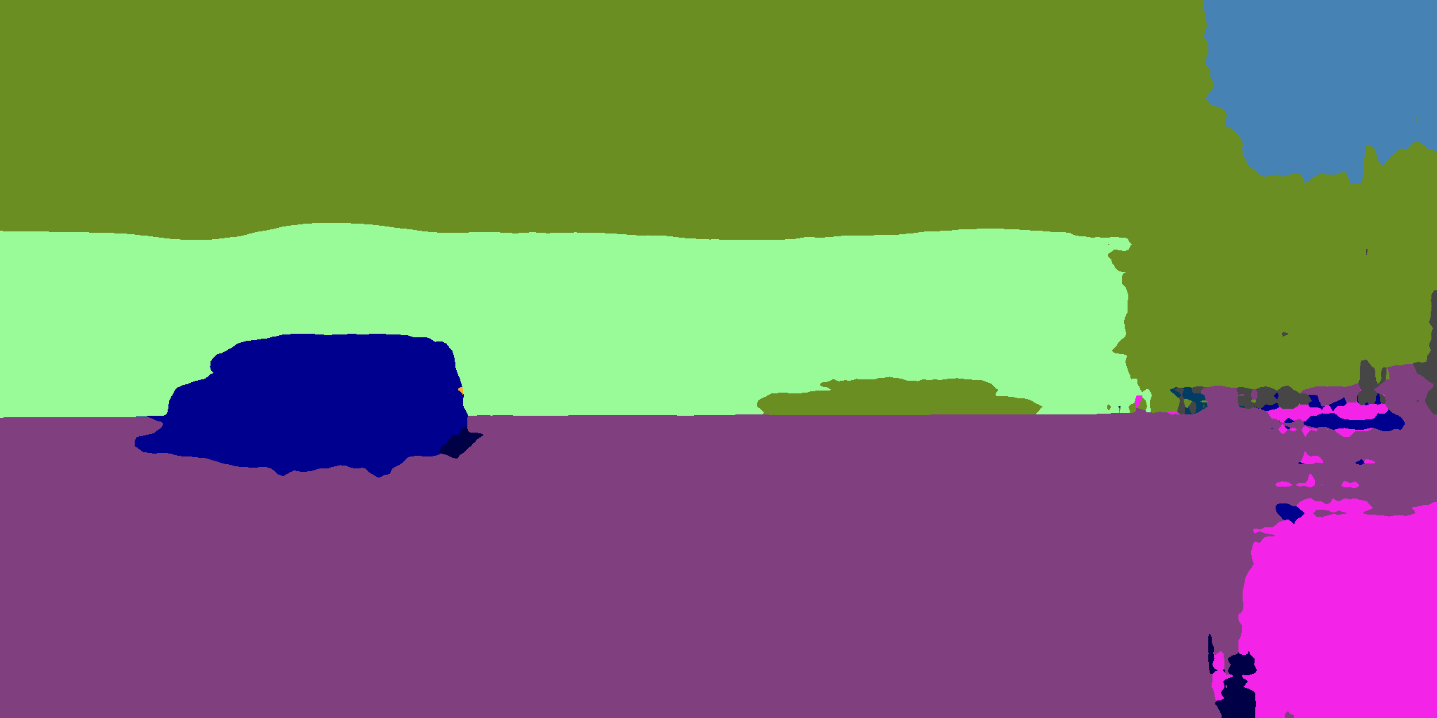
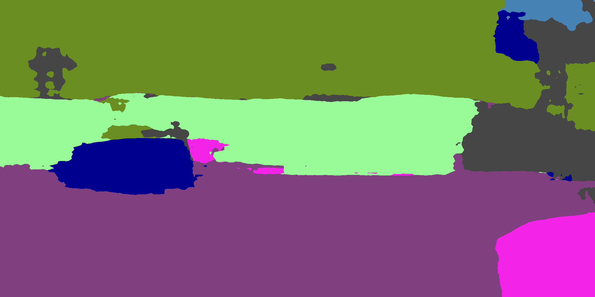
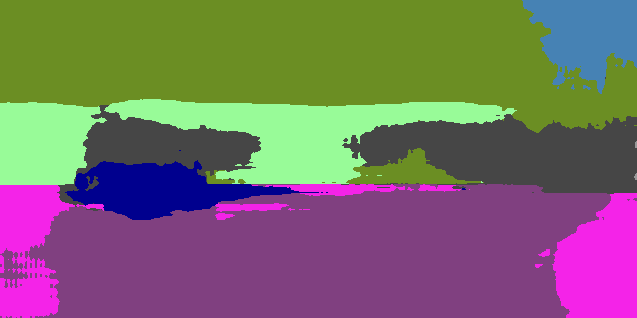
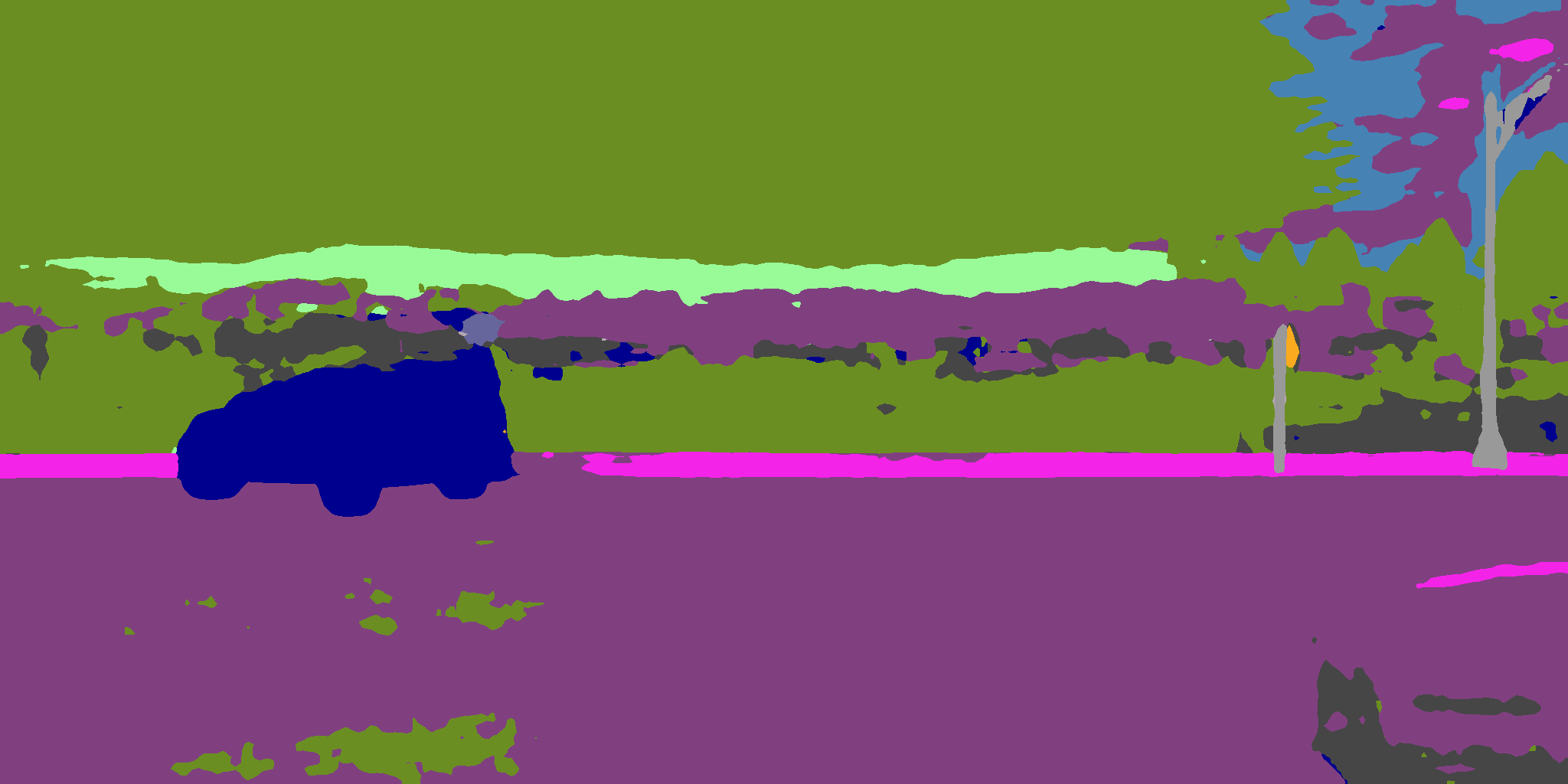
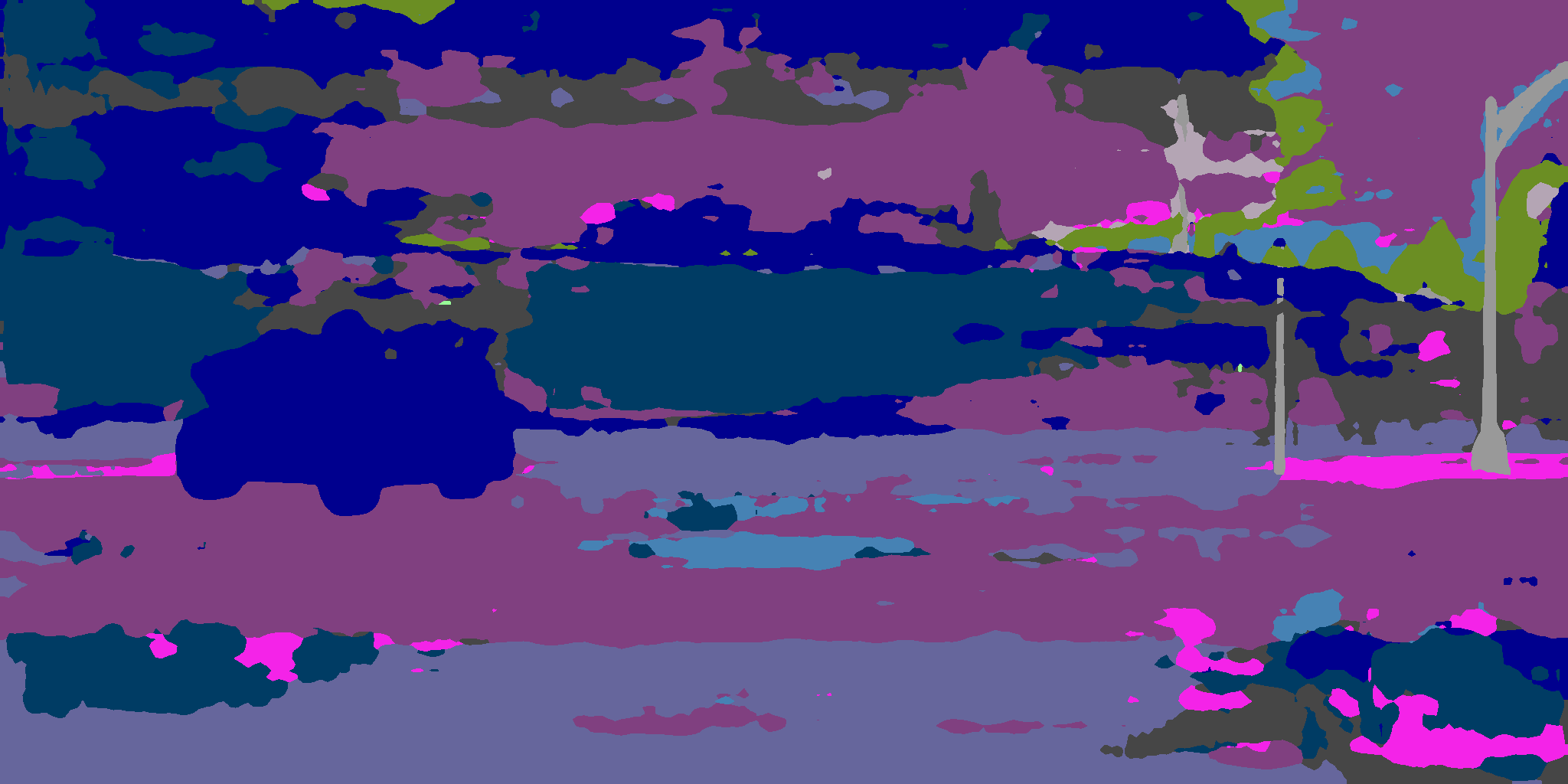
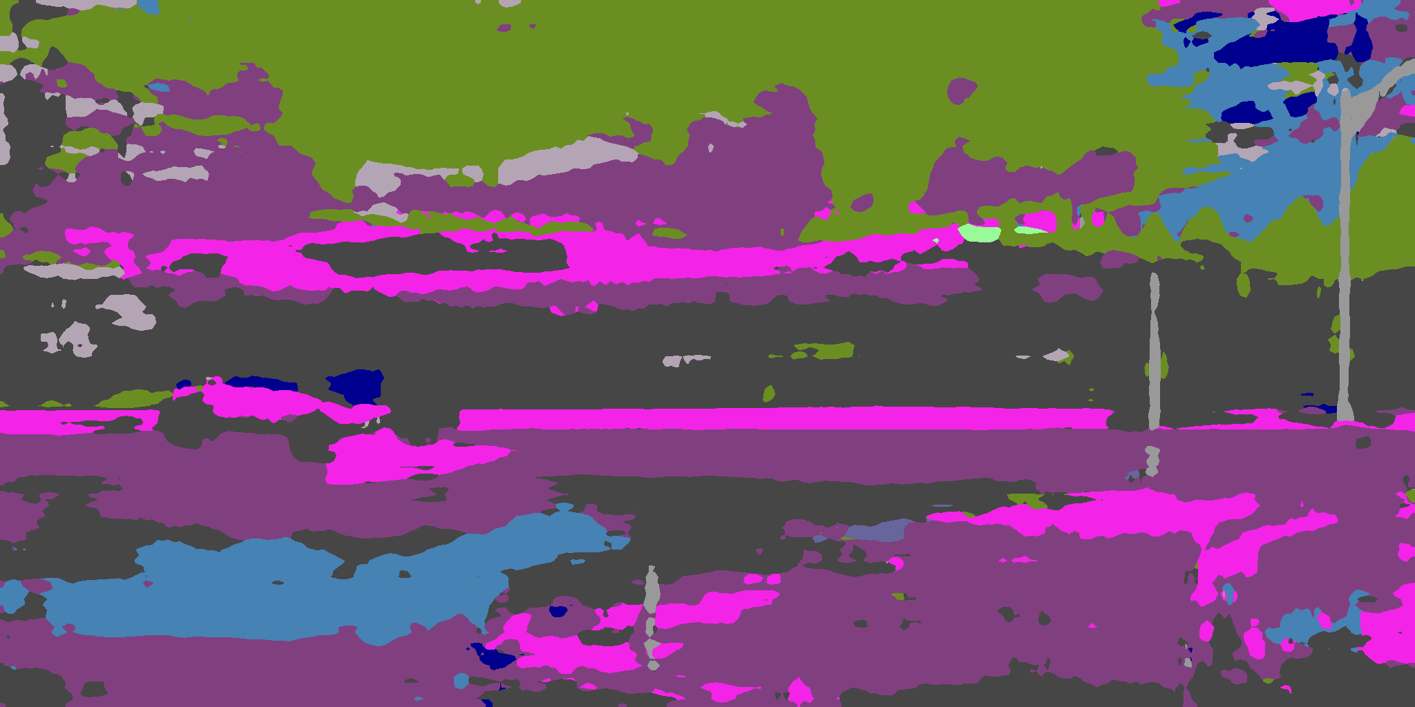
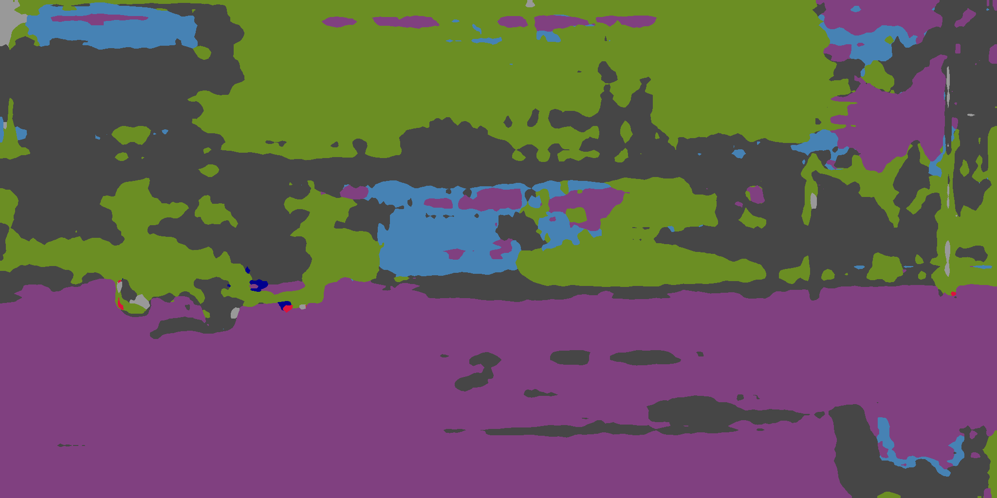
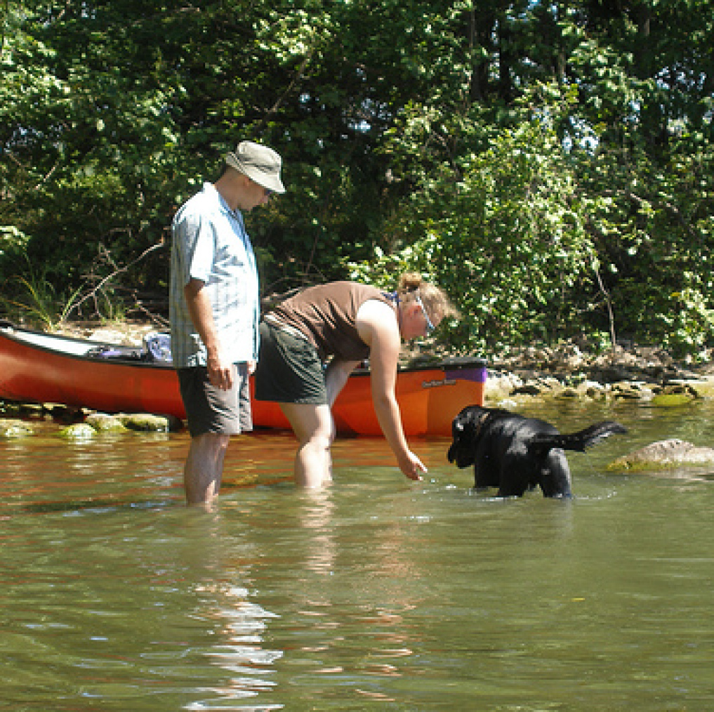
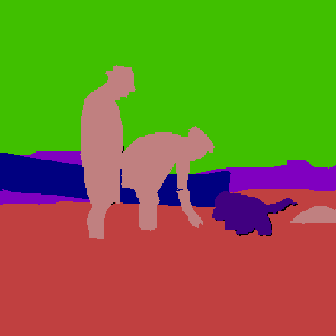
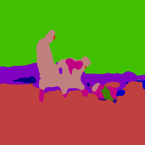
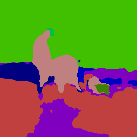
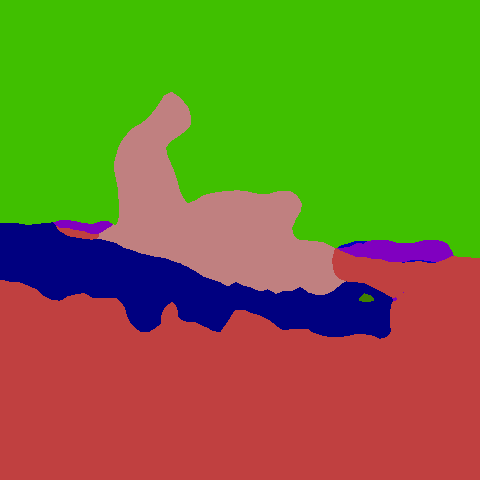
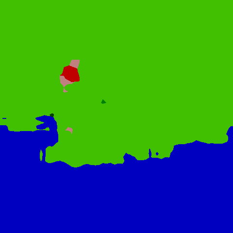
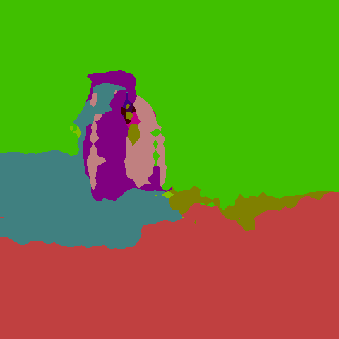
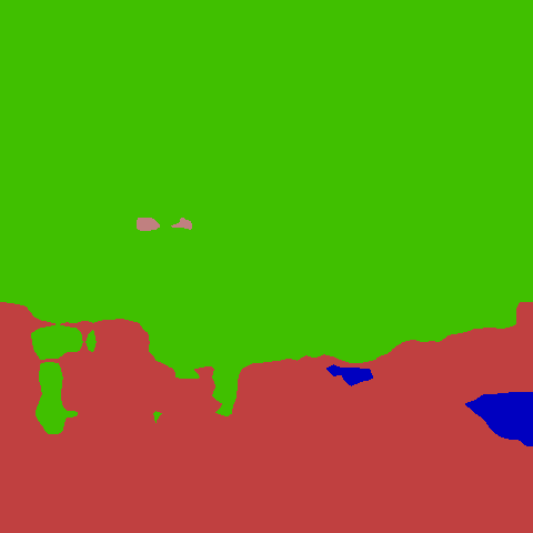
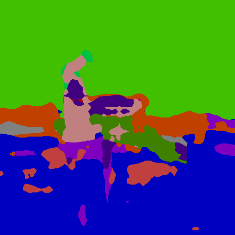
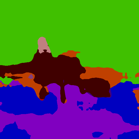
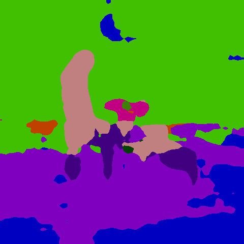
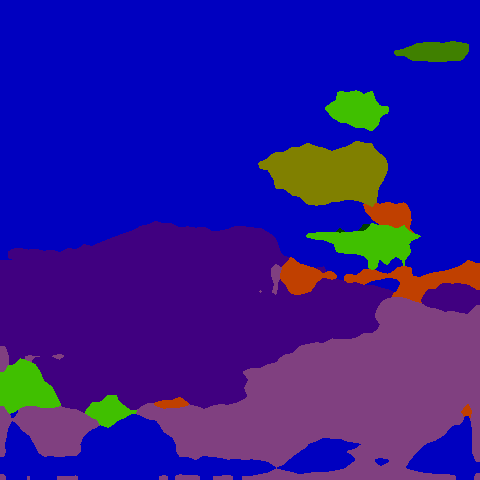
A qualitative overview of the predictions of all cue experts is shown in figs. 16, 17 and 18 for Cityscapes, CARLA and PASCAL Context, respectively. We observed for the street scene base datasets that already a non-negligible amount of information, like the position of a car, can be learned solely based on the color value of a pixel (cf. figs. 16 and 17 last row).
 |
 |
 |
|
 |
 |
 |
Cityscapes |
 |
 |
 |
|
 |
 |
 |
CARLA |
 |
 |
 |
|
 |
 |
 |
Context PASCAL |
| expert | expert | ground truth |





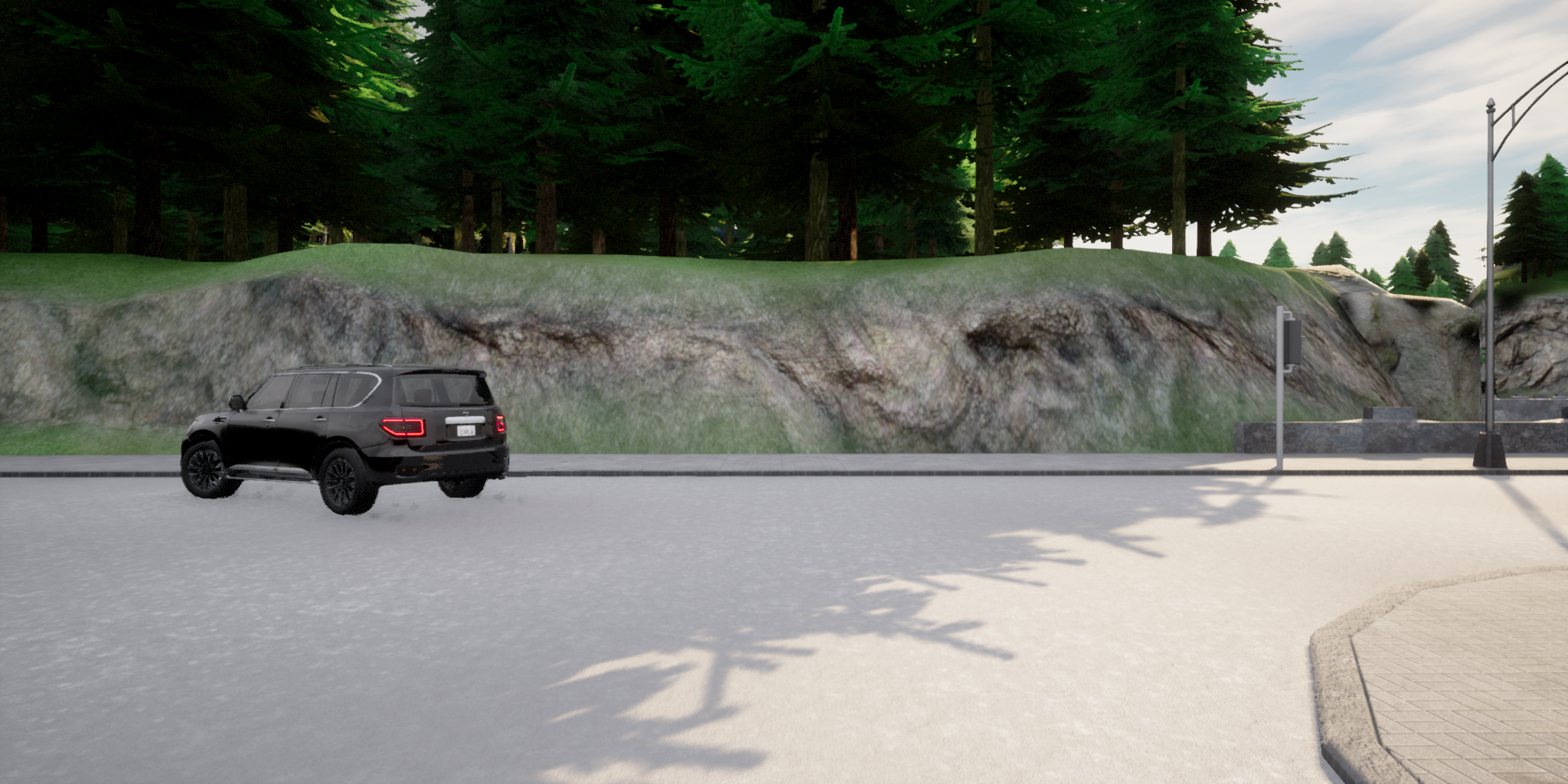
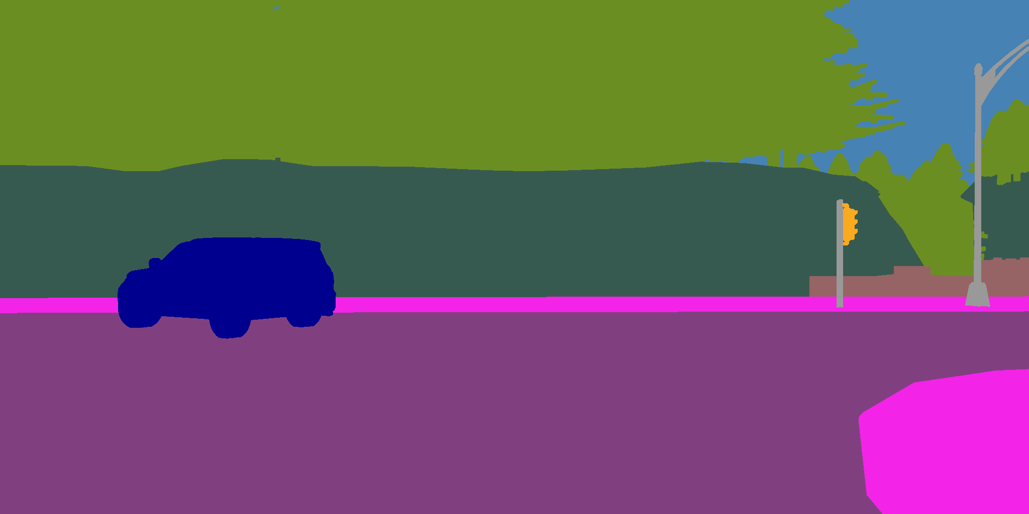
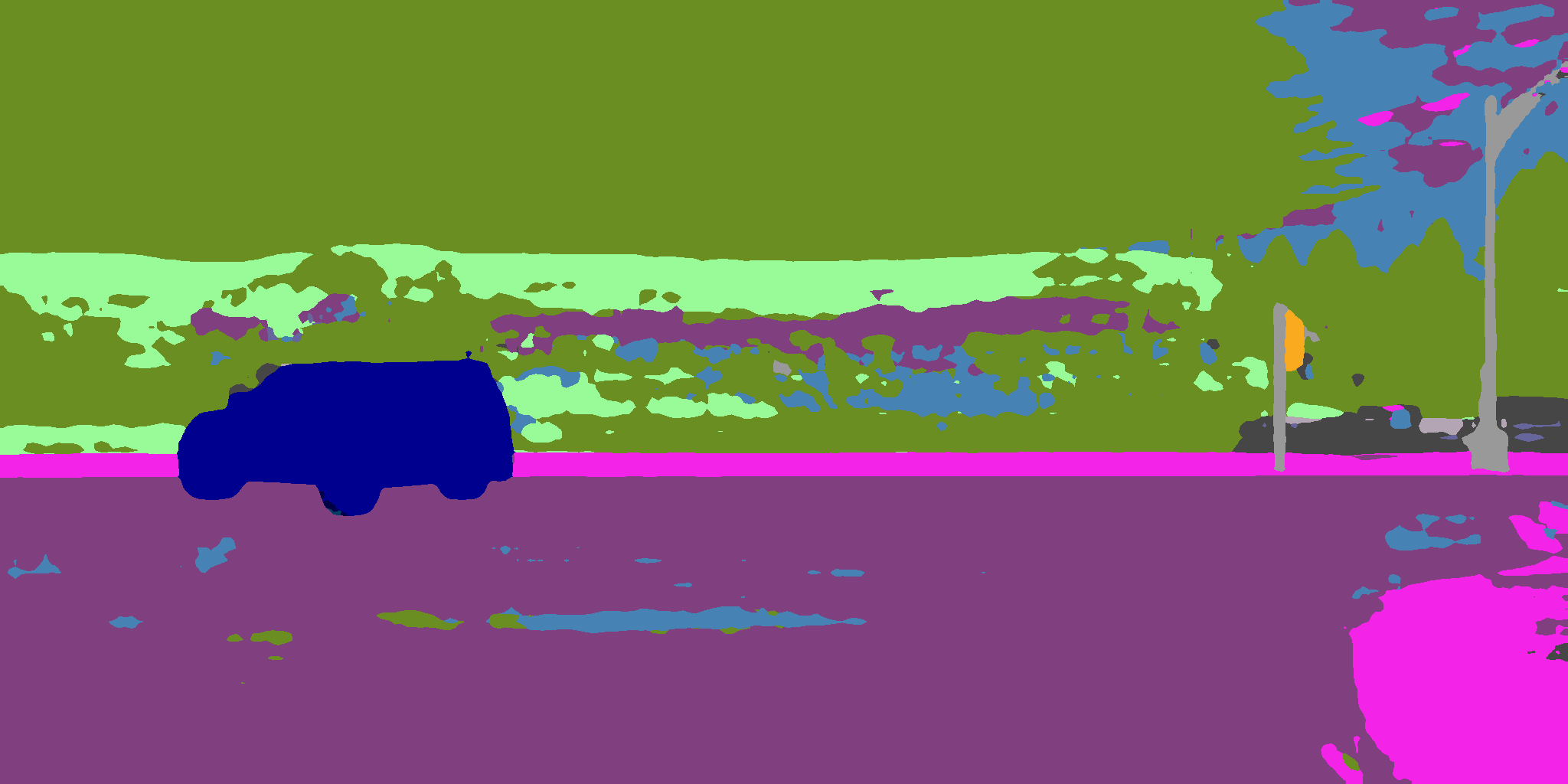
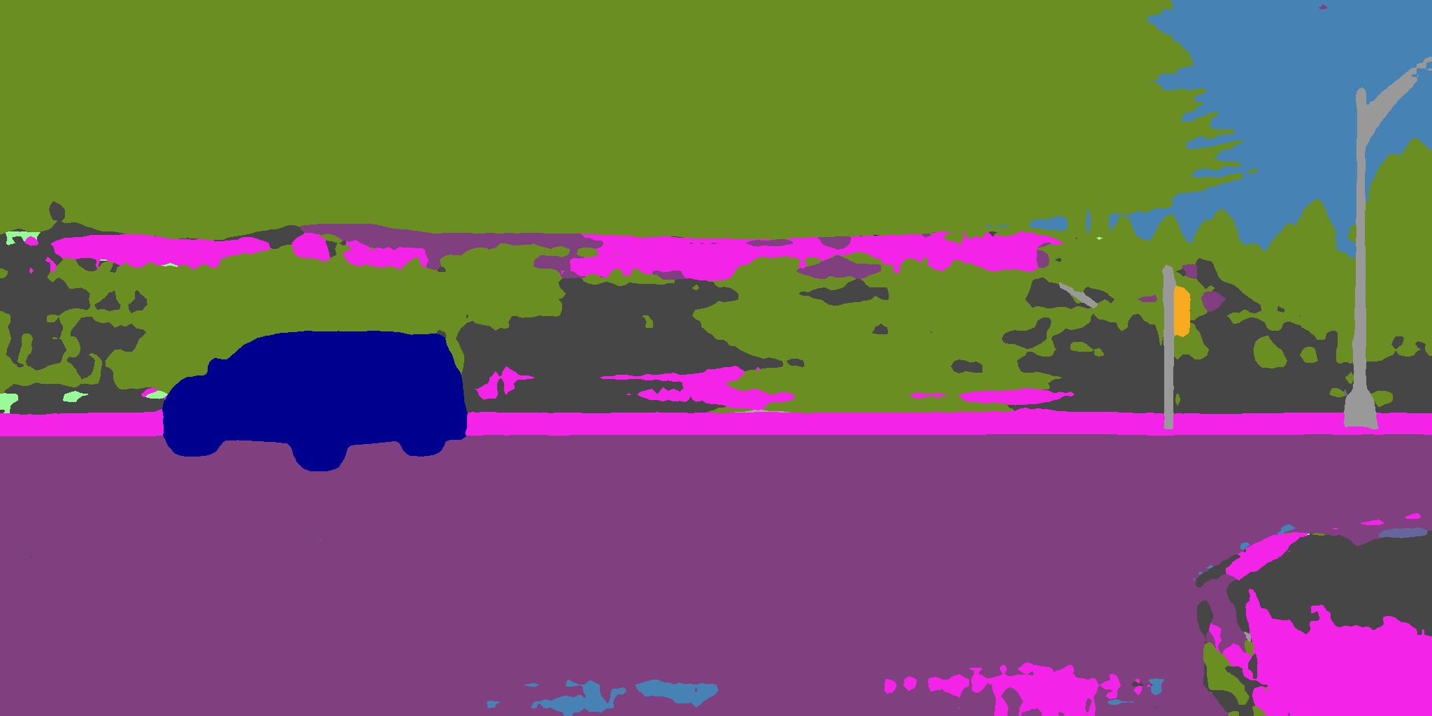


 (a) image
 (b) ground truth
 (c) all cues
 (d)
(d)
 (e)
(e)
 (f)
(f)
 (g)
(g)
 (h)
(h)
 (i)
(i)
 (j)
(j)
 (k)
(k)
 (l)
(l)
 (m) gray
 (n) HS
 (o) RGB
Cue Influence in Different Architectures.
The transformer experiments conducted on the PASCAL Context dataset demonstrate results comparable to those obtained on the Cityscapes dataset (cf. table II). These findings suggest that the influence of cues remains largely consistent between CNN and transformer architectures, as the order of cues has not experienced significant changes (see last column of table VI for reference).
| Color | CNN mIoU | CNN gap | transformer mIoU | transformer gap | change in rank | ||||
| S | T | V | HS | (%, ) | (pp., ) | (%, ) | (pp., ) | w.r.t. CNN | |
| no info | |||||||||
| V | ✓ | ||||||||
| HS | ✓ | ||||||||
| ✓ | |||||||||
| RGB | ✓ | ✓ | |||||||
| ✓ | ✓ | ||||||||
| ✓ | ✓ | ✓ | |||||||
| ✓ | ✓ | ||||||||
| ✓ | ✓ | ||||||||
| ✓ | ✓ | ||||||||
| ✓ | ✓ | ✓ | |||||||
| ✓ | ✓ | ✓ | |||||||
| ✓ | ✓ | ✓ | |||||||
| all cues | ✓ | ✓ | ✓ | ✓ | |||||