Phoebus: Performance Portable GRRMHD for Relativistic Astrophysics

Abstract

We introduce the open source code Phoebus (phifty one ergs blows up a star) for astrophysical general-relativistic radiation magnetohydrodynamic simulations. Phoebus is designed for, but not limited to, high-energy astrophysical environments such as core-collapse supernovae, neutron star mergers, black-hole accretion disks, and similar phenomena. General relativistic magnetohydrodynamics are modeled in the Valencia formulation with conservative finite volume methods. Neutrino radiation transport is included with Monte Carlo and moment methods. Phoebus is built on the parthenon (Grete et al., 2022) performance portable adaptive mesh refinement framework, uses a GPU first development strategy, and is capable of modeling a large dynamic range in space and time. Phoebus utilizes kokkos  for on-node parallelism and supports both CPU and GPU architectures. We describe the physical model employed in Phoebus, the numerical methods used, and demonstrate a suite of test problems to demonstrate its abilities. We demonstrate weak scaling to over 500 H100 GPUs.

1 Introduction

Compact objects such as neutron stars and black holes, through their formation channels or interactions with their environments, power some of the most energetic phenomena in the universe. Core-collapse supernovae (CCSNe), gamma-ray bursts, neutron star (NS) mergers, X-ray binaries, and quasars, to name a few, compose some of the most energetic phenomena observed. These events are linked to nearly all of the post-Big Bang nucleosynthesis, the chemical and dynamical evolution of galaxies, and comprise many of the compact object formation channels. Furthermore, these phenomena probe matter at its most extreme, acting as grand laboratories for fundamental physics.

Our understanding of these phenomena relies on the union of theory and observation. For the former, computational methods are an essential tool necessary for modeling the underlying physics. However, these environments each have spatial and temporal scales that span many orders of magnitude on their own. Typically, each of these domains is attacked with a specialized code, tuned for a specific problem of interest.

We present Phoebus (phifty one ergs blows up a star) , a new general-relativistic radiation magnetohydrodynamics (GRRMHD) code developed for modeling systems in relativistic astrophysics. Phoebus includes all of the physics necessary to model these systems, including accurate radiation transport for neutrino fields, constrained-transport GRMHD, a wide variety of equations of state including those of dense nuclear matter, and the ability to model a wide dynamic range in space and time through adaptive mesh refinement and a GPU-resident development strategy.

An additional challenge, separate from numerically modeling the rich physics necessary, is the need to do so efficiently, across a diverse range of computing architectures – so called performance portability. Computing resources are becoming increasingly hetereogeneous with compute nodes being comprised of both CPUs and GPUs and each GPU vendor supporting their own programming model and software stack. Hence, modern high performance simulation software must not only be able to leverage these architectures, but do so efficiently. To enable this, Phoebus is built upon parthenon , a performance portable, block-structured adaptive mesh refinement (AMR) library (Grete et al., 2022). parthenon , in turn, uses kokkos (Edwards et al., 2014; Trott et al., 2021, 2022), a hardware agnostic performance portability abstraction library, for on-node parallelism. This enables the user to, at compile time, select the target hardware, and kokkos specializes the relevant code to the hardware. kokkos also exposes fine grained tuning of loop patterns to enable platform specific optimizations.

The development of Phoebus also benefited from loose collaboration with the AthenaK (Stone et al., 2024; Zhu et al., 2024; Fields et al., 2024) team. Both projects are outgrowths of the parthenon  project and several ideas and optimizations in Phoebus were born from inter-team conversations. Phoebus and parthenon  as a whole also owe a great debt to the Athena++ code (Stone et al., 2020), from which the entire constellation of projects was born.

Phoebus adopts a fully free-and-open-source development model. Making scientific software open source constitutes good scientific practice as it enables transparency, full reproducability, and ultimately enables more science through serving the community. The code is publicly available and developed on GitHub. We welcome, and hope for, bug reporting, issue tracking, feature or pull requests, and general feedback from the community. Continuous integration and unit testing are enabled with the Catch2 unit testing framework and all pull requests are reviewed before merging into the main codebase. Phoebus includes an expansive, and growing, suite of unit and regression tests that stress simple compilations and functionalities to large multiphysics problems. The software is licensed under the 3-clause Berkeley Software Distribution (BSD-3) clause which has relaxed rules for distribution.

In Section 2 we lay out the full system of equations that Phoebus is currently designed to solve. In Section 3 we describe the numerical methods used for each physics sector. In Section 4 we present a suite of tests designed to stress and verify the fidelity of Phoebus. We briefly discuss the parallel performance of Phoebus in Section 5. Finally we offer concluding thoughts in Section 6 and discuss the future direction of Phoebus as well as its position as an open-source software.

2 Physical Model

In Phoebus we adopt the general relativistic Euler equations of magnetohydrodynamics, supplemented by an appropriate, but flexible, equation of state. We include neutrino transport with moment and Monte Carlo methods. The relevant systems of equations and physical assumptions are given below. In all of the following, Greek indices run from 0 to 3 and Latin indices run from 1 to 3. We adopt the Einstein summation convention for repeated indices.

2.1 GRRMHD

For the fluid equations, we adopt the Valencia Formulation (Banyuls et al., 1997; Font et al., 2000) as summarized in Giacomazzo & Rezzolla (2007). We solve the conservation law

$$(\sqrt{\gamma}\mathbf{U})_{,t}+(\sqrt{-g}\mathbf{F}^{i})_{,i}=\sqrt{-g}\mathbf{S}$$ (1)

for conserved vector

$$\mathbf{U}=\begin{pmatrix}D\\ S_{j}\\ \tau\\ B^{k}\end{pmatrix}=\begin{pmatrix}\rho W\\ (\rho h+b^{2})W^{2}v_{j}-\alpha b^{0}b_{j}\\ (\rho h+b^{2})W^{2}-(p+b^{2}/2)-\alpha^{2}(b^{0})^{2}-D\\ B^{k}\end{pmatrix},$$ (2)

flux vector

$$\mathbf{F}^{i}=\begin{pmatrix}D\tilde{v}^{i}/\alpha\\ S_{j}\tilde{v}^{i}/\alpha+(p+b^{2}/2)\delta^{i}_{j}-b_{j}B^{i}/W\\ \tau\tilde{v}^{i}/\alpha+(p+b^{2}/2)v^{i}-\alpha b^{0}B^{i}/W\\ B^{k}\tilde{v}^{i}/\alpha-B^{i}\tilde{v}^{k}/\alpha\end{pmatrix},$$ (3)

and source vector

$$\mathbf{S}=\begin{pmatrix}0\\ T^{\mu\nu}(g_{\nu j,\mu}-\Gamma^{\delta}_{\nu\mu}g_{\delta j})+G_{\nu}\\ \alpha(T^{\mu 0}(\ln\alpha)_{,\mu}-T^{\mu\nu}\Gamma^{0}_{\nu\mu})+G_{\nu}\\ 0^{k}\end{pmatrix},$$ (4)

where $u^{\mu}$ is the four-velocity of the fluid,

$$v^{i}=\frac{u^{i}}{W}+\frac{\beta^{i}}{\alpha}$$ (5)

is the 3-velocity, with densitized 3-velocity

$$\tilde{v}^{i}=\alpha v^{i}-\beta^{i},$$ (6)

for Lorentz factor

$$W=\alpha u^{0},$$ (7)

lapse $\alpha$, shift $\beta^{i}$, magnetic field four-vector $b^{\mu}$ defined by

$$b^{\mu}u^{n}u-b^{\nu}u^{m}u=*F^{\mu\nu}$$ (8)

for the Hodge star of the Maxwell stress tensor $*F^{\mu\nu}$, baryon number density $\rho$, specific enthalpy $h$, Christoffel symbols $\Gamma^{\mu}_{\nu\sigma}$, four-metric $g_{\mu\nu}$, three-metric $\gamma_{\mu\nu}$, and stress-energy tensor

$$T^{\mu\nu}=(\rho+u+P+b^{2})u^{\mu}u^{\nu}+\left(P+\frac{1}{2}b^{2}\right)g^{\mu\nu}-b^{\mu}b^{\nu},$$ (9)

for pressure $P$. $G_{\nu}$ is the radiation 4-force including radiation-matter interactions. The magnetic field four-vector $b^{\mu}$ is related to the Eulerian observer magnetic field 3-vector $B^{i}$ by

$$b^{0} = \frac{W}{\alpha}B^{i}v_{i}$$ (10)

$$b^{i} = \frac{B^{i}+\alpha b^{0}u^{i}}{W}$$ (11)

$$b^{2} = b^{\mu}b_{\mu}=\frac{B^{2}+\alpha^{2}(b^{0})^{2}}{W^{2}}.$$ (12)

We also track a primitive vector

$$\mathbf{P}=\begin{pmatrix}\rho\\ Wv^{i}\\ \rho\epsilon\\ B^{k}\end{pmatrix},$$ (13)

which is used for reconstructions and to compute fluxes.

In addition to the above equations, Phoebus supports the evolution of arbitrary passive scalars

$$\left(X\rho u^{\mu}\right)_{;\mu}=S$$ (14)

where $X$ is some advected quantity that is neither intrinsic nor extrinsic, $S$, is some potentially non-zero source term, and the notation $\phi^{\mu}_{;\mu}$ denotes the covariant derivative. In Phoebus, we use this framework to model the lepton exchange between the matter and neutrino radiation fields, taking $X$ to be the electron fraction $Y_{e}$ and $S$ to be $\sqrt{-g}G_{ye}$, with $G_{ye}$ capturing the rate of transfer.

2.2 Equation of State

The equation of state (EOS) provides the relationship between the independent and thermodynamic variables and, in general, encapsulates much of the required microphysics. These dependent variables, and on occasion their derivatives, are crucial for modeling astrophysical environments. Phoebus supports a wide range of equations of state of astrophysical interest, including tabulated dense matter and stellar equations of state.

Software capable of modeling a range of astrophysical environments requires flexibility in its EOS. To this end, the EOS functionality of Phoebus is provided by an external library, singularity-eos  (Miller et al., submitted to JOSS). singularity-eos provides downstream fluid codes with performance portable EOS access with a unified API across all EOS’s. At present, singularity-eos implements more than ten EOS’s including, of note, ideal gas, Helmholtz (Timmes & Swesty, 2000), and tabulated dense matter. Implementing the EOS microphysics with this framework allows us to switch, or add, EOS’s without modifying Phoebus. singularity-eos provides one-to-one Python bindings for testing and analysis. We support the ability to solve for adiabats of an arbitrary EOS – a crucial capability as many initial condition setups require constant entropy.

In this work we use either an ideal equation of state or a tabulated nuclear matter EOS. For the latter we use the “SFHo” EOS (Steiner et al., 2013a). SFHo is a relativistic mean field model built upon Hempel et al. (2012) that, importantly, was constructed to reproduce observed neutron star mass-radius relationships.

2.3 Gravity

Phoebus is a fully general relativistic code, and gravity is implemented via the curvature of a metric tensor. We implement a generic metric infrastructure that supports a selection of tabulated, analytically prescribed, and numerically computed metrics at compile time. The machinery is highly flexible, allowing for simple compile-time switching of metric implementations. We provide a method GetCoordinateSystem, which returns a CoordinateSystem object. This object has reference semantics, but can be copied safely to device, similar to Kokkos::Views. Depending on user selection at compile time, requesting, e.g., the spatial metric $\gamma_{ij}$ from the CoordinateSystem object may reference an evolved grid variable, an analytic formula, or tabulated data. Derivatives, such as those needed for Christoffel symbols may be computed either analytically or numerically via finite differences.

2.3.1 Monopole GR

For problems where gravitational waves aren’t dynamically important and where the gravitational potential is approximately spherically symmetric, Phoebus provides a monopole solver, which assumes a spherically symmetric 3-metric with maximal slicing and areal shift

$$ds^{2}=(-\alpha^{2}+a^{2}(\beta^{r})^{2})dt^{2}+2a^{2}\beta^{r}dtdr+a^{2}dr^{2}+r^{2}d\Omega^{2}.$$ (15)

with unknown metric function $a$, lapse $\alpha$, and radial shift $\beta^{r}$.

It turns out that in spherical symmetry, under these gauge conditions, the Einstein constraint equations are sufficient to specify the metric and extrinsic curvature components $a$ and $K^{r}_{r}$. The Hamiltonian constraint provides an equation for $a$ and the momentum constraint for $K^{r}_{r}$:

$$\partial_{r}a = \frac{a}{8r}\left\{4+a^{2}\left[-4+r^{2}\left(3(K^{r}_{r})^{2}+32\pi\rho_{\rm ADM}\right)\right]\right\}$$ (16)

$$\partial_{r}K^{r}_{r} = 8\pi a^{2}j^{r}-\frac{3}{r}K^{r}_{r}.$$ (17)

Here

$$\rho=\tau+D$$ (18)

is the ADM mass and

$$j^{i}=S^{i}$$ (19)

is the ADM momentum. The ADM evolution equations can then be used to solve for the gauge variables, $\alpha$ and $\beta^{r}$:

$$\frac{1}{a^{2}}\partial^{2}_{r}\alpha = \alpha\left[\frac{3}{2}(K^{r}_{r})^{2}+4\pi(\rho+S)\right]+\frac{a^{\prime}}{a^{3}}\partial_{r}\alpha-\frac{2}{a^{2}r}\partial_{r}\alpha$$ (20)

$$\beta^{r} = -\frac{1}{2}\alpha rK^{r}_{r},$$ (21)

where the lapse $\alpha$ satisfies a second-order boundary-value problem, and the shift $\beta$ is given algebraically. Here

$$S^{i}_{j}=(\rho_{0}h+b^{2})W^{2}+3(P+b^{2}/2)-P^{i}_{\mu}P_{j}^{\nu}b^{\mu}b_{\nu}$$ (22)

is the ADM stress tensor and $P$ is the projection operator onto the hypersurface of constant coordinate time.

The boundary conditions are given by symmetry at the origin,

$$a(r=0) = 1$$ (23)

$$K^{r}_{r}(r=0) = 0$$ (24)

$$\partial_{r}\alpha(r=0) = 0,$$ (25)

and the weak field limit at large radii:

$$\lim_{r\to\infty}\alpha = 1-\frac{c}{r}$$ (26)

$$\Rightarrow\lim_{r\to\infty}\partial_{r}\alpha = \frac{c}{r^{2}}$$ (27)

$$\Rightarrow\lim_{r\to\infty}\alpha = 1-r\partial_{r}\alpha.$$ (28)

We solve equations (16) and (17) by integration outward from the origin using a second-order Runge-Kutta method. If Equation (20) is discretized by second-order centered finite differences, it forms a matrix equation, where the matrix operator is tridiagonal. This operator may then be inverted via standard diagonal matrix inversion techniques.

To complete the monopole solver, time derivatives of the metric must be provided so that the time-components of the Christoffel symbols may be provided by the infrastructure. These equations are algebraically complex, and so are not included here. They are summarized in Appendix A.

2.4 Radiation

In many problems of interest in relativistic astrophysics it is necessary to consider radiation fields and their impact on the matter field. These radiation fields may exchange four-momentum and, in the case of neutrino radiation, lepton number with the matter field. Here, we focus primarily on neutrino radiation.

The species-dependent neutrino distribution function $f_{\nu}(x^{\alpha},p^{\alpha})$, for 4-position and 4-momentum $x^{\alpha}$ and $p^{\alpha}$, evolves according to the 6+1 Boltzmann equation

$$p^{\alpha}\left[\frac{\partial f_{\nu}}{\partial x^{\alpha}}-\Gamma^{\beta}_{\alpha\gamma}p^{\gamma}\frac{\partial f_{\nu}}{\partial p^{\beta}}\right]=\left[\frac{df_{\nu}}{d\tau}\right]_{\rm{coll}}$$ (29)

where $\Gamma^{\beta}_{\alpha\gamma}p^{\gamma}$ are the Christoffel symbols and the right hand side is the collision term including neutrino-matter interactions. Full solution of the 6+1 Boltzmann equation in dynamical environments remains computationally intractable for mesh-bashed methods and simplifications must be made, as we discuss in detail in Section 3.3.

Type	Processes	Current	Corrections/Approximations
Abs./Emis. on neutrons	$\nu_{e}+n\leftrightarrow e^{-}+p$ $\nu_{\mu}+n\leftrightarrow\mu^{-}+p$	Charged	Blocking/Stimulated Abs. Weak Magnetism Kinematic recoil
Abs./Emis. on protons	$\bar{\nu}_{e}+p\leftrightarrow e^{+}+n$ $\bar{\nu}_{\mu}+p\leftrightarrow\mu^{+}+n$	Charged	Blocking/Stimulated Abs. Weak Magnetism Kinematic recoil
Abs./Emis. on ions	$\nu_{e}A\leftrightarrow A^{\prime}e^{-}$	Charged	Blocking/Stimulated Abs. Kinematic recoil
Electron capture on ions	$e^{-}+A\leftrightarrow A^{\prime}+\nu_{e}$	Charged	Blocking/Stimulated Abs. Kinematic recoil
$e^{+}-e^{-}$ Annihilation	$e^{+}e^{-}\leftrightarrow\nu_{i}\bar{\nu}_{i}$	Charged + Neutral	single-$\nu$ Blocking Kinematic recoil
$n_{i}$-$n_{i}$ Brehmsstrahlung	$n_{i}^{1}+n_{i}^{2}\to n_{i}^{3}+n_{i}^{4}+\nu_{i}\bar{\nu}_{i}$	Neutral	single-$\nu$ Blocking Kinematic recoil

Table 1: Emission and absorption processes used in Phoebus. Reproduced from (Miller et al., 2019).

We include a suite of relevant neutrino-matter interactions. We list the absorption and emission processes in Table 1. Those absorption and emission interactions involving electron type neutrinos and antineutrinos will exchange lepton number with the fluid, modifying the composition. We include the elastic scattering processes listed below,

$$\nu_{i}+p \leftrightarrow \nu_{i}+p$$ (30)

$$\nu_{i}+n \leftrightarrow \nu_{i}+n$$ (31)

$$\nu_{i}+A \leftrightarrow \nu_{i}+A$$ (32)

$$\nu_{i}+\alpha \leftrightarrow \nu_{i}+\alpha$$ (33)

where $n$ represent neutrons, $p$ protons, $\nu_{i}$ neutrinos, $A$ heavy ions, and $\alpha$ alpha particles. Emissivities and opacities are tabulated as presented in Burrows et al. (2006).

The above set of interactions, while sufficient for many applications, is not exhaustive. In particular, we neglect neutrino-electron inelastic scattering (Bruenn, 1985). Experience has repeatedly demonstrated that even small corrections can have a large impact on neutrino-matter interactions and the subsequent dynamics (e.g., Freedman, 1974; Arnett, 1977; Bethe & Wilson, 1985; Bruenn, 1985; Horowitz, 1997; Burrows & Sawyer, 1998; Reddy et al., 1998; Müller et al., 2012; Buras et al., 2003; Hix et al., 2003; Kotake et al., 2018; Bollig et al., 2017; Fischer et al., 2020; Betranhandy & O’Connor, 2020; Miller et al., 2020; Kuroda, 2021). Future work for production simulations will include more complete sets of neutrino-matter interactions.

Neutrinos exchange four-momentum and lepton number with the fluid. In a frame co-moving with the fluid, the four-momentum source term is given as

$$G_{(a)}=\frac{1}{h}\int(\chi_{\epsilon,f}I_{\epsilon,f}-\eta_{\epsilon,f})n_{(a)}d\epsilon d\Omega,$$ (34)

where $\chi_{\epsilon,f}=\alpha_{\epsilon,f}+\sigma_{\epsilon,f}^{a}$ is the flavor dependent extinction coefficient combining absorption $\alpha_{\epsilon,f}$ and scattering $\sigma_{\epsilon,f}^{a}$, $I_{\epsilon,f}$ is the radiation intensity, $\eta_{\epsilon,f}=j_{\epsilon,f}+\eta_{\epsilon,f}^{s}(I_{\epsilon,f})$ is the total emissivity combining fluid $j_{\epsilon,f}$ and scattering $\eta_{\epsilon,f}^{s}$ emission, and $n_{(a)}=p_{(a)}/\epsilon$. This is then mapped into the lab frame by a coordinate transformation

$$G^{\mu}=e^{\mu}_{(a)}G^{(a)}$$ (35)

where $e^{\mu}_{(a)}$ defines an orthonormal tetrad.

The lepton number exchange source term $G_{ye}$ is given by

$$G_{ye}=\frac{m_{p}}{h}\textrm{sign}(f)\int\frac{\chi_{\epsilon,f}I_{\epsilon,f}-\eta_{\epsilon,f}}{\epsilon}d\epsilon d\Omega$$ (36)

where $m_{p}$ is the proton mass and

$$\textrm{sign}(f)=\begin{cases}1&\text{for}\ f=\nu_{e}\\ -1&\text{for}\ f=\bar{\nu}_{e}\\ 0&\text{for}\ f=\nu_{x}\end{cases}$$ (37)

determines the sign of the lepton exchange.

3 Numerical Methods

Here we lay out the numerical methods used to solve the equations introduced above.

3.1 MHD

Evolution of conserved fluid quantities is done with a standard second order finite volumes scheme. Magnetic field evolution is included in Phoebus using a constrained transport scheme described in Tóth (2000). This formulation of constrained transport uses cell centered magnetic fields. For further details on the formulations used in Phoebus, see Miller et al. (2019); Gammie et al. (2003). The details of magnetic field treatment will be the subject of future updates to Phoebus.

Phoebus currently supports the local Lax-Friedrichs (LLF) and Harten-Lax-van Leer (HLL) Riemann solvers (Harten et al., 1983; Toro, 2009). Additional Riemann solvers are planned to be supported in the future. Reconstruction methods currently supported in Phoebus include piecewise constant (denoted constant); piecewise linear (denoted linear) with a variety of limiter options, though the default is minmod (Van Leer, 1977; Roe, 1986; Kuzmin, 2006); the fifth-order monotonicity preserving scheme of Suresh & Huynh (1997) (denoted mp5); and a novel fifth-order weighted essentially non-oscillatory (Shu, 2009, WENO) implementation using the Z-type smoothness indicators from Borges et al. (2008) (denoted WENO5-Z-AOAH) that mixes a high-order WENO5-Z reconstruction with a low order piecewise linear reconstruction. We call this WENO scheme WENO5-Z-AOAH, and describe it in detail in Appendix B.

The recovery of the primitive variables from the conserved state vector is non-trivial, and must be computed numerically, as no analytic solution is available. We use the procedure described in Kastaun et al. (2021), which is guaranteed to always converge.

3.2 Atmosphere Treatment

Numerical modeling of accretion disk systems requires including vacuum originally outside of the disk – a feat infeasible for Eulerian hydrodynamics. Instead, artificial atmospheres must be imposed to ensure both physical validity and stability of the numerical scheme. The problem is further complicated by the use of a tabulated equation of state which has strict bounds on the range of grid variables. In general, an EOS with a set of $n$ state variables $\mathcal{Q}$ has bounds

$$\mathcal{Q}_{i}\in\{q_{\rm min},q_{\rm max}\}\,\,\text{for}\,i=1,\dots,n$$ (38)

For the Helmholtz EOS, take $\mathcal{Q}=\{\rho,T\}$. Including electron fraction $Y_{e}$ allows for tabulated nuclear matter EOS’s commonly used for CCSN and merger simulations such as SFHo. These bounds must be accounted for. We demand that density remain above some floor value, i.e., $\rho>\rho_{\rm flr}$. There are several implemented forms for the floor density, including

$\centering\rho_{\rm flr}=\left\{\begin{array}[]{c}\rho_{0}\\ \rho_{0}e^{-\alpha x^{1}}\\ \rho_{0}(x^{1})^{-\alpha}\\ \rho_{0}r^{-\alpha}\end{array}\right.\@add@centering$

where $\rho_{0}$ is some small, problem dependent constant and $\alpha$ is a positive exponent. $x^{1}$ is the radial coordinate which, depending on the coordinate system, may be transformed (e.g., $x^{1}=$ ln$(r)$). We generally take $\alpha=2.0$, but that is not required. For black hole accretion problems, the density floor near a black hole is approximately $\rho_{0}$ and, besides the first constant case, decays with radius. This radial decay ensures that the floors do not interfere with winds from the disk. To ensure consistency with the tabulated EOS, we require that the floor does not extend below the minimum density in the table. The specific internal energy is set similarly to the above. For electron fraction we simply require that it stay within the bounds of the table. In general in Phoebus we use the second case, where relevant, unless otherwise noted.

3.3 Radiation

In contexts such as BNS mergers and CCSNe, neutrinos are responsible for exchanging four-momentum and lepton number with the fluid. Neutrino-matter interactions drive the chemical and dynamical evolution of these systems, with electron neutrino absorption (emission) driving the matter to be more proton (neutron) rich, and inversely for electron anti-neutrinos. An accurate treatment of the neutrino radiation field is necessary for following nucleosynthesis in problems of interest.

We implement in Phoebus several methods for evolving the radiation fields. First, we include a gray, two moment approach. Additionally, following closely to the methods outlined in bhlight and nubhlight (Dolence et al., 2009; Ryan et al., 2015; Miller et al., 2019), we implement neutrino transport through Monte Carlo methods. There is also, for testing purposes, a simple “lightbulb” approach where the neutrino luminosity is fixed at a constant value and a analytic form for the source terms is taken (similar to, e.g., Janka, 2001). We do not discuss that approach here. Implementation of the method of characteristics moment closure approach of Ryan & Dolence (2020) for neutrino transport is in progress, but discussion delayed for the moment.

For all of the above we consider three neutrino flavors: electron neutrinos, electron antineutrinos, and a characteristic heavy neutrino. With appropriate microphysics, the methods may be trivially extended to include, for example, muon neutrino evolution. Below we summarize the methods included in Phoebus and refer the reader to the aforementioned works for further details.

3.3.1 Monte Carlo

The probability distribution of emitted Monte Carlo packets is

$$\frac{1}{\sqrt{-g}}\frac{dN_{p}}{d^{3}xdtd\nu d\Omega}=\frac{1}{\omega\sqrt{-g}}\frac{dN}{d^{3}xdtd\nu d\Omega}=\frac{1}{w}\frac{j_{\nu,f}}{h\nu}$$ (39)

where $N_{p}$ is the number of Monte Carlo packets with $\omega$ physical neutrinos per packet, $N$ is the number of physical particles, $j_{\nu,f}$ is the fluid frame emissivity of neutrinos with frequency $\nu$, and flavor $f\in\{\nu_{e},\bar{\nu}_{e},\nu_{x}\}$, and $h$ is Planck’s constant. The number of emitted packets in timestep $\Delta t$ is

$$N_{p,tot}=\Delta t\sum_{f}\int\sqrt{-g}d^{3}xd\nu d\Omega\frac{1}{w}\frac{j_{\nu,f}}{h\nu}$$ (40)

and the number of packets of flavor $f$ created in a computational cell $i$ of volume $\Delta^{3}x$ is

$$N_{p,f,i}=\Delta t\Delta^{3}x\int\sqrt{-g}d\nu d\Omega\frac{1}{w}\frac{j_{\nu,f}}{h\nu}.$$ (41)

We control the total number of Monte Carlo packets created per timestep by setting the weights $w$ as

$$w=\frac{C}{\nu}$$ (42)

where C is a constant. This ensures that packets of frequency $\nu$ and weight $w(\nu)$ have energy

$$E_{p}=wh\nu=hC,$$ (43)

such that packet energy is independent of frequency. The constant $C$ is set by fixing the total number of Monte Carlo packets created to be $N_{target}$ and setting $C$ such that equation 40 is satisfied. $N_{target}$ is set such that the total number of Monte Carlo packets is roughly constant in time. Thus, we have

$$C=\frac{\Delta t}{hN_{target}}\sum_{f}\int\sqrt{-g}d^{3}xd\nu d\Omega j_{\nu,f}.$$ (44)

Absorption of radiation is treated probabilistically in Monte Carlo fashion. A neutrino of flavor $f$ that travels a distance $\Delta\lambda$ traverses an optical depth

$$\Delta\tau_{a,f}(\nu)=\nu\alpha_{\nu,f}\Delta\lambda$$ (45)

where $\alpha_{\nu,f}$ is the absorption extinction coefficient for radiation of frequency $\nu$ and flavor $f$. Absorption occurs if

$$\Delta\tau_{a,f}(\nu)>-\rm{ln}(r_{a})$$ (46)

where $r_{a}$ is a random variable sampled uniformly from the interval [0, 1).

The implementation of Monte Carlo radiation leverages parthenon ’s swarms particle infrastructure. Monte Carlo scattering is not yet implemented in Phoebus. In the future, Monte Carlo scattering will be implemented following the methods in Miller et al. (2019).

3.3.2 Moments

We implement gray M1 moments scheme in Phoebus (Thorne, 1981; Shibata et al., 2011; Cardall et al., 2013; Foucart et al., 2015). We evolve three independent neutrino species: $\nu_{e}$, $\overline{\nu}_{e}$, and $\nu_{x}$, where the latter is the combination of ($\nu_{\mu}$, $\overline{\nu}_{\mu}$, $\nu_{\tau}$, $\overline{\nu}_{\tau}$). In gray approximation we consider energy-integrated moments and evolve first two moments. The energy density, flux, and radiation pressure in the inertial frame are defined as follows

$$E=\int\epsilon f_{\nu}(p^{\mu},x^{\mu})\delta(h\nu-\epsilon)d^{3}p\,,$$ (47)

$$F^{i}=\int p^{i}f_{\nu}(p^{\mu},x^{\mu})\delta(h\nu-\epsilon)d^{3}p\,,$$ (48)

$$P^{ij}=\int\frac{p^{i}p^{j}}{\epsilon}f_{\nu}(p^{\mu},x^{\mu})\delta(h\nu-\epsilon)d^{3}p\,,$$ (49)

where $\epsilon$ is neutrino energy in the rest frame of medium. To obtain evolution equations, we decompose the stress-energy tensor for the radiation field as follows

$$T_{\rm rad}^{\mu\nu}=n^{\mu}n^{\nu}E+n^{\mu}F^{\nu}+n^{\nu}F^{\mu}+P^{\mu\nu}\,,$$ (50)

Then the conservation equations in Valencia formalism are

$$\partial_{t} (\sqrt{\gamma}E)+\partial_{i}[\sqrt{\gamma}(\alpha F^{i}-\beta^{i}E)]=\alpha\sqrt{\gamma}(\alpha G^{0}$$

$$- F^{i}\partial_{i}\alpha+P^{ij}K_{ij})\,,$$

$$\partial_{t} (\sqrt{\gamma}F_{i})+\partial_{j}[\sqrt{\gamma}(\alpha P^{j}_{i}-\beta^{j}F_{i})]=\sqrt{\gamma}(\alpha\gamma_{i\nu}G^{\nu}$$

$$+ F^{j}\partial_{i}\beta_{j}+P^{jk}\frac{\alpha}{2}\partial_{i}\gamma_{jk}-E\partial_{i}\alpha)\,,$$

where $\alpha$ is the lapse, $\beta$ is the shift, $\gamma$ is a three-metric, and $K$ is the extrinsic curvature. The first terms on the right side of Equations (3.3.2) & (3.3.2) are the collisional source terms. We consider absorption, emission, and iso-energetic scattering from the background fluid. The source terms are very similar to those in Shibata et al. (2011) and Foucart et al. (2015):

$$G=\kappa_{J}(J^{\rm eq}-J)\,,$$ (53)

$$G_{\nu}=\kappa_{J}u_{\nu}(J^{\rm eq}-J)-\kappa_{H}H_{\nu}\,,$$ (54)

where $J$ and $H_{\nu}$ are the energy and flux in the fluid rest frame. $\kappa_{J}$ is energy-averaged absorption and $\kappa_{H}$ is the sum of energy-averaged absorption and scattering opacities. $J^{\rm eq}$ is evaluated from the equilibrium distribution function

$$J^{\rm eq}=\int_{0}^{\infty}d\nu\nu^{3}\int d\Omega\frac{1}{1+exp[(\nu-\mu_{\nu})/T_{\nu}]}\,,$$ (55)

where $\mu_{\nu}$ and $T_{\nu}$ are the chemical potential and temperature of neutrinos that are in thermal equilibrium with matter, and $\nu$ is neutrino energy in the fluid frame.

To close the system of equations, we need to specify the closure relation, $P^{ij}(E,F^{i})$. We use M1 closure which evaluates $P^{ij}$ by interpolating between optically thin and optically thick regimes (Shibata et al., 2011)

$$P^{ij}=\frac{3\chi(f)-1}{2}P^{ij}_{\rm thin}+\frac{3(1-\chi(f))}{2}P^{ij}_{\rm thick}\,,$$ (56)

where $f=\sqrt{F^{\alpha}F_{\alpha})/E}$ is the flux factor and ranges from $0$ to $1$ and $\chi$ is an interpolant. We use maximum entropy closure for fermionic radiation (MEFD) which derives the closure relation by maximizing the entropy for Fermi-Dirac distribution (Cernohorsky & Bludman, 1994). In the limit of maximum packing, the MEFD closure is (Smit et al., 2000)

$$\chi=\frac{1}{3}(1-2f+4f^{2})\,.$$ (57)

Since $P^{ij}$ is a function of $f$ and $f$ is a function of $E$ and $F^{\alpha}$, we use Newton-Raphson iteration algorithm to find the roots.

We solve Equations (3.3.2) & (3.3.2) by performing a backward Euler discretization. We fix $J_{\rm BB}$, $\kappa_{J}$, $\kappa_{H}$ and obtain a linear system of equations for ($E,F_{i}$) at time ($n+1$)

$$\sqrt{\gamma}\frac{E^{n+1}-E^{*}}{\Delta t}=-\alpha\sqrt{\gamma}n^{\nu}G_{\nu}$$ (58)

$$\sqrt{\gamma}\frac{F_{i}^{n+1}-F_{i}^{*}}{\Delta t}=-\alpha\sqrt{\gamma}\gamma_{i}^{\nu}G_{\nu}$$ (59)

3.4 Gravity

3.4.1 Monopole GR

To solve the method in practice, matter quantities such as density are accumulated in a conservative way from a three-dimensional, potentially Cartesian AMR grid onto a single-dimensional radial grid, which is used by the monopole solver. The procedure in spherical coordinates is the following:

1. For each cell in a given meshblock, compute it’s “integrand + measure”. i.e., $\mathcal{M}(Q)=Qr^{2}\sin\theta\Delta\theta\Delta\phi$. (Fortunately, in the monopole approximation, this is the relevant part of the line element.)

2. Sum up $M(Q)$ in the $\theta$ and $\phi$ directions on the block, e.g., $SM(Q)=\sum_{j,i}M_{i,j}(Q)$. This creates a 1D radial grid aligned with the meshblock grid.

3. For each point on the radial grid that intersects the meshblock, interpolate $SM(Q)$ on to that point additively. In other words, add this meshblock’s contribution to the total.

4. At the end, divide each point by $4\pi$

In Cartesian coordinates, the procedure is similar, but more complex:

1. For each cell in a given meshblock, compute:

   • The radius $r$ and angle $\theta$ of the cell

   • The width of the cell in the $\theta$ and $\phi$ directions by taking the vector $\{\Delta x,\Delta y,\Delta z\}$ and applying the Jacobian of the coordinate transformation to spherical coordinates to it.

   • The measure, $\mathcal{M}(Q)=Qr^{2}\sin\theta\Delta\theta\Delta\phi$.

2. Reinterpret the cells in the meshblock as a 1D unstructured grid in radius. For each cell on the monopole GR grid, use this 1D unstructured grid to interpolate the measure on to it additively.

3. The reduction over all meshblocks onto this 1D grid is the integral over spherical shells of $Q$. Divide by $4\pi$ to get the average.

This solve is performed in a first-order operator-split way. To maximally expose concurrency on GPUs, the monopole solve is performed on CPU, concurrently with the fluid update. This implies a slight lag in the metric solution by one RK subcycle. We have found that this time lag has not significantly impacted the accuracy or stability of realistic simulations.

3.5 Tracer Particles

We include tracer particles in Phoebus. Tracer particles are a numerical representation of a Lagrangian fluid packet which is advected along with the fluid. Tracer particles allow for the post-processing of simulation data for, e.g., nucleosynthesis calculations. In the (3 + 1) split of general relativity, the equation of motion is

$$\frac{dx^{i}}{dt}=\frac{u^{i}}{u^{0}}=\alpha v^{i}-\beta^{i},$$ (60)

where $x^{i}$ are the tracer’s spatial coordinates, $\alpha$ is the lapse, $\beta^{i}$ is the shift vector, $v^{i}$ is the fluid three-velocity, and $u^{\mu}$ is the fluid four-velocity. The implementation of tracer particles leverages parthenon ’s swarms particle infrastructure. The fluid three-velocity, lapse, and shift are interpolated to the particle position before advecting. At present, tracer advection is coupled to the fluid via first order operator splitting and integrated in time with a second order Runge Kutta scheme. Initial sampling of tracer particles is, in general, problem dependent.

4 Numerical Tests

In this section we present results obtained with Phoebus with a comprehensive suite of test problems designed to stress its core functionalities. These tests serve the goal of verification and validation of Phoebus and allow for ease of reproducability.

4.1 Hydro

Here we present a suite of tests stressing the MHD solvers. Unless otherwise noted, all tests use an ideal gas EOS with an adiabatic index of 5/3.

4.1.1 Linear Waves

In this section we follow the propagation of various families of linear waves. Following the evolution stresses the ability of the code to converge in linear regimes (indeed, these linear waves are treatable analytically). While the ability of a astrophysical code to handle linear waves is not sufficient for scientific viability – as shocks are a fact of life – it is a necessary one. Indeed, while the presence of shocks will reduce the convergence of all schemes, accurate and high order solutions should be attainable in smooth regions. These tests stress the ability of Phoebus to converge to the correct solution in the linear regime. For all tests in this section, unless otherwise noted, we use a flat metric with coordinate boosts $v_{x}=v_{y}=0.617213$ applied to the $x$ and $y$ directions. All tests are treated with two spatial dimensions. The tests presented here are adapted from Athena (Stone et al., 2008) and Athena++ (Stone et al., 2020).

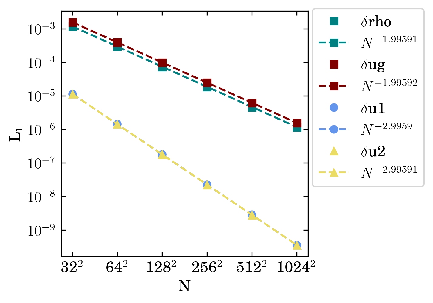
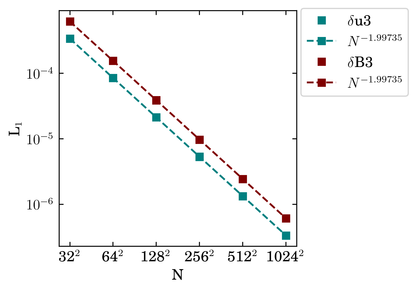
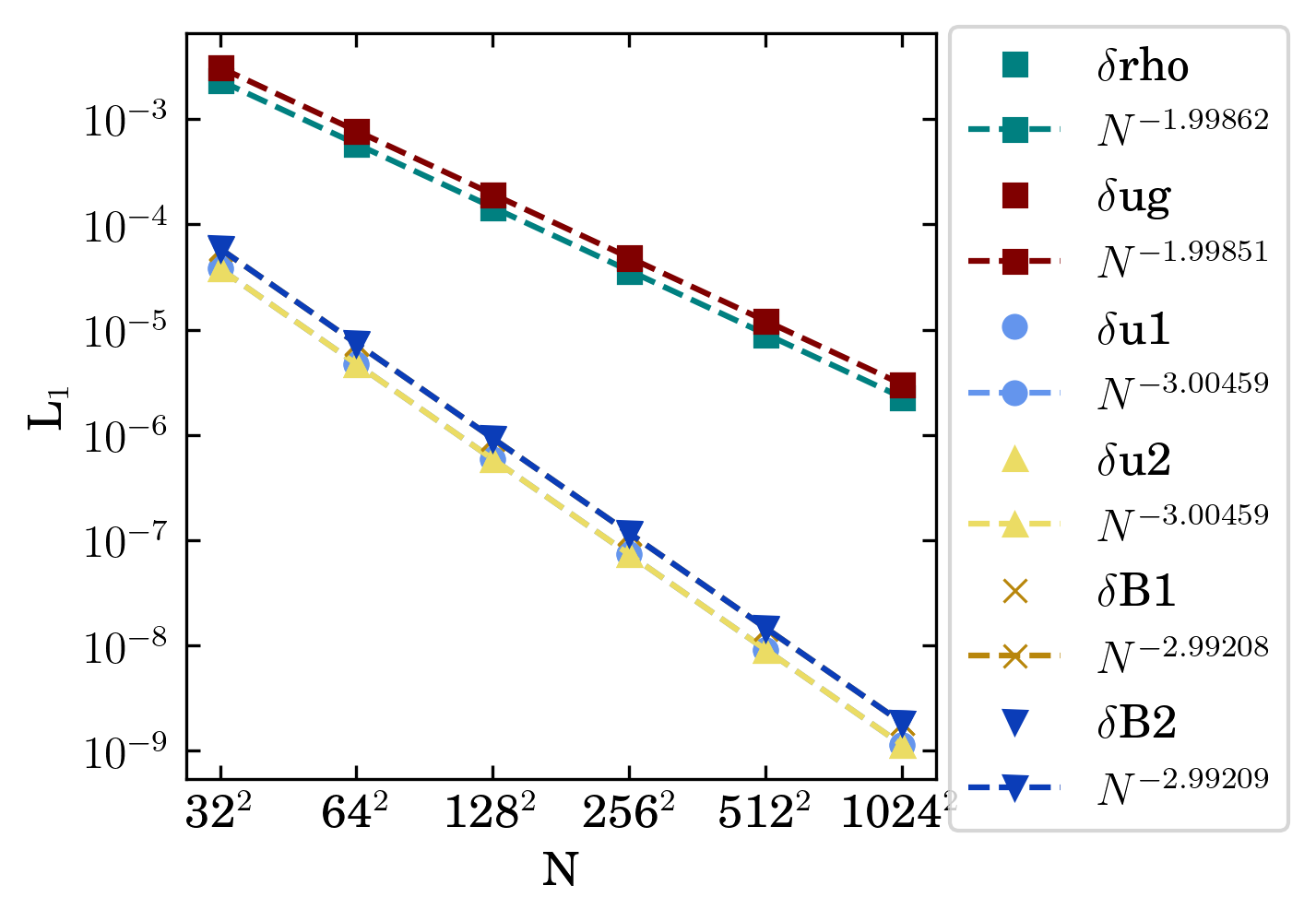
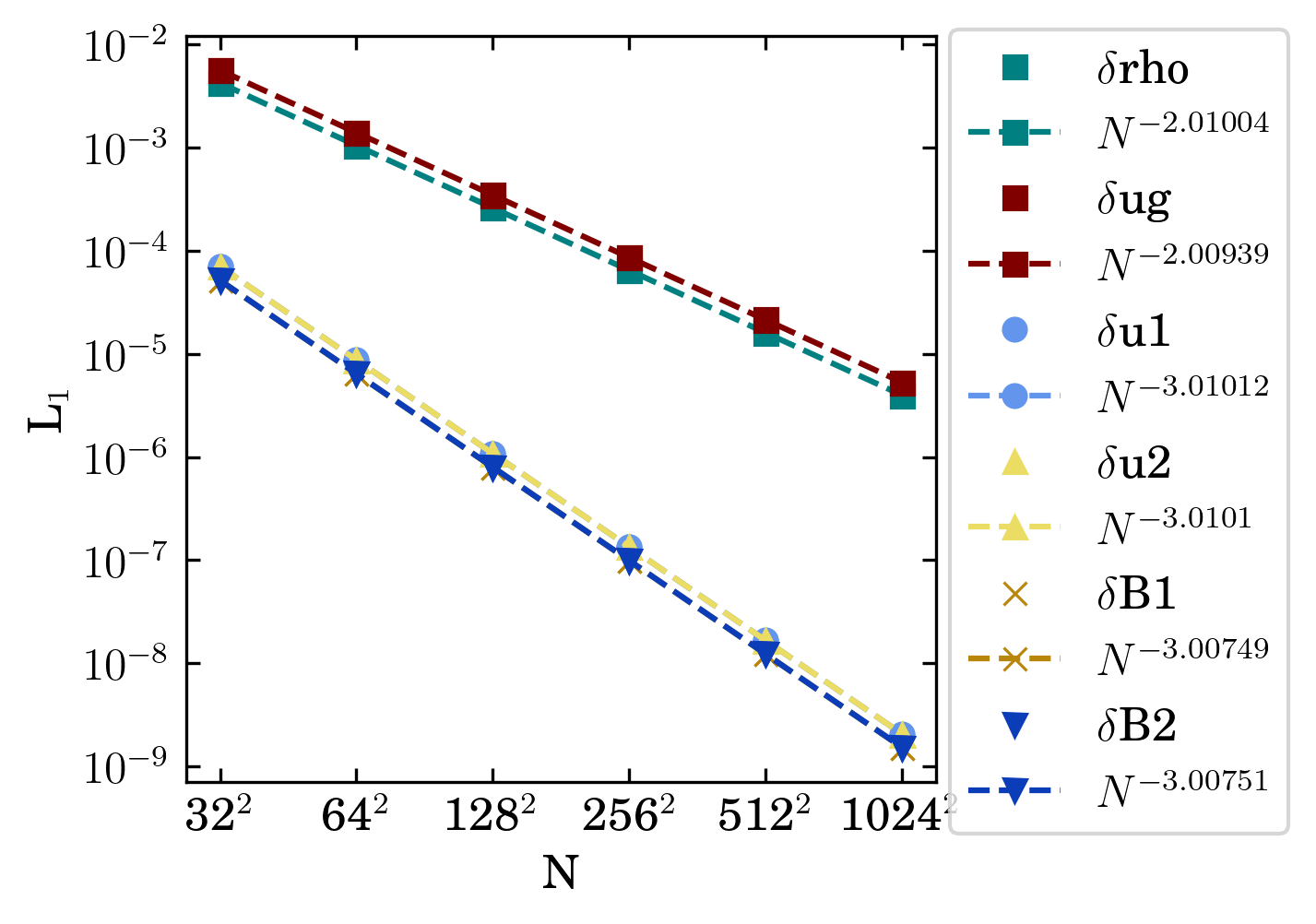
To measure the convergence of the tests presented here we use the $L_{1}$ norm scaled by the wave amplitude

$$L_{1}(q)=\frac{1}{kN^{2}}\sum_{i}\sum_{j}(q_{ij}-\hat{q}_{ij})$$ (61)

for quantity $q$, number of grid points along a dimension $N$, wave amplitude $k$, and solution $\hat{q}$. The tests are ran for one period such that the solution $\hat{q}$ is simply the initial condition. In Figures 1 – 4 we show $L_{1}$ convergence for relevant quantities for sound, Alfvén, fast, and slow magnetosonic waves, respectively. We consider resolutions $N^{2}$ = $32^{2}$, $64^{2}$, $128^{2}$, $512^{2}$, and $1024^{2}$. For all cases, we observe roughly at least the expected second order convergence.

Figure 1: $L_{1}$ convergence for the pure sound wave test. Shown is convergence for density (teal), internal energy (red), $v_{x}$ (light blue), and $v_{y}$ (yellow).

Figure 2: $L_{1}$ convergence for the pure Alfvén wave test. Shown is convergence for $v_{z}$ (teal) and $B_{z}$ (red).

Figure 3: $L_{1}$ convergence for the pure fast magnetosonic wave test. Shown is convergence for density (teal), internal energy (red), $v_{x}$ (light blue), $v_{y}$ (yellow), $B_{x}$ (gold x), and $B_{y}$ (dark blue triangles).

Figure 4: $L_{1}$ convergence for the pure slow magnetosonic wave test. Shown is convergence for density (teal), internal energy (red), $x$-velocity (light blue), and $y$-velocity (yellow) $B_{x}$ (gold x), and $B_{y}$ (dark blue triangles).

4.1.2 Nuclear EOS Shock Tube

Here we present a modification of the classic shock tube Riemann problem of Sod (1978). The test involves an initially stationary fluid with two states separated by a discontinuity. The initial state develops a shock propagating into the low density region, followed by a contact discontinuity, and a rarefaction wave propagating into the high density region. This test stresses a code’s ability to capture various hydrodynamic waves without introducing unphysical oscillations or viscosity.

We modify the traditional shock tube problem by the use of a realistic nuclear EOS (SFHo). This allows us to stress the code in regimes of astrophysical interest while simultaneously stressing the implementation of the nuclear EOS. For this test, our computational domain is $D=[0,300]$ km with an initial discontinuity located at $x=150$ km. The initial state $\mathbf{\mathcal{S}}$ = $(\rho,p,Y_{e})$ is given by

$$\mathbf{\mathcal{S}}=\\ \begin{cases}(10^{11},2.231\times 10^{31},0.3)&\text{left}\\ (0.25\times 10^{11},2.232\times 10^{30},0.5)&\text{right}\\ \end{cases}$$ (62)

for primitive density $\rho$ (in g cm^-3), pressure $p$ (in erg cm^-3) and electron fraction $Y_{e}$. The system is evolved until about $t=7.5$ms using 512 computational cells, WENO5-Z-AOAH reconstruction, and an HLL approximate Riemann solver. As an analytic solution does not exist with the use of a non-trivial EOS, we compare to a reference solution computed using thornado (Endeve et al., 2019; Pochik et al., 2021), a discontinuous Galerkin based GRRMHD code, computed using 16384 piecewise constant (P0) elements, 3rd order strong stability preserving explicit Runge Kutta time integration, an HLLC approximate Riemann solver (Toro et al., 1994). The thornado reference solution was computed using the same SFHo EOS. Figure 5 shows the density profile obtained with Phoebus (teal) compared to the thornado reference solution (black).

Figure 5: Numerical solution of the nuclear EOS shock tube at $t\approx 7.5$ms with Phoebus (teal) using 512 cells and piecewise linear reconstruction compared to a reference solution computed with thornado (black) using 16384 piecewise constant elements with 3rd order strong stability preserving Runge Kutta time integration.

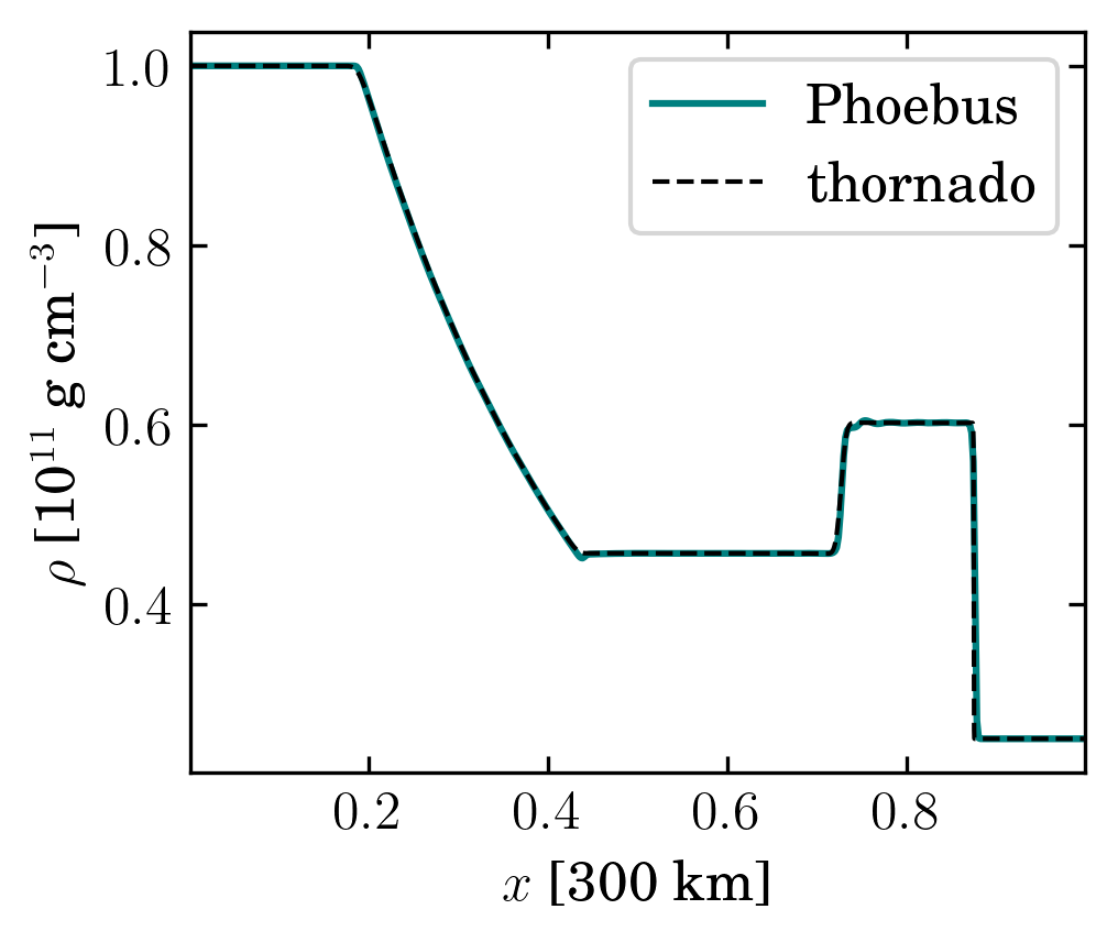
We see satisfactory agreement between the two codes.

4.1.3 Sedov–Taylor Blast Wave

Here we present the classic Sedov-Taylor blast wave (Sedov, 1946; Taylor, 1950). In this setup a large amount of energy is concentrated into a small volume, mocking an explosion and driving a spherical (or cylindrical in 2D) blast wave. This test stresses the scheme’s ability to handle shocks and spherical geometries.

We perform the test in 2D Cartesian coordinates, implying a cylindrical blast wave. An amount of energy $E=10^{-5}$ is deposited into all cells with $r<r_{\rm{init}}$ in an otherwise homogeneous medium. The medium has ambient density and pressure $\rho_{\rm{ambient}}=1.0$ and $p_{\rm{ambient}}=10^{-7}$. These initial conditions are chosen to ensure that Phoebus – a relativistic code – evolves in a manner consistent with the Newtonian self-similar solutions. We take $r_{\rm{init}}=0.1$ to set the volume of deposition. The computational domain is $D=[-1.0,1.0]\times[-1.0,1.0]$.

Figure 6: Top: 2D profile of density at $t=0.5$ with AMR levels overlaid. Bottom: Density along the $x$ coordinate at $y=0$ for Phoebus (teal crosses) compared to the self similar solution (black dashed). The vertical dashed line denotes the analytic shock position.

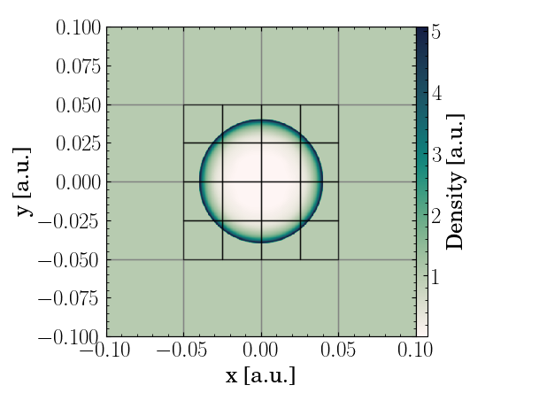
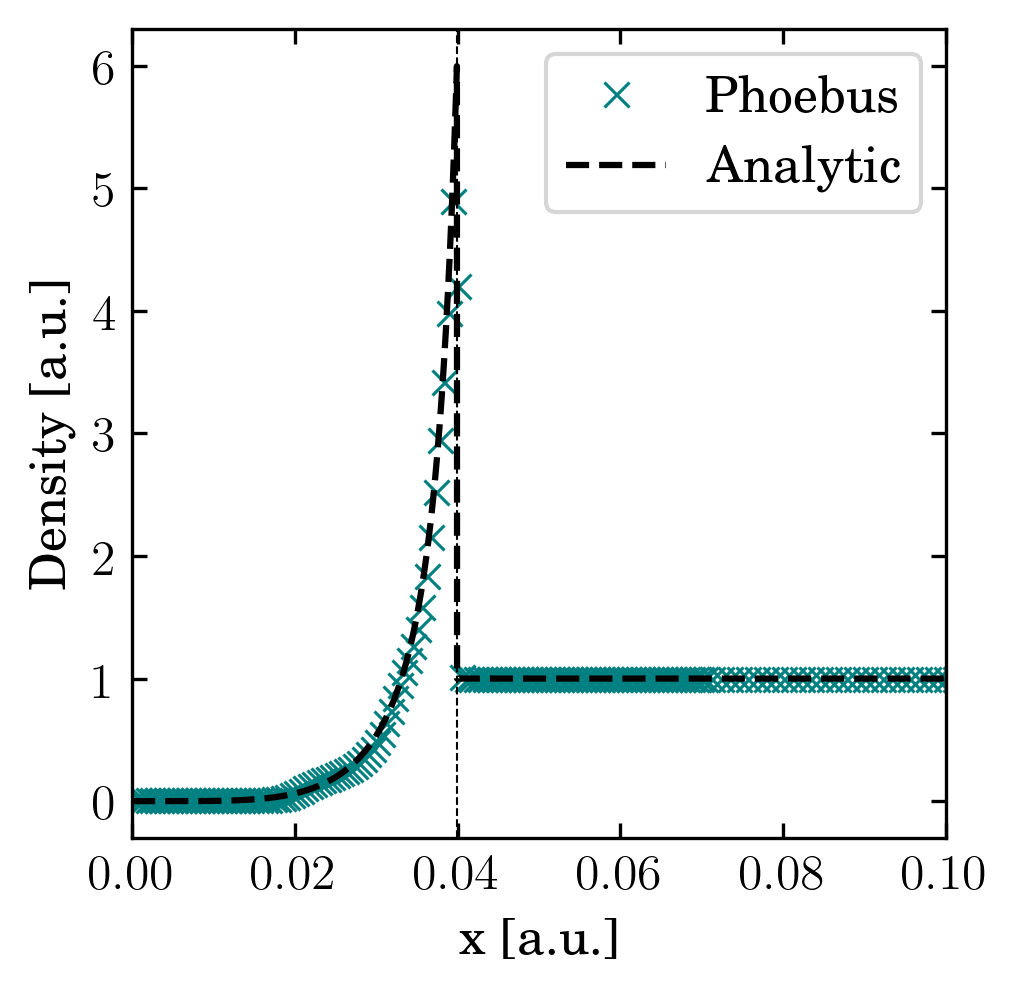
We perform the test with $N_{x}\times N_{y}=128\times 128$ computational cells. As an additional test of the AMR capabilities of Phoebus, we allow for up to five levels of mesh refinement. We evolve the system until $t=0.5$ Figure 6 shows the density profile from the blast wave (top). Overlaid on the profile are grid representative of the AMR refinement regions. We also show a 1D profile of density along the $x=y$ diagonal from the origin (bottom) compared to a semi-analytic self-similar solution .

4.1.4 Relativistic Blast Wave

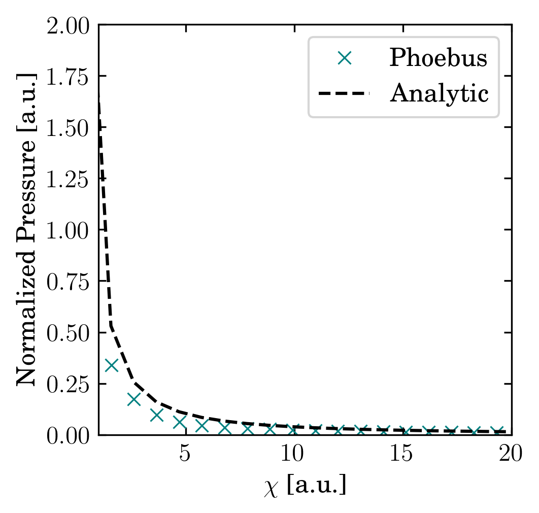
Here we present the Blandford-McKee blast wave (Blandford & McKee, 1976) – a relativistic complement to the non-relativistic Sedov-Taylor blast wave of the previous section. This test involves an ultra-relativistic shock wave characterized by Lorentz factor $W$ propagating into an ambient medium and stresses a scheme’s treatment of relativity and ability to capture relativistic shocks. For this test we initialize a shock wave with a Lortentz factor $W=10.0$ propagating into an ambient medium with $\rho_{0}=10^{-2}$ and $p_{0}=10^{-2}$. For this test we use an adiabatic index $\gamma=4/3$. We use 512 computational cells and allow for 2 levels of refinement. The domain is $r=[0,1]$ in spherical coordinates. Figure 7 shows the normalized post-shock pressure profile in the vicinity of the shock as a function of the similarity variable $\chi$, where $\chi=1.0$ is the shock position and $\chi>1$ is the post-shock region. For a shock in a uniform medium with no density gradient, the radial similarity variable is

$$\chi(r,t,W)=(1+2(m+1)W^{2})(1-r/t)$$ (63)

with $m=3$ for an impulsive, isolated blast wave. The normalized pressure similarity variable is then a power law

$$f(\chi)=\chi^{-17/12}.$$ (64)

Figure 7: Normalized pressure profile as a function of the self similar radial variable $\chi$ for Phoebus (teal) and analytic (black, dashed) solutions. The shock front is located at $\chi=1.0$ and $\chi>1.0$ is the post-shock region.

4.2 Tracer Particles

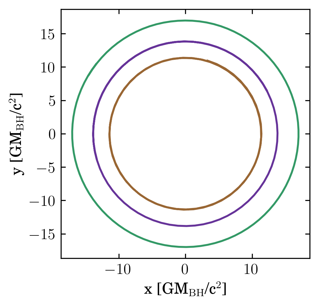
Here we test the tracer particles infrastructure as described in Section 3.5. To stress the coupling to both the fluid and the spacetime, we model a 3D accretion disk in near hydrostatic equilibrium around a black hole. We adopt the torus configuration of Fishbone & Moncrief (1976). We initialize a torus of constant entropy and specific angular momentum with no initial magnetic field around a Kerr black hole. We assume an ideal gas equation of state for this test. The test is run in three spatial dimensions with $N_{r}\times N_{\theta}\times N_{\phi}$ = $128\times 128\times 128$ cells and 10⁴ tracer particles. The system is evolved until $t=2000GM_{BH}/c^{3}$. Tracer particles are sampled uniformly in volume on the initial condition.

With no initial magnetic field we will not develop the magnetorotational instability (MRI) responsible for driving accretion on to the central compact object. Instead, the disk – and by extension, tracer particles – will orbit the black hole, until other hydrodynamic instabilities arise at later times. Figure 8 shows the trajectories of three select tracer particles throughout the evolution projected into the $xy-$plane. The innermost tracer covers several orbits through the evolution while the outermost covers slightly more than one. The tracer particles show the expected behavior, orbiting the central black hole (located here at $x=y=0$). However, as the tracer particle integration is not symplectic, we do not expect, or observe, perfectly closed orbits. Future work includes the implementation of a symplectic integrator for tracer particle advection.

Figure 8: Paths of three select tracer particles evolved in the equilibrium disk.

4.3 Transport

In this section we present a suite of tests from Miller et al. (2019) stressing the radiation transport schemes. Unless otherwise noted, all tests use Monte Carlo transport.

4.3.1 Artificial Neutrino Cooling

We test the coupling of neutrinos to matter in a simplified context. We construct a homogeneous, isotropic gas cooled by only either electron neutrinos or antineutrinos using a simplified “tophat” emissivity

$$j_{\nu,f}=Cy_{f}\left(Y_{e}\right)\chi\left(\nu_{\mathrm{min}},\nu_{\mathrm{max}}\right),$$ (65)

where $C$ is a constant ensuring correct units,

$$\chi(\nu_{\mathrm{min}},\nu_{\mathrm{max}})=\begin{cases}1&\text{for}\ \nu_{\mathrm{min}}\leq\nu\leq\nu_{\mathrm{max}}\\ 0&\text{otherwise}\end{cases}$$ (66)

and

$$y_{f}\left(Y_{e}\right)=\begin{cases}2Y_{e}&\text{for}\ \nu_{e}\text{emission}\\ 1-2Y_{e}&\text{for}\ \bar{\nu}_{e}\text{emission}\\ 0&\text{otherwise}.\end{cases}$$ (67)

The gas is at a uniform density of $10^{6}$ g cm^-1 with an internal energy density of $10^{20}$ erg cm^-3 and electron fraction

$$Y_{e}\left(t=0\right)=\begin{cases}\frac{1}{2}&\text{for}\ \nu_{e}\\ 0&\text{for}\ \bar{\nu}_{e}.\\ \end{cases}$$ (68)

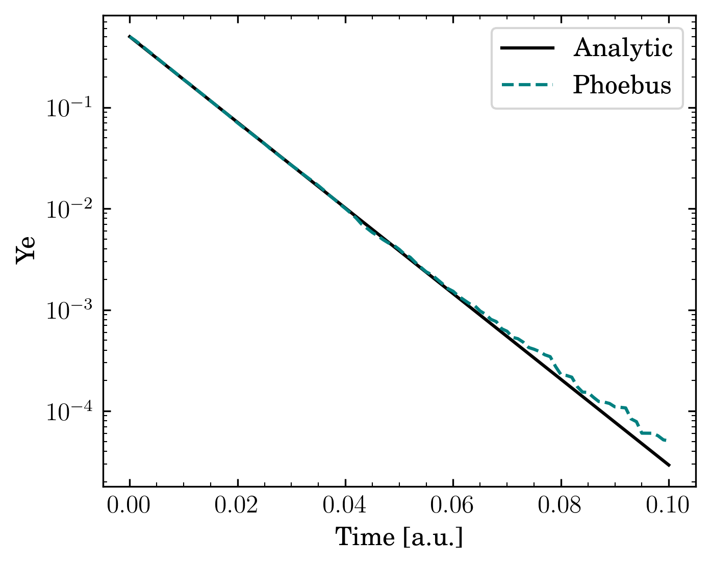
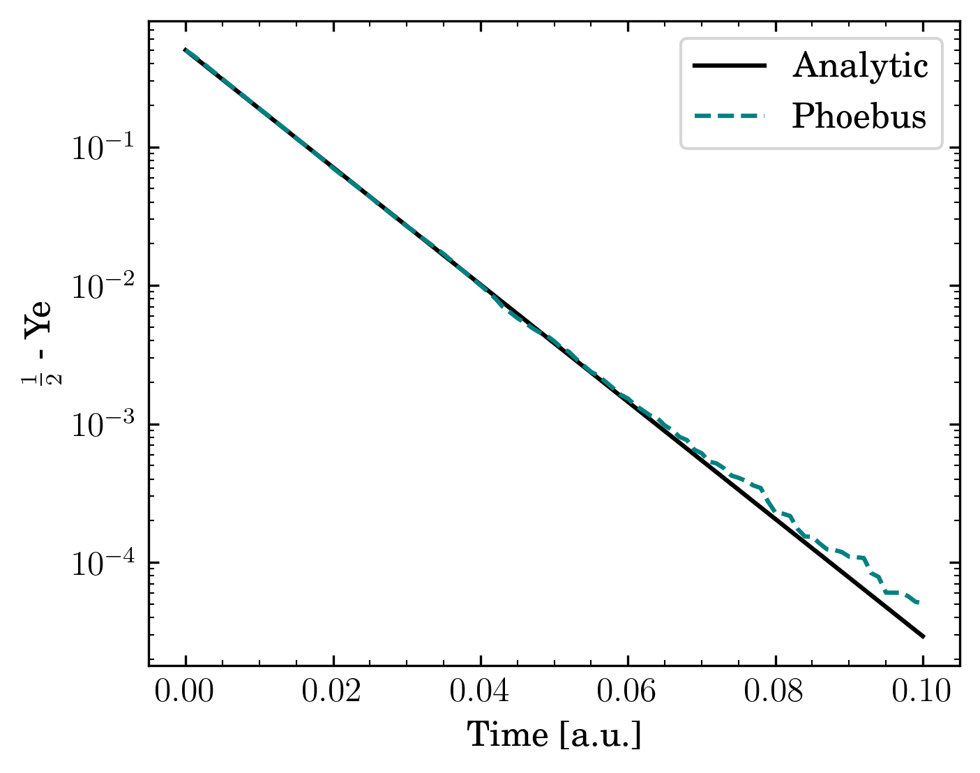
In this simplified setting, the electron fraction evolution has an analytic solution (Miller et al., 2019)

$$Y_{e}\left(t\right)=\begin{cases}-\frac{1}{2}e^{-2A_{C}t}&\text{for}\ \nu_{e}\\ \frac{1}{2}\left(1-e^{-2A_{C}t}\right)&\text{for}\ \bar{\nu}_{e}\\ \end{cases}$$ (69)

where $A_{C}=\frac{m_{p}}{h\rho}C\mathrm{ln}(\frac{\nu_{\mathrm{max}}}{\nu_{\mathrm{min}}})$ for proton mass $m_{p}$, Planck’s constant $h$, and density $\rho$.

This setup was run until $t=0.1$ (in arbitrary code units) using 100 frequency bins and only 16 Monte Carlo packets. Figure 9 (10) shows the electron fraction as a function of time for a gas cooled by electron neutrinos (antineutrinos). Agreement with the analytic solution is very good, with very small deviations at late times due to Monte Carlo noise.

Figure 9: Electron fraction for a homogeneous isotropic gas cooling by electron neutrinos. The solid line is the analytic solution and the dashed line is the Phoebus solution.

Figure 10: Electron fraction for a homogeneous isotropic gas cooling by electron antineutrinos. The solid line is the analytic solution and the dashed line is the Phoebus solution.

4.3.2 Neutrino-Driven Wind Setup

The tests of the previous section use artificial neutrino emissivities. While useful for comparison with a known analytic solution, they do not represent physically realistic or interesting settings. In this section we consider a setting of astrophysical interest and compare to the supernova code fornax (Skinner et al., 2018). fornax uses notably different methods from Phoebus, with Phoebus being fully general relativistic and fornax having an approximate treatment for gravity. fornax treats radiation using a multi-group moment based approach with the M1 closure (Shibata et al., 2011; Cardall et al., 2013) whereas Phoebus uses a Monte Carlo approach in addition to the other methods outlined in Section 3.

To facilitate comparison between codes and to test Phoebus in astrophysically motivated settings, we consider a homogeneous and isotropic gas at rest on a periodic domain in Minkowski space. Phoebus and fornax both use the same commonly adopted SFHo nuclear matter equation of state (Steiner et al., 2013b) and opacities. We consider the following initial state, motivated by conditions realized in neutrino-driven outflow

$$\begin{split}\rho_{0}&=10^{9}\ \text{g cm}^{-3}\\ T&=2.5\ \text{MeV}\\ Y_{e}&=0.1.\end{split}$$ (70)

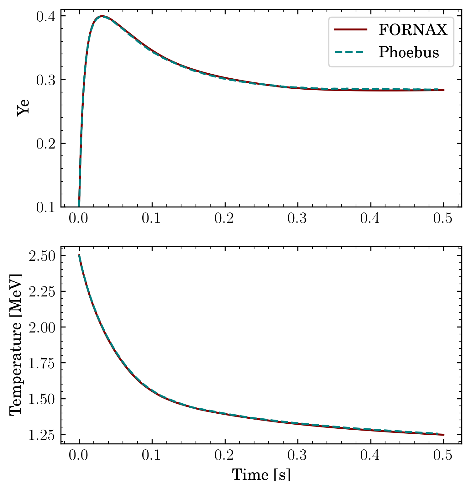
The problem is evolved for 0.5 seconds assuming no initial radiation. Both codes are run with 200 frequency groups ranging from 1 to 300 MeV. Phoebus is run with a target number of $10^{5}$ Monte Carlo packets. Both codes include three neutrino flavors: $\nu_{e}$, $\bar{\nu}_{e}$, and $\nu_{x}$, where $\nu_{x}$ is a representative “heavy” neutrino combining the $\mu$ – $\tau$ neutrinos and antineutrinos.

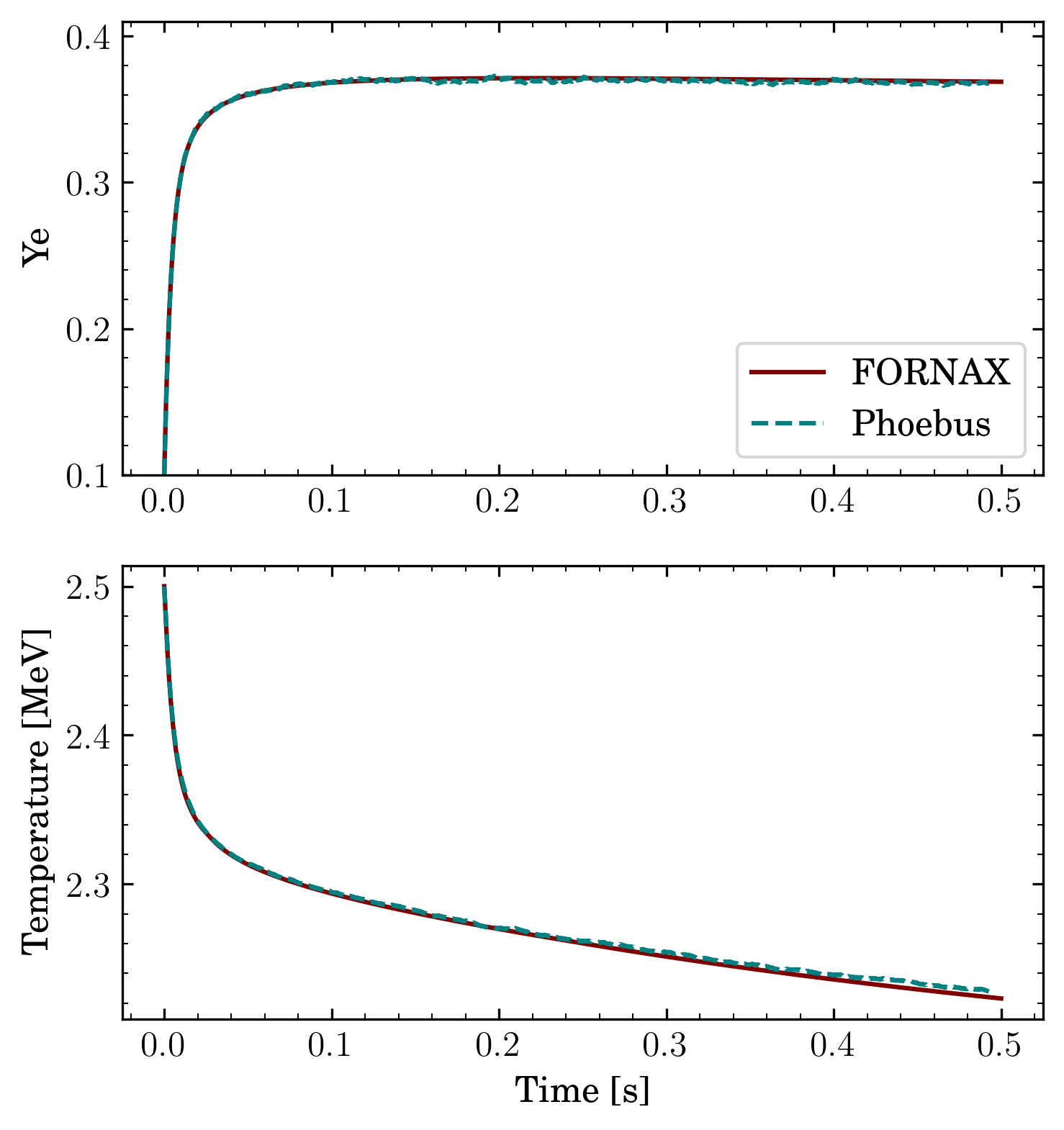
We consider first the case of pure cooling by neutrinos, disabling absorption opacities. Electron fraction and temperature evolution for both Phoebus (blue dashed line) and fornax (red solid line) are shown in Figure 11. Phoebus displays the expected rapid cooling behavior and agrees very well with the fornax solution.

Next we consider the case of emission and absorption of neutrinos, allowing the radiation and gas to come to thermal equilibrium. We show electron fraction and temperature evolution for both Phoebus (blue dashed line) and fornax (red solid line) in Figure 12. As with the previous test, the electron fraction rapidly, but cooling is slowed due to absorption of neutrinos. Again we see good agreement between the codes with small Monte Carlo noise in the equilibrium electron fraction.

Figure 11: Electron fraction (top) and temperature (bottom) for the optically thin cooling comparison between Phoebus (dashed line) and fornax (solid line).

Figure 12: Electron fraction (top) and temperature (bottom) for the thermal equilibrium comparison between Phoebus (dashed line) and fornax (solid line).

4.3.3 Two Dimensional Lepton Transport

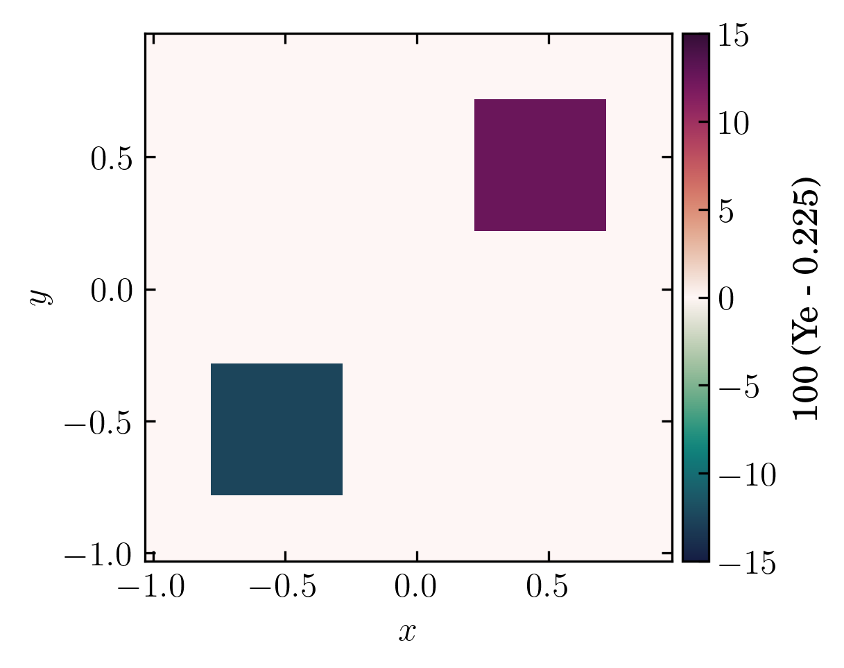
Neutrinos, unlike photon radiation, can exchange energy, momentum, as well as lepton number with the matter field. This motivates an accurate treatment of neutrino transport, as the matter composition can influence the resulting nucleosynthesis, among other things. We test the ability for Phoebus to capture this lepton number exchange by considering a two-dimensional test problem. We let our domain be a periodic box with $(x,y)\in[-1,1]^{2}$. The initial state is a gas with constant density and temperature

$$\begin{split}\rho_{0}&=10^{10}\ \text{g cm}^{-3}\\ T&=2.5\ \text{MeV}\end{split}$$ (71)

and electron fraction defined by

$$Y_{e}=\begin{cases}0.100&\text{for}\ (x,y)\in[-0.75,-0.25]^{2}\\ 0.350&\text{for}\ (x,y)\in[0.25,0.75]^{2}\\ 0.225&\text{otherwise.}\end{cases}$$ (72)

This describes a region of stellar material with an electron fraction “hot spot” and “cold spot”. We do not allow the gas to evolve due to pressure gradients, allowing instead only interaction with the radiation field in order to highlight the impact of lepton number transport. We use 2.5$\times 10^{5}$ Monte Carlo packets with 200 frequency bins distributed from roughly 100 keV to 300 MeV. We include three flavors of neutrinos.

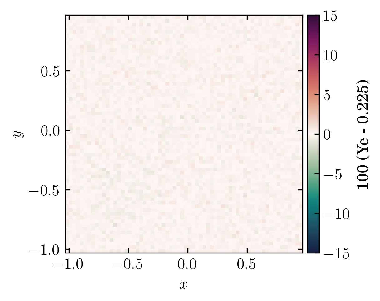
Figure 13 shows the initial condition (left) and state at $t\approx 10$ms (right). We observe the expected behavior where the neutrinos equilibrate with the matter, with the final state being perturbed from the initial state.

Figure 13: Left: Initial condition for the lepton equilibration problem. Right: The system after about 10 ms. The neutrino radiation field brings the electron fraction field into equilibrium.

4.4 Gravity

4.4.1 Homologous Collapse

Here we test the general relativistic gravity solver in Phoebus with the homologous collapse problem (Goldreich & Weber, 1980). For this test we use the spherically symmetric monopole gravity solver of Section 2.3.1. This problem serves to test the coupling between gravity and hydrodyamics in a setting relevant to CCSNe. It involves a homologously collapsing core ($\mathbf{u}\propto\mathbf{r}$) with mass $M$ and size $R$. The system is described by the continuity equation, Euler’s equation, and Poisson’s equation:

$$\frac{\partial\rho}{\partial t}+\bm{\nabla}\cdot(\rho\bm{u})=0,$$ (73)

$$\frac{\partial\bm{u}}{\partial t}+\bm{\nabla}\bigg{(}\frac{|\bm{u}|^{2}}{2}\bigg{)}+(\bm{\nabla}\times\bm{u})\times\bm{u}+\bm{\nabla}h+\bm{\nabla}\Phi=0,$$ (74)

$$\nabla^{2}\Phi-4\pi G\rho=0,$$ (75)

where $\bm{u}$ is the fluid velocity, $\Phi$ is the gravitational potential, $h$ is the heat function $h=\int\frac{dp}{\rho}=4\kappa\rho^{1/3}$. If one assumes vorticity-free flow and an analytic, $n=3$, $\gamma=4/3$ polytropic equation of state, one can find a semi-analytic solutions to the system of equations (Equations (73) - (75)). In this approximation, the fluid velocity, density, and the gravitational potential are given by:

$$\bm{u}=\dot{a}\bm{r}\,,$$ (76)

$$\rho=\bigg{(}\frac{\kappa}{\pi G}\bigg{)}^{3/2}a^{-3}f^{3}\,,$$ (77)

$$\Phi=\frac{\Psi}{c_{s}^{-2}}=\bigg{(}\frac{\gamma P_{c}}{\rho_{c}}\bigg{)}\Psi=\frac{4}{3}\bigg{(}\frac{\kappa^{3}}{\pi G}\bigg{)}^{1/2}\frac{\Psi}{a}\,,$$ (78)

where $a$ is Jean’s length and is found to be

$$a(t)=(6\lambda)^{1/3}\bigg{(}\frac{\kappa^{3}}{\pi G}\bigg{)}^{1/6}[t+t_{0}]^{2/3}\,,$$ (79)

where $\lambda$ a constant determined by initial conditions. $f$ is a normalization function for the density and is determined by the following differential equation:

$$\frac{1}{r^{2}}\frac{\partial}{\partial r}\bigg{(}r^{2}\frac{\partial f}{\partial r}\bigg{)}+f^{3}=\lambda$$ (80)

Finally, $\Psi$ can be found using

$$\Psi=\frac{\lambda}{2}r^{2}-3f$$ (81)

We incorporate the homologous collapse test problem in Phoebus and compare results with the semi-analytic solutions of Equations (79) - (81).

Figure 14: Density profile of the homologous collapsing star with mass $M=1.4M_{\odot}$ and size $R=3000\rm km$ at $t=0.12\rm s$ after the start of the collapse.

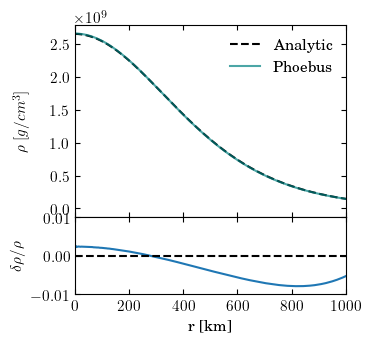
Figure 14 shows the comparison of the density profiles between the simulation and analytic solution. We simulate one-dimensional homologous collapse of a star with mass $M=1.4M_{\odot}$ and size $R=3000\rm km$. The number of zones in $x$ direction is $10000$. The analytic solution of Goldreich & Weber (1980) uses Newtonian approximation for gravity, while the simulation in Phoebus is solved in the monopole approximation for GR. This difference causes a different behavior in the time evolution between the simulation and analytic solution; for example, central density changes faster in the simulation. To compare the simulation and analytic results, we choose some time moment on the simulation, $t=0.12\rm s$ and find corresponding Jeans length from the simulation. Then solve the analytic equations given this value of Jeans length. As a result, the density profile on the simulation matches well with the density profile obtained from analytic solutions; the variation is $\delta\rho/\rho_{\rm analytic}\leq 1\%$ .

5 Performance

In this section we briefly explore the parallel performance of Phoebus. We focus on the weak scaling behavior of Phoebus on the new LANL supercomputing resource Venado. Venado deploys new NVIDIA Grace-Hopper H100 nodes. Weak scaling demonstrates a code’s ability to effectively use large resources. We run a 3D Sedov–Taylor blast wave beginning with a 128³ uniform grid and a single meshblock on a single H100 node (4 GPUs). We cyclically double the resolution in $x^{1}$, $x^{2}$, and $x^{3}$ while doubling the number of GPUs. Performance is measured in zone-cycles per second, or the number of cells updated in a single wall clock second. Figure 15 shows the weak scaling performance (top) and efficiency (bottom).

Figure 15: Weak scaling performance (top) and efficiency (bottom) on Venado H100s.

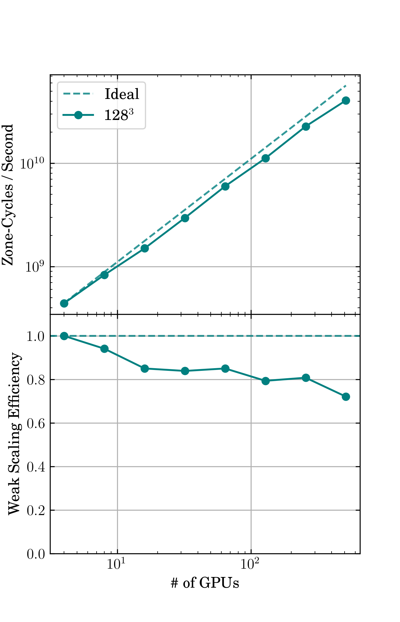
We observe just below 80$\%$ weak scaling efficiently on 512 H100s. At this scale we reach a few 10¹⁰ zone-cycles per second. While the performance is quite good it is poorer than has been observed on other parthenon  codes (Grete et al., 2022). There are a number of near-future modifications planned to address this and achieve even better weak scaling.

6 Discussion and Conclusions

In this paper, we have introduced Phoebus, a new code for general relativistic radiation magnetohydrodynamic simulations of astrophysical phenomena, Phoebus.

Phoebus models general relativistic neutrino radiation magnetohydrodynamics. General relativistic hydrodynamics are incorporated with the Valencia formulation. MHD is incorporated using a cell centered constrained transport treatment and discretized with a finite volumes approach. Neutrino transport is incorporated using a Monte Carlo approach as well as a gray two moment scheme. Gravity is incorporated through analytic and tabular spacetimes and a novel monopole solver for core-collapse supernovae. The physics capabilities of Phoebus have been demonstrated through a suite of tests stressing individual physics implementations as well as the couplings between them. We have demonstrated the weak scaling efficiency of Phoebus on NVIDIA H100s.

Phoebus is developed on top of, and supported by, a large, open source ecosystem. Phoebus supports block based adaptive mesh refinement via the parthenon  framework and achieves performance portability with the kokkos  hardware agnostic library. Flexible, portable equations of state are supported through singularity-eos . Spiner enables performance portable storage and interpolation of tabular data, such as for equations of state and opacities (Miller et al., 2022). This open source ecosystem providing performance portability allows Phoebus developers to focus primarily on physics and numerics and ensures the longevity of the project.

There are a number of improvements planned for the near future that will greatly bolster the capabilities of Phoebus. Of note: we will adopt a proper face-centered-fields approach to MHD constrained transport. Moment based neutrino transport will be upgraded to allow for frequency dependent evolution. The finite volume discretization for hydrodynamics will be upgraded to be formally 4th order. Modifications to further improve the scaling performance of Phoebus are planned. Finally, a full dynamic GR solver is in prep with a separate methods paper forthcoming.

In the interest of open science, to provide a tool for the community, and allow for full reproducability, Phoebus and all parts of its ecosystem are open source. Phoebus is publicly available on GitHub. We welcome, and look forward to, contributions, engagement, feedback, and scientific productivity from the greater community.

Appendix A Time-derivatives of the monopole metric

To compute the Christoffel symbols, one needs derivatives of the metric in both space and time. The spatial derivatives are straightforward: with $a$, $K$, $\alpha$, and $\beta^{r}$ known, simply differentiate with respect to $r$. The time derivatives are more subtle. We use the Einstein evolution equations to derive them.

First we note that ADM evolution equation for the metric reduces to the following in spherical symmetry:

$$\partial_{t}g_{\mu\nu} = \beta^{\sigma}\partial_{\sigma}g_{\mu\nu}+g_{\sigma\mu}\partial_{\nu}\beta^{\sigma}+g_{\sigma\nu}\partial_{\mu}\beta^{\sigma}-2\alpha K_{\mu\nu}$$ (A1)

$$= \beta^{r}\partial_{r}g_{\mu\nu}+g_{r\mu}\partial_{\nu}\beta^{r}+g_{r\nu}\partial_{\mu}\beta^{r}-2\alpha K_{\mu\nu}.$$

The $rr$-component of equation (A1) yields an equation for the derivative of $a$:

$$\partial_{t}g_{rr} = \beta^{r}\partial_{r}(a^{2})+2g_{rr}\partial_{r}\beta^{r}-2\alpha K_{rr}$$ (A2)

$$= 2aa^{\prime}\beta^{r}+2a^{2}\partial_{r}\beta^{r}-2\alpha a^{2}K^{r}_{r}$$

$$= 2a(a^{\prime}\beta^{r}+a(\beta^{r})^{\prime}-\alpha aK^{r}_{r}).$$

$$= -2\alpha\partial_{t}\alpha+2a(\beta^{r})^{2}\partial_{t}a-ra^{2}\beta^{r}(\alpha\partial_{t}K^{r}_{r}+K^{r}_{r}\partial_{t}\alpha)$$

But note that, from the line element (Eq 15)

$$\partial_{t}g_{rr}=\partial_{t}a^{2}=2a\partial_{t}a,$$

so

$$\partial_{t}a=a^{\prime}\beta^{r}+a(\beta^{r})^{\prime}-\alpha aK^{r}_{r}.$$ (A3)

The lapse proceeds similarly. We start with the fact that

$$g_{tt} = -\alpha^{2}+\beta^{2}$$

$$= -\alpha^{2}+a^{2}(\beta^{r})^{2}$$

$$\Rightarrow\partial_{t}g_{tt} - -2\alpha\partial_{t}\alpha+2a(\beta^{r})^{2}\partial_{t}a+2a^{2}\beta^{r}\partial_{t}\beta^{r}$$

$$= -2\alpha\partial_{t}\alpha+2a(\beta^{r})^{2}\partial_{t}a+2a^{2}\beta^{r}\left[-\frac{1}{2}r(\alpha\partial_{t}K^{r}_{r}+K^{r}_{r}\partial_{t}\alpha)\right]$$

We then proceed to apply the metric evolution equation (A1) on $g_{tt}$:

$$\partial_{t}g_{tt} = -\beta^{r}\partial_{r}g_{tt}+2g_{rt}\partial_{t}\beta^{r}-2\alpha K_{tt}$$ (A4)

$$= \beta^{r}\partial_{r}g_{tt}+2g_{rt}\left[-\frac{1}{2}r(\alpha\partial_{t}K^{r}_{r}+K^{r}_{r}\partial_{t}\alpha)\right]-2\alpha K_{tt}$$

$$= \beta^{r}\partial_{t}g_{tt}-ra^{2}\beta^{r}(\alpha\partial_{t}K^{r}_{r}+K^{r}_{r}\partial_{t}\alpha)-2\alpha a^{2}K^{r}_{r}(\beta^{r})^{2}$$

We now combine equations (A) and (A4). The

$$ra^{2}\beta^{r}(\alpha\partial_{t}K^{r}_{r}+K^{r}_{r}\partial_{t}\alpha)$$

term cancels and we find that

$$-2\alpha\partial_{t}\alpha+2a(\beta^{r})^{2}\partial_{t}a=\beta^{r}\partial_{r}g_{tt}-2a^{2}\alpha K^{r}_{r}(\beta^{r})^{2}$$

$$\Rightarrow\partial_{t}\alpha = \frac{a}{\alpha}(\beta^{r})^{2}\dot{a}+a^{2}K^{r}_{r}(\beta^{r})^{2}-\frac{\beta^{r}}{\alpha}\partial_{r}g_{tt}$$ (A5)

$$= \frac{a}{\alpha}(\beta^{r})^{2}\dot{a}+a^{2}K^{r}_{r}(\beta^{r})^{2}-\frac{\beta^{r}}{\alpha}\left[-2\alpha\partial_{r}\alpha+2\alpha(\beta^{r})^{2}\partial_{r}a+2a^{2}\beta^{r}\partial_{r}\beta^{r}\right]$$

$$= \frac{a}{\alpha}(\beta^{r})^{2}\dot{a}+a^{2}K^{r}_{r}(\beta^{r})^{2}+2\beta^{r}\alpha^{\prime}-2(\beta^{r})^{3}a^{\prime}-2a^{2}\frac{(\beta^{r})^{2}}{\alpha}\partial_{r}\beta^{r}$$

$$= \beta^{r}\left[\frac{a\beta^{r}\dot{a}}{\alpha}+a^{2}K^{r}_{r}\beta^{r}+2a^{\prime}(1-(\beta^{r})^{2})-2\frac{a^{2}\beta^{r}}{\alpha}\partial_{r}\beta^{r}\right]$$

Finally, we reach the time derivative of $\beta$. To calculate it, we require the time derivative of $K^{r}_{r}$, which comes from the ADM evolution equation for the extrinsic curvature. We begin with the following relation:

$$K^{i}_{j} = \gamma^{ik}K_{kj}$$

$$\Rightarrow(\partial_{t}-\mathcal{L}_{\beta})K^{i}_{j} = \gamma^{ik}(\partial_{t}-\mathcal{L}_{\beta})K_{kj}+K_{kj}(\partial_{t}-\mathcal{L}_{\beta})\gamma^{ik}$$ (A6)

$$= \gamma^{ik}(\partial_{t}-\mathcal{L}_{\beta})K_{kj}-2\alpha K^{i}_{k}K^{k}_{j},$$

We thus have

$$(\partial_{t}-\mathcal{L}_{\beta})K^{i}_{j} = -D^{i}D_{j}\alpha+\alpha\left[{}^{(3)}R^{i}_{j}+KK^{i}_{j}-2K^{i}_{k}K^{k}_{j}\right]+4\pi\alpha\left[\delta^{i}_{j}(S-\rho)-2S^{i}_{j}\right]-2\alpha K^{i}_{k}K^{k}_{j}$$

$$= -D^{i}D_{j}\alpha+\alpha\left[{}^{(3)}R^{i}_{j}-4K^{i}_{k}K^{k}_{j}\right]+4\pi\alpha\left[\delta^{i}_{j}(S-\rho)-2S^{i}_{j}\right]$$

$$\Rightarrow\partial_{t}K^{i}_{j} = \beta^{k}\partial_{k}K^{i}_{j}-K^{k}_{j}\partial_{k}\beta^{i}+K^{i}_{k}\partial_{j}\beta^{k}-D^{i}D_{j}\alpha+\alpha\left[{}^{(3)}R^{i}_{j}-4K^{i}_{k}K^{k}_{j}\right]+4\pi\alpha\left[\delta^{i}_{j}(S-\rho)-2S^{i}_{j}\right].$$

When we specialize to $i=j=r$, this becomes

$$\partial_{t}K^{r}_{r} = \beta^{r}\partial_{r}K^{r}_{r}-K^{r}_{r}\partial_{r}\beta^{r}+K^{r}_{r}\partial_{r}\beta 2-D^{r}D_{r}\alpha+\alpha\left[{}^{(3)}R^{r}_{r}-4(K^{r}_{r})^{2}\right]+4\pi\alpha\left[S-\rho-2S^{r}_{r}\right]$$ (A7)

$$= \beta^{r}\partial_{r}K^{r}_{r}-D^{r}D_{r}\alpha+\alpha[^{(3)}R^{r}_{r}-4(K^{r}_{r})^{2}]-4\pi\alpha(S-\rho-2S^{r}_{r}).$$

Given metric ansatz (15), we have

$${}^{(3)}R_{rr} = \frac{2}{abr}\left\{a^{\prime}[(b+rb^{\prime})-arb^{\prime\prime}]-2ab^{\prime}\right\}$$

$$= \frac{2}{ar}a^{\prime}$$

$$\Rightarrow^{(3)}R^{r}_{r} = \frac{2}{a^{3}r}a^{\prime}$$ (A8)

and since $\alpha$ is a scalar,

$$D^{i}D_{j}\alpha = D^{i}\partial_{j}\alpha$$

$$= \gamma^{ik}D_{k}\partial_{j}\alpha$$

$$= \gamma^{ik}(\partial_{k}\partial_{j}\alpha-^{(3)}\Gamma^{l}_{kj}\partial_{l}\alpha)$$

$$= \gamma^{ik}(\partial_{k}\partial_{j}\alpha-^{(3)}\Gamma^{r}_{kj}\partial_{r}\alpha)\text{ because only non-trivial derivatives are in }r$$

$$\Rightarrow D^{r}D_{r}\alpha = \gamma^{rk}(\partial_{k}\partial_{r}\alpha-^{(3)}\Gamma^{r}_{kr}\partial_{r}\alpha)$$ (A9)

$$= \gamma^{rr}(\partial_{r}^{2}\alpha-^{(3)}\Gamma^{r}_{rr}\alpha)\text{ because }\gamma\text{ is diagonal}$$

$$= \frac{1}{a^{2}}\left(\partial_{r}^{2}\alpha-\frac{a^{\prime}}{a}\partial_{r}\alpha\right)$$

$$= \frac{1}{a^{2}}\partial_{r}^{2}\alpha-\frac{a^{\prime}}{a^{3}}\partial_{r}\alpha$$

Which implies

$$\partial_{t}K^{r}_{r}=\beta^{r}\partial_{r}K^{r}_{r}-\frac{1}{a^{2}}\partial_{r}^{2}\alpha+\frac{a^{\prime}}{a^{3}}\partial_{r}\alpha+\alpha\left[\frac{2}{a^{3}r}a^{\prime}-4(K^{r}_{r})^{2}\right]+4\pi\alpha\left[S-\rho-2S^{r}_{r}\right]$$ (A10)

which provides, along with equation (21) and the chain rule, a solution for the time-derivative of the shift.

We note that $S^{r}_{r}$ can be computed simply in spherical symmetry from $S$ via the following reasoning. In spherical symmetry, the spatial stress tensor must be diagonal. Moreover, the diagonal components must be

$$S^{\theta}_{\theta}=S^{\phi}_{\phi}=P+\frac{1}{2}b^{2}.$$

Therefore,

$$S^{r}_{r} = S-S^{\theta}_{\theta}-S^{\phi}_{\phi}$$ (A11)

$$= S-2(P+\frac{1}{2}b^{2})$$

$$= \tau+D+P-(\rho+u)-P^{i}_{\mu}P_{i}^{\nu}b^{\mu}b_{\nu}$$

We use this relation.

Appendix B Our novel WENO5-Z-AOAH scheme

Consider a grid of cells of equal width $\Delta x$ with centers at positions $x_{i}$ for $i=0,1,\ldots,N$ for some $N\geq 5$. A function $f(x)$ is known at cell centers, with values $f_{i}=f(x_{i})$. For some index $j$ we wish to reconstruct the value of $f$ at the cell face between centers $x_{j}$ and $x_{j+1}$, i.e., at $x_{j+1/2}$. Ideally, if $f$ is a smooth function, this reconstruction should be high-order, such that the truncation error is small. However, if $f$ is not smooth, then the reconstruction should be robust and minimize the Gibbs oscillations that emerge from high-order representations of non-smooth functions (Wilbraham, 1848; Gibbs, 1898).

The WENO family of methods, first described by Shu (2009) seek to solve the above-described problem. For smooth problems, WENO constructs a high-order interpolant from the linear combination of several lower-order interpolants. For example, a fifth-order interpolant, $P^{(5)}(x_{j+1/2})$ evaluated at $x_{j+1/2}$ may be constructed from the linear combination of three third-order interpolants $P^{(3)}_{k}$, $k=0,1,2$:

$$P^{(5)}(x_{j+1/2})=\sum_{k=0}^{2}\gamma_{k}P^{(3)}_{k}(x_{j+1/2}),$$ (B1)

where $P^{(3)}_{k}$ are third-order Lagrange polynomials computed using stencils that are upwind of, downwind of, and centered around $x_{j}$ respectively. In other words,

$$P^{(3)}_{k}=\sum_{l=0}^{2}\alpha_{kl}f_{j-2+k+l}$$ (B2)

for some coefficients $\alpha_{kl}$. The lower-order stencils are combined via the linear weights $\gamma$.

The construction (B1) is ideal for smooth problems, but suffers the Gibbs phenomenon when $f(x)$ is non-smooth. To resolve this issue, the linear weights $\gamma$ are rescaled to become the nonlinear weights $w_{i}$. In the WENO-Z construction of Borges et al. (2008), the nonlinear weights are given by

$$w_{k}=\gamma_{k}\left[1+\left(\frac{\tau_{Z}}{\beta_{k}+\varepsilon}\right)^{p}\right]$$ (B3)

for some small number $\varepsilon$ and some power $p$, both free parameters, with normalization $w$ such that $\sum_{k}w_{k}=1$. Here

$$\tau_{z}=\beta_{2}-\beta_{0}$$

is a global smoothness indicator and the $\beta_{k}$s are local smoothness indicators defined by

$$\beta_{k}=\sum_{l=1}^{3}\Delta x^{2l-1}\int_{x_{j-1/2}}^{x_{j+1/2}}\left(\frac{d^{l}}{dx^{l}}P^{(3)}_{k}(x)\right)^{2}dx.$$ (B4)

Conceptually, the smoothness indicator $\beta_{k}$ checks whether an interpolant $P^{(3)}_{k}$ suffers the Gibbs phenomenon, and if it does, the nonlinear weight $w_{k}$ de-emphasizes that interpolant in favor of the others, suppressing the Gibbs phenomenon.

In a finite volumes context each face has two possible values, one reconstructed using the $j^{th}$ cell and one using the $j+1$ cell. Both are required to pose a Riemann problem to pass into the Riemann solver. This implies that for each cell $j$, we must reconstruct values at both the $j+1/2$ face and the $j-1/2$ face. The value for the $j-1/2$ face can be constructed by performing a mapping $x\to-x$ and then repeating the procedure described above.

In our experiments, we found that this approach still suffered Gibbs oscillations for strong shocks, more severely than a limited piecewise linear reconstruction. Therefore, inspired by the adaptive order WENO approaches introduced in Balsara et al. (2016), we introduce ad-hoc order adaptivity to the WENO5-Z reconstruction described above. We do so by mixing a linearized term into the reconstruction:

$$f(x_{j+1/2})=\sigma P^{(5)}(x_{j+1/2})+(1-\sigma)P_{\text{plm}}(x_{j+1/2})$$ (B5)

where $\sigma$ is a weight, defined below and $P_{\text{plm}}$ is an appropriately limited piecewise linear reconstruction of the face-centered value. We use a monotonized central limiter for the linear term.

The mixing term $\sigma$ is constructed by leveraging the fact that, for a smooth problem, the reconstruction of the $j+1/2$ face and the $j-1/2$ face should be evaluations of the exact same polynomial. However, when the problem is non-smooth, and the smoothness indicators trigger, the combination of the $x\to-x$ mapping and the nonlinearity in the weights means the polynomials are not the same.

To measure these differences, a measure of “nonlinearity” in the weights is constructed as a harmonic mean of the linear and nonlinear weights for either the $j+1/2$ or $j-1/2$ face.

$$\sigma_{j\pm 1/2}=3\frac{w^{j\pm 1/2}_{0}w^{j\pm 1/2}_{1}w^{j\pm 1/2}_{2}}{\gamma_{2}w_{0}^{j\pm 1/2}w_{1}^{j\pm 1/2}+\gamma_{1}w_{0}^{j\pm 1/2}w_{2}^{j\pm 1/2}+\gamma_{0}w_{1}^{j\pm 1/2}w_{2}^{j\pm 1/2}}$$ (B6)

where here we temporarily introduce the $j\pm 1/2$ superscript to indicate these weights are for either the $j+1/2$ face or the $j-1/2$ face respectively. $\sigma$ is then constructed as the harmonic mean of $\sigma_{j\pm 1/2}$:

$$\sigma=2\frac{\sigma_{j+1/2}\sigma_{j-1/2}}{\sigma_{j+1/2}+\sigma_{j-1/2}}.$$ (B7)

Thus, $0<\sigma<1$ and when $\sigma_{j+1/2}=\sigma_{j-1/2}$, our scheme reduces to the standard WENO5-Z method, when $\sigma_{j+1/2}$ and $\sigma_{j-1/2}$ differ significantly, $\sigma$ will become small and our scheme reduces to a limited piecewise linear reconstruction.

We note that the recently developed adaptive order WENO approaches such as described in Balsara et al. (2016) formalize and generalize this idea. However, the approach described here has the advantage of being particularly simple compared to the more general treatment, and we have found it to be very effective. We call this method WENO5-Z-AOAH, for WENO5-Z-AO At Home.

References

- Arnett (1977) Arnett, W. D. 1977, ApJ, 218, 815, doi: 10.1086/155738
- Balsara et al. (2016) Balsara, D. S., Garain, S., & Shu, C.-W. 2016, Journal of Computational Physics, 326, 780, doi: https://doi.org/10.1016/j.jcp.2016.09.009
- Banyuls et al. (1997) Banyuls, F., Font, J. A., Ibáñez, J. M., Martí, J. M., & Miralles, J. A. 1997, ApJ, 476, 221, doi: 10.1086/303604
- Bethe & Wilson (1985) Bethe, H. A., & Wilson, J. R. 1985, ApJ, 295, 14, doi: 10.1086/163343
- Betranhandy & O’Connor (2020) Betranhandy, A., & O’Connor, E. 2020, Phys. Rev. D, 102, 123015, doi: 10.1103/PhysRevD.102.123015
- Blandford & McKee (1976) Blandford, R. D., & McKee, C. F. 1976, Physics of Fluids, 19, 1130, doi: 10.1063/1.861619
- Bollig et al. (2017) Bollig, R., Janka, H.-T., Lohs, A., et al. 2017, Physical Review Letters, 119, 242702, doi: 10.1103/PhysRevLett.119.242702
- Borges et al. (2008) Borges, R., Carmona, M., Costa, B., & Don, W. S. 2008, Journal of Computational Physics, 227, 3191, doi: https://doi.org/10.1016/j.jcp.2007.11.038
- Bruenn (1985) Bruenn, S. W. 1985, ApJS, 58, 771, doi: 10.1086/191056
- Buras et al. (2003) Buras, R., Janka, H.-T., Keil, M. T., Raffelt, G. G., & Rampp, M. 2003, ApJ, 587, 320, doi: 10.1086/368015
- Burrows et al. (2006) Burrows, A., Reddy, S., & Thompson, T. A. 2006, Nuclear Physics A, 777, 356 , doi: https://doi.org/10.1016/j.nuclphysa.2004.06.012
- Burrows & Sawyer (1998) Burrows, A., & Sawyer, R. F. 1998, Phys. Rev. C, 58, 554, doi: 10.1103/PhysRevC.58.554
- Cardall et al. (2013) Cardall, C. Y., Endeve, E., & Mezzacappa, A. 2013, Phys. Rev. D, 87, 103004, doi: 10.1103/PhysRevD.87.103004
- Cernohorsky & Bludman (1994) Cernohorsky, J., & Bludman, S. A. 1994, ApJ, 433, 250, doi: 10.1086/174640
- Dolence et al. (2009) Dolence, J. C., Gammie, C. F., Mościbrodzka, M., & Leung, P. K. 2009, ApJS, 184, 387, doi: 10.1088/0067-0049/184/2/387
- Edwards et al. (2014) Edwards, H. C., Trott, C. R., & Sunderland, D. 2014, Journal of Parallel and Distributed Computing, 74, 3202 , doi: https://doi.org/10.1016/j.jpdc.2014.07.003
- Endeve et al. (2019) Endeve, E., Buffaloe, J., Dunham, S. J., et al. 2019, Journal of Physics: Conference Series, 1225, 012014, doi: 10.1088/1742-6596/1225/1/012014
- Fields et al. (2024) Fields, J., Zhu, H., Radice, D., et al. 2024, arXiv e-prints, arXiv:2409.10384, doi: 10.48550/arXiv.2409.10384
- Fischer et al. (2020) Fischer, T., Guo, G., Martínez-Pinedo, G., Liebendörder, M., & Mezzacappa, A. 2020, doi: 10.1103/PhysRevD.102.123001
- Fishbone & Moncrief (1976) Fishbone, L. G., & Moncrief, V. 1976, ApJ, 207, 962, doi: 10.1086/154565
- Font et al. (2000) Font, J. A., Miller, M., Suen, W.-M., & Tobias, M. 2000, Phys. Rev. D, 61, 044011, doi: 10.1103/PhysRevD.61.044011
- Foucart et al. (2015) Foucart, F., O’Connor, E., Roberts, L., et al. 2015, Phys. Rev. D, 91, 124021, doi: 10.1103/PhysRevD.91.124021
- Freedman (1974) Freedman, D. Z. 1974, Phys. Rev. D, 9, 1389, doi: 10.1103/PhysRevD.9.1389
- Gammie et al. (2003) Gammie, C. F., McKinney, J. C., & Tóth, G. 2003, ApJ, 589, 444, doi: 10.1086/374594
- Giacomazzo & Rezzolla (2007) Giacomazzo, B., & Rezzolla, L. 2007, Classical and Quantum Gravity, 24, S235, doi: 10.1088/0264-9381/24/12/s16
- Gibbs (1898) Gibbs, J. W. 1898, Nature, 59, 200, doi: 10.1038/059200b0
- Goldreich & Weber (1980) Goldreich, P., & Weber, S. V. 1980, ApJ, 238, 991, doi: 10.1086/158065
- Grete et al. (2022) Grete, P., Dolence, J. C., Miller, J. M., et al. 2022, arXiv e-prints, arXiv:2202.12309. https://arxiv.org/abs/2202.12309
- Harris et al. (2020) Harris, C. R., Millman, K. J., van der Walt, S. J., et al. 2020, Nature, 585, 357, doi: 10.1038/s41586-020-2649-2
- Harten et al. (1983) Harten, A., Lax, P. D., & Leer, B. V. 1983, SIAM Review, 25, 35
- Hempel et al. (2012) Hempel, M., Fischer, T., Schaffner-Bielich, J., & Liebendörfer, M. 2012, ApJ, 748, 70, doi: 10.1088/0004-637X/748/1/70
- Hix et al. (2003) Hix, W. R., Messer, O. E., Mezzacappa, A., et al. 2003, Phys. Rev. Lett., 91, 201102, doi: 10.1103/PhysRevLett.91.201102
- Horowitz (1997) Horowitz, C. J. 1997, Phys. Rev. D, 55, 4577, doi: 10.1103/PhysRevD.55.4577
- Hunter (2007) Hunter, J. D. 2007, Computing In Science & Engineering, 9, 90
- Janka (2001) Janka, H.-T. 2001, A&A, 368, 527, doi: 10.1051/0004-6361:20010012
- Jones et al. (2001) Jones, E., Oliphant, T., Peterson, P., et al. 2001, SciPy: Open source scientific tools for Python. http://www.scipy.org/
- Kastaun et al. (2021) Kastaun, W., Kalinani, J. V., & Ciolfi, R. 2021, Phys. Rev. D, 103, 023018, doi: 10.1103/PhysRevD.103.023018
- Kotake et al. (2018) Kotake, K., Takiwaki, T., Fischer, T., Nakamura, K., & Martínez-Pinedo, G. 2018, ApJ, 853, 170, doi: 10.3847/1538-4357/aaa716
- Kuroda (2021) Kuroda, T. 2021, ApJ, 906, 128, doi: 10.3847/1538-4357/abce61
- Kuzmin (2006) Kuzmin, D. 2006, Journal of Computational Physics, 219, 513, doi: https://doi.org/10.1016/j.jcp.2006.03.034
- Miller et al. (2022) Miller, J. M., Holladay, D., Meyer, C. D., et al. 2022, Journal of Open Source Software, 7, 4367, doi: 10.21105/joss.04367
- Miller et al. (2019) Miller, J. M., Ryan, B. R., & Dolence, J. C. 2019, ApJS, 241, 30, doi: 10.3847/1538-4365/ab09fc
- Miller et al. (2020) Miller, J. M., Sprouse, T. M., Fryer, C. L., et al. 2020, ApJ, 902, 66, doi: 10.3847/1538-4357/abb4e3
- Müller et al. (2012) Müller, B., Janka, H.-T., & Marek, A. 2012, ApJ, 756, 84, doi: 10.1088/0004-637X/756/1/84
- Pochik et al. (2021) Pochik, D., Barker, B. L., Endeve, E., et al. 2021, ApJS, 253, 21, doi: 10.3847/1538-4365/abd700
- Reddy et al. (1998) Reddy, S., Prakash, M., & Lattimer, J. M. 1998, Phys. Rev. D, 58, 013009, doi: 10.1103/PhysRevD.58.013009
- Roe (1986) Roe, P. L. 1986, Annual Review of Fluid Mechanics, 18, 337, doi: 10.1146/annurev.fl.18.010186.002005
- Ryan & Dolence (2020) Ryan, B. R., & Dolence, J. C. 2020, ApJ, 891, 118, doi: 10.3847/1538-4357/ab75e1
- Ryan et al. (2015) Ryan, B. R., Dolence, J. C., & Gammie, C. F. 2015, ApJ, 807, 31, doi: 10.1088/0004-637X/807/1/31
- Sedov (1946) Sedov, L. I. 1946, Journal of Applied Mathematics and Mechanics, 10, 241
- Shibata et al. (2011) Shibata, M., Kiuchi, K., Sekiguchi, Y., & Suwa, Y. 2011, Progress of Theoretical Physics, 125, 1255, doi: 10.1143/PTP.125.1255
- Shu (2009) Shu, C.-W. 2009, SIAM Review, 51, 82, doi: 10.1137/070679065
- Skinner et al. (2018) Skinner, M. A., Dolence, J. C., Burrows, A., Radice, D., & Vartanyan, D. 2018, ArXiv e-prints. https://arxiv.org/abs/1806.07390
- Smit et al. (2000) Smit, J. M., van den Horn, L. J., & Bludman, S. A. 2000, A&A, 356, 559
- Sod (1978) Sod, G. A. 1978, Journal of Computational Physics, 27, 1 , doi: https://doi.org/10.1016/0021-9991(78)90023-2
- Steiner et al. (2013a) Steiner, A. W., Hempel, M., & Fischer, T. 2013a, ApJ, 774, 17, doi: 10.1088/0004-637X/774/1/17
- Steiner et al. (2013b) Steiner, A. W., Lattimer, J. M., & Brown, E. F. 2013b, ApJ, 765, L5, doi: 10.1088/2041-8205/765/1/L5
- Stone et al. (2008) Stone, J. M., Gardiner, T. A., Teuben, P., Hawley, J. F., & Simon, J. B. 2008, ApJS, 178, 137, doi: 10.1086/588755
- Stone et al. (2020) Stone, J. M., Tomida, K., White, C. J., & Felker, K. G. 2020, ApJS, 249, 4, doi: 10.3847/1538-4365/ab929b
- Stone et al. (2024) Stone, J. M., Mullen, P. D., Fielding, D., et al. 2024, arXiv e-prints, arXiv:2409.16053, doi: 10.48550/arXiv.2409.16053
- Suresh & Huynh (1997) Suresh, A., & Huynh, H. 1997, Journal of Computational Physics, 136, 83, doi: https://doi.org/10.1006/jcph.1997.5745
- Taylor (1950) Taylor, G. 1950, Proceedings of the Royal Society of London Series A, 201, 159, doi: 10.1098/rspa.1950.0049
- Thorne (1981) Thorne, K. S. 1981, MNRAS, 194, 439, doi: 10.1093/mnras/194.2.439
- Timmes & Swesty (2000) Timmes, F. X., & Swesty, F. D. 2000, ApJS, 126, 501, doi: 10.1086/313304
- Toro (2009) Toro, E. 2009, Riemann Solvers and Numerical Methods for Fluid Dynamics: A Practical Introduction
- Toro et al. (1994) Toro, E. F., Spruce, M., & Speares, W. 1994, Shock Waves, 4, 25, doi: 10.1007/BF01414629
- Tóth (2000) Tóth, G. 2000, Journal of Computational Physics, 161, 605, doi: 10.1006/jcph.2000.6519
- Trott et al. (2021) Trott, C., Berger-Vergiat, L., Poliakoff, D., et al. 2021, Computing in Science Engineering, 23, 10, doi: 10.1109/MCSE.2021.3098509
- Trott et al. (2022) Trott, C. R., Lebrun-Grandié, D., Arndt, D., et al. 2022, IEEE Transactions on Parallel and Distributed Systems, 33, 805, doi: 10.1109/TPDS.2021.3097283
- Turk et al. (2011) Turk, M. J., Smith, B. D., Oishi, J. S., et al. 2011, The Astrophysical Journal Supplement Series, 192, 9, doi: 10.1088/0067-0049/192/1/9
- Van Leer (1977) Van Leer, B. 1977, Journal of Computational Physics, 23, 263, doi: https://doi.org/10.1016/0021-9991(77)90094-8
- Wilbraham (1848) Wilbraham, H. 1848, The Cambridge and Dublin Mathematical Journal, 3
- Zhu et al. (2024) Zhu, H., Fields, J., Zappa, F., et al. 2024, arXiv e-prints, arXiv:2409.10383, doi: 10.48550/arXiv.2409.10383