Enabling Advanced Land Cover Analytics: An Integrated Data Extraction Pipeline for Predictive Modeling with the Dynamic World Dataset
Abstract
Understanding land cover holds considerable potential for a myriad of practical applications, particularly as data accessibility transitions from being exclusive to governmental and commercial entities to now including the broader research community. Nevertheless, although the data is accessible to any community member interested in exploration, there exists a formidable learning curve and no standardized process for accessing, pre-processing, and leveraging the data for subsequent tasks. In this study, we democratize this data by presenting a flexible and efficient end to end pipeline for working with the Dynamic World dataset, a cutting-edge near-real-time land use/land cover (LULC) dataset. This includes a pre-processing and representation framework which tackles noise removal, efficient extraction of large amounts of data, and re-representation of LULC data in a format well suited for several downstream tasks. To demonstrate the power of our pipeline, we use it to extract data for an urbanization prediction problem and build a suite of machine learning models with excellent performance. This task is easily generalizable to the prediction of any type of land cover and our pipeline is also compatible with a series of other downstream tasks.
To facilitate further research and validation, all code and data used in this study are made available as open source in the following GitHub repository.
Index Terms:
Urbanization prediction; Satellite imagery; Land use and land cover; Machine learning; Deep neural networks; Convolutional Long Short-Term Memory (ConvLSTM); Video prediction frameworks; Dynamic World dataset; Spatio-temporal analysis; Remote Sensing.
I Introduction
Remote sensing has enabled large scale land cover analysis, allowing researchers to explore phenomena such as deforestation, agricultural expansion, and the rapid pace of urbanization. For example, it has been used to detect illegal farms in the Amazon rain forest [1], understand urban expansion patterns for public transportation development [2], and assess land use’s impact on natural landscapes [3]. Insights from these analyses are vital for informed decision-making in environmental conservation, urban planning, and sustainable development. Historically, the construction of LULC datasets relied heavily on human effort, often resulting in time-consuming processes with limited updates. Today, the explosion of available satellite imagery, combined with advancements in computational resources and artificial intelligence, particularly in computer vision, has revolutionized this domain. In this work, we use the Dynamic World dataset which, as a near real-time 10m resolution LULC dataset, offers more accurate and granular segmentation in both temporal and spatial dimensions [4].
Despite the increase in availability of remote sensing data and the steep learning curve associated with its use, there is not an end-to-end pipeline for extracting, pre-processing, and representing the data so that it can be easily used in a variety downstream tasks. Rather, many works perform this process in a one-off basis, which is not efficient, necessitates familiarity with remote sensing data, limits comparability between methods, and results in task specific datasets. [5] posits that satellite data should be treated as a distinct modality and therefore should be handled differently than standard image data with respect to pre-processing and modeling. We agree with this assertion and offer our solution as a system for handling this modality.
As demonstration of our LULC data pipeline, this paper presents a future LULC prediction model fit on data extracted and represented using the pipeline. In particular, we focus on urbanization prediction, although the task could be easily applied to any land cover type. We select this downstream task due to its relevance and nontriviality as a critical advancement in LULC analysis lies in predicting future land cover changes. This paper presents a model which successfully captures the dynamics of changing land cover and forecasts urbanization even in regions which are urbanizing quickly using a combined XGBoost-ConvLSTM model, called XGCLM. The results underscore the success of our data processing pipeline in extracting signal from the LULC data and representing the data so that it can be easily used alongside downstream machine learning models.
II Literature Review
II-A Land Use Land Cover Datasets
There are several open source LULC datasets, each with their own benefits and drawbacks. In this section, we will introduce a few of the most notable high resolution datasets.
The first high resolution global LULC dataset is GlobeLand30, which is available at irregular frequencies from 2000 to 2010 [6]. It has 30 meter resolution and classifies land into ten classes using a novel pixel-object-knowledge-based (POK-based) classification approach on top of Landsat imagery. The restricted timeline of GlobeLand30’s availability and lack of recent updates make it suboptimal for our use case.
In 2021, the Dynamic World dataset was introduced as a collaboration between Google and the World Resources Institute [4]. It supplies trustworthy LULC labels and therefore serves as a valuable asset for estimating urbanization rates without the need to directly process \sayraw satellite images. These labels also help to establish consistency of ground truth LULC labels, allowing researchers to focus on downstream tasks and easily compare their results with other works.
In contrast to conventional methods, the Dynamic World dataset employs cutting-edge segmentation techniques on Sentinel-2 Top of Atmosphere imagery to define 10 bands, 9 of which hold the estimated probability that a pixel is completely covered by a particular class, and a final band which holds the index of the band with the highest estimated probability. These segmentation techniques allow for the continuous generation of land cover updates with little overhead. The 9 available labels include water, trees, grass, flooded vegetation, crops, shrub and scrub, built, bare, snow and ice. In our downstream case study, we focus on the built band, but our framework is generalizable and could be applied to any band without changing the methodology. Through integration with the European Commission’s Copernicus Programme and Google Earth Engine, Dynamic World achieves an impressive 10m resolution, ensuring the delivery of highly precise outcomes [7, 4].
One possible alternative for Dynamic World is the National Land Cover Database (NLCD), released by the U.S. Geological Survey (USGS) in association with the Multi-Resolution Land Characteristics (MRLC) Consortium. The NLCD systematically classifies and characterizes land cover throughout the United States into 16 land cover categories like forests, urban areas, agricultural fields, water bodies, and more. The outcome is a multi-class dataset where each pixel is ascribed a specific land cover class [8].
Many works in urbanization forecasting do not leverage the existing LULC labels available in open source datasets, such as the Dynamic World dataset, and instead train their own models to first predict the LULC labels [9, 10, 11, 12, 13, 14, 15, 16, 17, 18, 19, 20, 21, 22]. The use of our pipeline in conjunction with open source LULC datasets should eliminate the need for custom LULC labelling.
II-B Land Use Land Cover Dataset Processing Pipeline
Despite the difficulty and steep learning curve associated with working with satellite imagery, to the extent of our knowledge, there does not exist another open source pipeline like ours which includes extraction, pre-processing, and representation of LULC data. As we will discuss in Section II-C, many works prefer to use their own LULC labeling rather than using datasets like Dynamic World, and therefore rely on custom downstream pre-processing implementations. There is a package, GeeMap, which offers tools for satellite data analysis and visualization. As we will discuss, we have build upon and extended this package as its initial implementation does not include the end to end pipeline offered in our work.
II-C Urbanization Monitoring and Prediction
As previously mentioned, we have chosen as our downstream task the analysis and prediction of urbanization as a subset of the broader study of land cover monitoring. Therefore, we focus on built land, but the same analysis could be applied to any other type of land labeled in a LULC dataset (eg. crops, water, etc.). In our review, we hope to show both the relevance and nontriviality of this task. There have been several works in this space, however, as we will discuss in Section III, our streamlined pipeline for processing LULC data allows us to achieve competitive results on the task of urbanization prediction.
Recent advancements in urban sprawl analysis have focused on understanding the multifaceted impact of urban growth on the environment and societal structures. These studies [23, 24] contribute to a nuanced understanding of urbanization that includes environmental and infrastructural considerations. The integration of big data and machine learning for urban change detection analysis signifies a pivotal shift towards data-driven urban planning and management [25].
Many works in urbanization monitoring and prediction have chosen to focus their study on a particular geographic region [10, 11, 13, 17, 18, 19, 20, 26], in some cases augmenting satellite image data with region specific information [12, 27, 28, 19, 20]. While we will demonstrate our results on a case study region, it was chosen arbitrarily and our method is geographically generalizable as it doesn’t necessitate the inclusion of external sources. Some works have focused on urbanization at a macro scale, tracking the urbanization of an entire city as a whole [9, 29, 19, 21]. These works employ strategies such as entropy to study the dynamics of city expansion [9, 19]. We instead conduct our case study at a more granular level, tracking urbanization at the level of small geographic areas. We focus more on representing current urbanization and predicting future urbanization, rather than interpretable modeling of an area’s urbanization profile as a whole, as our goal is to demonstrate the efficacy of our data processing pipeline rather than to obtain specific results on a particular area.
In terms of the methods behind urbanization forecasting, there seem to be two primary approaches in the literature: Markov Chains with Cellular Automata (MC-CA) [10, 11, 28, 18, 20, 26] and deep learning [13, 22]. The general framework of MC-CA is as follows. First, a model is trained to detect LULC labels from Landsat images. Next, a Markov Chain model is used to estimate transition probabilities of land cover. Finally, a Cellular Automata model is used alongside the estimated transition probabilities and, if available, some region specific data such as road maps or elevation maps, to model changes in land cover in a region and forecast future urbanization.
On the deep learning side, convolutional neural networks, deeply supervised attention metric-based networks, and dual-task Siamese networks have been applied for urban change detection [30, 31, 32]. Some works use video prediction as a means for forecasting urbanization [13, 22]. These works view a time series of satellite images as a video and use video prediction modeling to predict future states of urbanization. [13] predicts future urbanization in five cities in the Middle East and North Africa, focusing on large scale urbanization pertaining to an entire city, rather than fine grained urbanization on small geographic areas. [22] uses an unsupervised image segmentation method to identify built regions and a ConvLSTM to predict future urbanization.
II-D Video Prediction
In our exemplary case study, we are focusing not only on analyzing but also predicting land cover and land usage. In order to leverage both the temporal and spatial nature of our data, we explored video prediction models. In particular, we used the Convolutional LSTM (ConvLSTM) network, which was originally used for precipitation nowcasting [33]. The ConvLSTM network combines the strengths of convolutional neural networks for extracting spatial features and long short-term memory (LSTM) networks for capturing temporal dependencies to effectively model spatio-temporal patterns. Specifically, the ConvLSTM replaces the fully connected layers in a standard LSTM with convolutional layers, allowing the model to learn spatially-varying temporal relationships directly from the input data. This enables the ConvLSTM to extract relevant spatial features and understand the evolution of these features over time, making it well-suited for future LULC prediction which requires modeling complex spatio-temporal patterns.
III Materials and Methods
III-A Dataset
For this work, we have chosen to use the Dynamic World dataset. Unlike GlobeLand30, Dynamic World offers near real time data and is currently available up to the current date. While NLCD offers manual labeling and a historical span that extends over several years, its limited update frequency of 2 to 3 years (as observed in the last four updates in 2013, 2016, 2019, 2021) poses challenges for continuous monitoring. In contrast, Dynamic World, with near real-time updates and global coverage, provides a more dynamic and responsive representation of changing land cover conditions. This makes it preferable for tasks requiring frequent monitoring, like ours.
III-B Methodology
In this paper, we introduce a pipeline designed to efficiently extract, pre-process, and re-represent LULC remote sensing data. In addition to analysis of current land cover and historical changes, this pipeline can be directly used alongside machine learning models to perform a series of downstream tasks. We will demonstrate one such downstream task, which is the prediction of future urbanization.
III-B1 Data Extraction and pre-processing
While Dyamic World offers high quality LULC labels, there still does not exist an established standard for pre-processing and representing LULC data. The major focus of our work is to develop a data extraction and image pre-processing pipeline to address the magnitude inherent to satellite data and the potential noise in each image. In this section, we offer an explanation of our pipeline — a novel addition to the literature and one that we were missing when beginning the work.
A diagram providing an overview of all implemented modules is provided in Figure 1.
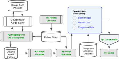
The entire region of interest is partitioned into a “fishnet”, a block of fixed-sized tiles, and for each tile the corresponding satellite image is extracted. The system’s foundation revolves around this fishnet. The approach of partitioning a larger geographical region into smaller, uniformly sized areas offers distinct advantages in granularity, facilitating analysis at the desired level of detail as one can combine tiles for a broader perspective and analyze individual tiles for finer resolution. By selecting a subset of tiles, focus can be directed toward a specific region of interest, ensuring both concentration and consistency throughout the code as each spatial point is mapped to its corresponding tile. Additionally, this method helps overcome challenges related to data management, particularly with large-scale satellite imagery, by facilitating quicker exportation and loading of data. It also supports comparative analysis by allowing the extraction of features for regions of equal size, enabling comparisons between different areas based on these features. Furthermore, the features extracted from each region, including the images corresponding to the tiles, can be seamlessly integrated into machine learning models.
The fishnet outline is initialized through either the minimum and maximum latitude and longitude or by providing a shapefile, as well as a parameter specifying the size of each tile. The above pseudocode (Algorithm 1) outlines the process of generating a fishnet grid for spatial data analysis.
As a practical way for converting degrees to meters and vice versa, which is necessary to correctly extract images from Google Earth Engine, we employ the Haversine formula. It calculates the great-circle distance between two points on the Earth’s surface, considering their latitude and longitude coordinates. Despite the Earth’s non-perfect spherical shape, the Haversine formula, given by Equation 1, is generally considered a good approximation for such use cases.
| (1) |
where:
-
•
is the distance between the two points,
-
•
is the radius of the Earth,
-
•
are the latitudes of the two points in radians,
-
•
is the difference in latitudes,
-
•
is the difference in longitudes.
Due to the substantial volume of images, the development of an efficient method for extraction is necessary. To give an example, the state of Texas spans approximately 1300 km from north to south and 1250 km from east to west. Utilizing a high-resolution grid with each fishnet tile measuring 400 meters per side, the total is approximately 10 million tiles. It is clear that extracting each image individually would be impractical. However, there is a trade-off with processing time, as many smaller images are faster to process than few bigger ones. To process and analyze such large scale of images, we employ a batching approach. Considering a batch size of 64 km per side, around 400 batch images would be required to comprehensively cover Texas. Extracting 400 high dimension images is much easier than extracting millions of smaller ones; at the same time, pre-processing 400 images is faster than pre-processing a dozen of images representing the whole region.

Figure 2 illustrates the batching process. This methodology allows for efficient data extraction for each fishnet tile while optimizing for computational resources.
The ImageExporter module is responsible for using the Earth Engine Python API and builds upon the Python GeeMap package to implement the data extraction process. Rather than using the native JavaScript approach to interact with Google Earth Engine Code Editor, we devised a scalable and development-ready data extraction pipeline using Python. This module adeptly converts Python code into Javascript queries, dispatched to the Earth Engine API, facilitating the extraction of images that are subsequently stored in a designated Google Drive folder.
To test our downstream urbanization prediction task, we needed to obtain a single image per year for each fishnet tile spanning from 2016 to 2022. This is generalizable to extracting images between any year_start and year_end. Although it’s feasible to retrieve any image from a single time stamp within the year in question (say at the beginning or the end of the year), we chose to employ aggregation techniques to create a composite image.
This process entails extracting multiple images for the same year, resulting in an image collection corresponding to multiple timestamps of one fishnet tile, and then applying pixel-level aggregation operations. Some of the available aggregation operations are average, minimum, maximum, median, etc. The advantage of retrieving an aggregated image over a single image lies in noise reduction, with noise stemming from various factors such as cloud cover or sensor noise. The Google Earth Engine offering has built-in functions for aggregating image collections into a single image, however, we opted to incorporate image aggregation in our ImageCorrector module to avoid needing to re-download images in case a different aggregation technique becomes necessary.
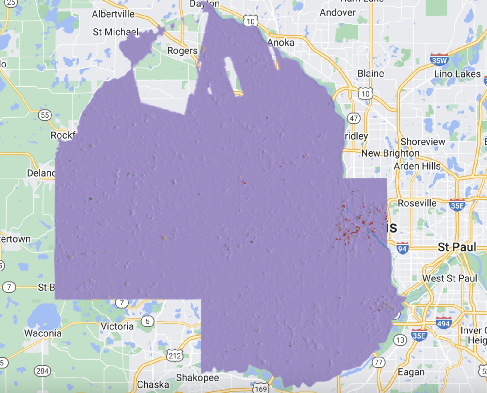
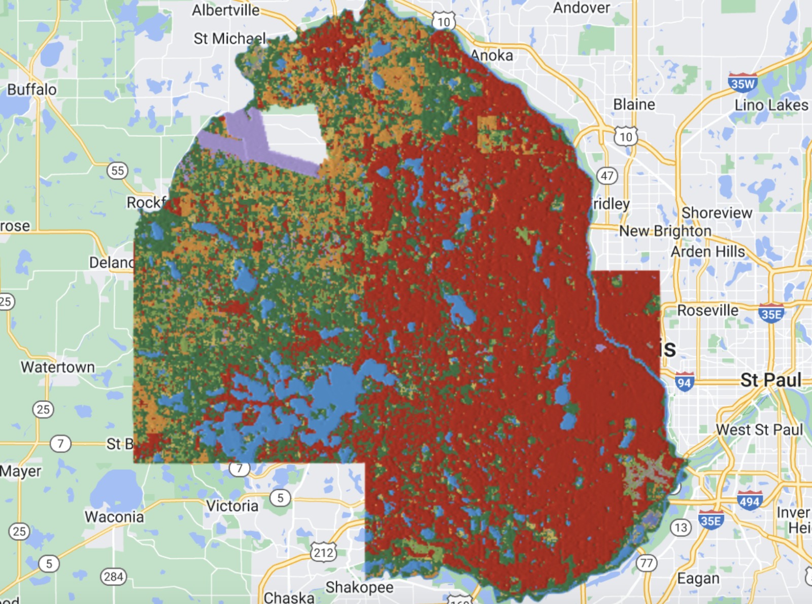
To address the challenges of seasonal variations, especially in cold regions where snow significantly affects land cover visibility in satellite imagery (Figure 3), we only extracted and then aggregated images from summer months (June 1st to October 1st). This period is chosen because it offers a clearer view of labels in their most representative state, free from snow coverage that can mask the underlying land features.
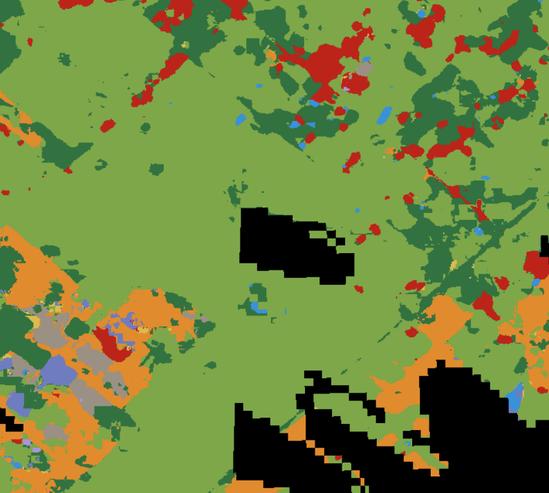
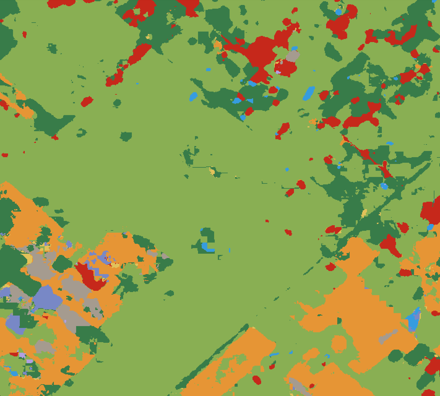
While this strategy is successful in avoiding snow coverage and correctly capturing vegetation, it also encounters obstacles, such as cloud cover, which has particularly impacted data completeness in 2016 and 2017. To rectify instances of missing data caused by clouds, the ImageCorrector module includes imputation techniques, drawing missing pixels from images aggregated over a longer time period which are free from missingness. An example of this can be seen in Figure 4.

Finally, the ImageProcessor class computes various aggregate metrics, such as the percentage of pixels with a certain value within each cell. These aggregate metrics are stored in tabular form, indexed by the unique fishnet tile identifier.
IV Application Case Study and Results
In this work we proposed a standardized extraction, pre-processing and representation pipeline for satellite images. Rather than performing this process in a one-off basis, our approach decreases the time and effort needed to obtain quality representations, freeing resources for data analysis or machine learning and obtaining quality results in a fraction of the time. To showcase our pipeline, we demonstrate how it can be used to build a competitive model for urbanization prediction.
Predicting the future state of a fishnet tile is complex because it involves understanding both temporal and spatial relationships in the input features as well as the dynamics of these relationships in areas with different growth profiles. The goal of this case study is to prove that with the data extraction and pre-processing pipeline previously described, even a complex task such as video prediction for urbanization forecasting is relatively simple to implement and achieves good results.
The model input is a sequence of satellite images from different years processed through our pipeline that can be conceptually regarded as a video, where each image serves as an individual frame (Figure 5). Through a sliding window mechanism, we train the model to predict the region’s future state based on the previous N (here, N = 4) frames.
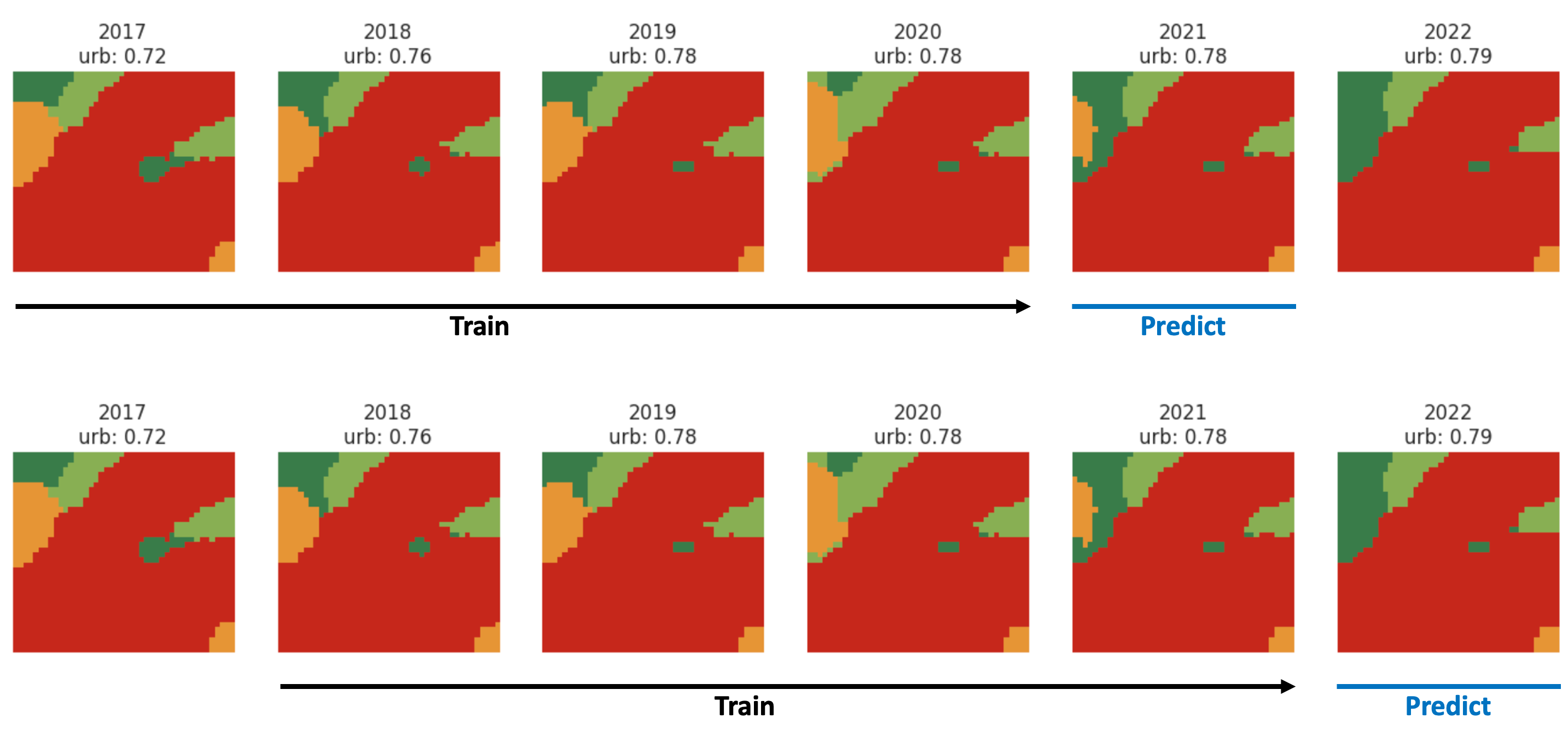
Figure 6 shows a diagram of our model architecture. First, the time series of images is fed into an XGBoost Classifier, trained to solve a binary classification problem, and the area/region is classified as actively urbanizing or passively stabilized. Actively urbanizing regions are fed into a ConvLSTM video prediction model that takes as input the sequence of images. Static regions are fed to an XGBoost Regressor model trained on tabular urbanization information extracted using the ImageProcessor method. More specifically, from each tile, the ImageProcessor method extracts the average number of urbanized pixels for different years to build a tabular dataset, as can be seen in 5. Both models predict the next state of the region in the sequence, represented by the proportion of urbanized pixels in the area. Finally, the predictions from both branches of the pipeline are combined to produce a final urbanization prediction for the tile. We call XBCLM the overall model architecture.

The need for the initial XGBoost classifier stems from the lack of or minimal change over time in most fishnet tiles, a characteristic associated with all LULC satellite products. This poses a significant issue since deep learning models can get trapped in local minima, forecasting little to no change in the majority of fishnet tiles. The initial classifier prevents this issue, making XBCLM a powerful architecture. XGBoost was chosen for its known performance in terms of speed and accuracy; due to the case-study nature of this task, we did not assess different model choices.
As a comparison to XBCLM, we also trained the ConvLSTM with a customized loss function which puts a higher weight on urbanizing pixels to discourage the model from predicting no change. Instead of the typical MSE loss, as shown in equation 2,
| (2) |
we implemented the custom Weighted MSE (WMSE), shown in equation 3.
| (3) |
where:
-
•
() is a multiplier to model increased focus on urbanizing pixels (in our case W=100),
-
•
() represents whether element is an urbanizing pixel or not
While this slightly improved model performance, it did not give significantly better results, so XBCLM is the chosen approach.
Our study presents results derived from training on two distinct data modalities. XBCLM trained on satellite images is benchmarked against an XGBoost regressor which takes as input tabular features extracted from the tiles by the ImageProcessor method.
Both models’ output is a single value representing the tile’s proportion of urbanized pixels in the future. More formally, the XGBoost regressor takes as input a dataframe that lives in , where denotes the total number of tiles and represents the number of years used as features. The output is a vector in . XBCLM takes as input sequences of images, and also returns a vector in . We trained three ensemble and three XGBoost models, each predicting the urbanization proportion of a tile across different future time horizons: 1 year, 2 years, and 3 years in advance. More specifically, we use images from 2016 to 2019 to predict the state in 2020 (1 year in advance prediction), 2021 (2 years in advance) and 2022 (3 years in advance). This approach not only underscores the robustness of our proposed pre-processing pipeline in signal extraction, but also underscores its adaptability across different modalities.
To prevent data leakage between training, validation, and testing phases, we selected entirely distinct regions for each set. Specifically, we utilized the state of Texas for training, Georgia for validation, and Alabama for testing. While we acknowledge that testing the models on additional regions would contribute to more robust results, the primary focus of this paper is on the data pre-processing pipeline rather than the machine learning model itself. Therefore, we limited our testing to these regions.
The results of the XGBoost regressor model are compared to those of the XGCLM model framework in Table 7.
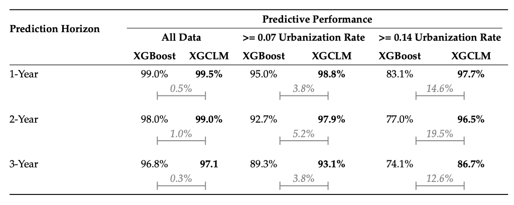
The suggested pre-processing pipeline enables the extraction of data from various modalities, facilitating the training of both XGCLM and XGBoost Regressor models. As seen in the table, the XGCLM model outperforms the XGBoost Regressor at all time horizons. Interestingly, the higher the urbanization rate, the better the performance of the XGCLM model compared to the XGBoost Regresor. This demonstrates that video prediction is able to capture the dynamics of the data at different rates of urbanization.
It is important to note that tends to be very high even for the XGBoost model, especially in areas that do not urbanize quickly. The reason is that, at the tile level, change happens rarely and slowly.
Depending on the training complexity and performance needed, one can opt to train on either tabular data or images directly. Our work accommodates both modeling approaches, and the impressive performance of both XGBoost and XGCLM models highlights the quality and stability of our pre-processing pipeline.
V Interesting Research Avenues
Our current pipeline is primarily structured to handle LULC satellite images. However, a potential enhancement to this study would be to expand the pipeline’s capabilities to seamlessly process various other types of satellite imagery, each encoding different information. In this case, the output would contain multiple customizable information layers, providing a more comprehensive and tailored analysis.
For instance, in our urbanization prediction case study, incorporating nighttime lights imagery could prove valuable in identifying urban areas and monitoring their growth patterns. Other relevant data sources could include surface temperature measurements, air quality indices, cloud coverage maps, or wildlife distribution data. By integrating these diverse information layers, our analysis could gain deeper insights and produce more accurate and holistic predictions.
Another promising research avenue would be to test this approach across a diverse range of Dynamic World labels and study topics such as deforestation, annual snow patterns in the Alps, and agricultural land use dynamics. By applying our methodology to these varied contexts, we could broaden its applicability and evaluate its efficacy in addressing diverse environmental and land-use challenges. Such case studies would not only validate the model’s versatility but also provide valuable insights into different geographical and ecological phenomena, contributing to a more comprehensive understanding of the Earth’s dynamic systems.
VI Conclusion
Our study introduces a standardized pipeline tailored for the extraction, pre-processing, and representation of LULC data sourced from the Dynamic World dataset. As proof of the efficacy of our pre-processing pipeline, we present a predictive model trained on images pre-processed through our pipeline. Results on urbanization patterns show that this model is capable of forecasting future states of LULC labels.
One of the principal strengths of our pipeline lies in its accessibility and user-friendliness. By automating the extraction and pre-processing of satellite images, our approach requires minimal user input, streamlining the generation of analysis-ready datasets. It also ensures standardization and simplifies benchmarking for downstream models, addressing the limitations of heterogeneous custom pipelines. Moreover, our pipeline facilitates the representation of satellite imagery in tabular formats, enhancing versatility for subsequent analytical tasks. The seamless integration between image and tabular data enables researchers to approach analysis and prediction tasks through diverse modalities, catering to the specific requirements of each task.
Addressing the inherent challenge of predicting LULC changes, we devised a two-stage modeling approach. First, our model distinguishes between regions with high urbanization and those with low urbanization using a classification model. Depending on its classification prediction, the information is fed into one of the two potential predictive models, each responsible for estimating the magnitude of urbanization change. Our model is able to predict future urbanization with high accuracy, outperforming the baseline significantly in areas where the rate of urbanization is high.
By reducing the overhead associated with data pre-processing, our model unlocks the rich information contained in the Dynamic World dataset and facilitates the exploration of environmental changes, population movements, and weather phenomena. We advocate for the broader adoption of our extraction pipeline to foster advancements in remote sensing research and its application across various domains.
Acknowledgments
We extend our gratitude to the MIT Sloan School of Management for their support through the Master of Business Analytics (MBAn) capstone project, which provided essential resources for this study. Additionally, we would like to acknowledge JP Morgan for their contribution in supplying resources that facilitated our research.
Data Availability
For this study, we exclusively utilized the Dynamic World dataset. No new data were created during our research. The Dynamic World dataset, which supports our findings, is publicly available and can be accessed through Google’s Earth Engine platform. This dataset provides global land cover classification at high temporal resolution, allowing for detailed analysis of land use and land cover changes over time. Further information on accessing and using the Dynamic World dataset can be found at the official Google Earth Engine data catalog.
Disclaimer
This paper was prepared for informational purposes by the Artificial Intelligence Research group of J.P. Morgan Chase & Co. and its affiliates (“JP Morgan”), and is not a product of the Research Department of JP Morgan. JP Morgan makes no representation and warranty whatsoever and disclaims all liability, for the completeness, accuracy or reliability of the information contained herein.
Abbreviations
The following abbreviations are used in this manuscript:
| DW | Dynamic World |
|---|---|
| convLSTM | Convolutional Long Short-Term Memory |
| XGBoost | eXtreme Gradient Boosting |
| LULC | Land Use and Land Cover |
| UEP | Urban Expansion Prediction |
| XGCLM | XGBoost-ConvLSTM Model |
References
- [1] E. L. Andrews, “Detecting Modern-Day Slavery From the Sky,” Apr. 2024, [Online; accessed 9. Apr. 2024]. [Online]. Available: https://hai.stanford.edu/news/detecting-modern-day-slavery-sky
- [2] F. Karimi and S. Sultana, “Urban Expansion Prediction and Land Use/Land Cover Change Modeling for Sustainable Urban Development,” Sustainability, vol. 16, no. 6, p. 2285, Mar. 2024.
- [3] W. Shuangao, R. Padmanaban, A. A. Mbanze, J. M. N. Silva, M. Shamsudeen, P. Cabral, and F. S. Campos, “Using Satellite Image Fusion to Evaluate the Impact of Land Use Changes on Ecosystem Services and Their Economic Values,” Remote Sens., vol. 13, no. 5, p. 851, Feb. 2021.
- [4] C. F. Brown, S. P. Brumby, B. Guzder-Williams, T. Birch, S. B. Hyde, J. Mazzariello, W. Czerwinski, V. J. Pasquarella, R. Haertel, S. Ilyushchenko, K. Schwehr, M. Weisse, F. Stolle, C. Hanson, O. Guinan, R. Moore, and A. M. Tait, “Dynamic World, Near real-time global 10 m land use land cover mapping,” Sci. Data, vol. 9, no. 251, pp. 1–17, Jun. 2022.
- [5] E. Rolf, K. Klemmer, C. Robinson, and H. Kerner, “Mission critical – satellite data is a distinct modality in machine learning,” 2024.
- [6] J. Chen, J. Chen, A. Liao, X. Cao, L. Chen, X. Chen, C. He, G. Han, S. Peng, M. Lu, W. Zhang, X. Tong, and J. Mills, “Global land cover mapping at 30 m resolution: A pok-based operational approach,” ISPRS Journal of Photogrammetry and Remote Sensing, vol. 103, 10 2014.
- [7] N. Gorelick, M. Hancher, M. Dixon, S. Ilyushchenko, D. Thau, and R. Moore, “Google earth engine: Planetary-scale geospatial analysis for everyone,” Remote Sensing of Environment, 2017. [Online]. Available: https://doi.org/10.1016/j.rse.2017.06.031
- [8] “National Land Cover Database U.S. Geological Survey,” Apr. 2024, [Online; accessed 6. Apr. 2024]. [Online]. Available: https://www.usgs.gov/centers/eros/science/national-land-cover-database
- [9] A. Azabdaftari and F. Sunar, “District-based urban expansion monitoring using multitemporal satellite data: application in two mega cities,” Environmental Monitoring and Assessment, vol. 194, 05 2022.
- [10] A. F. Alqurashi, L. Kumar, and P. Sinha, “Urban land cover change modelling using time-series satellite images: A case study of urban growth in five cities of saudi arabia,” Remote Sensing, vol. 8, no. 10, 2016. [Online]. Available: https://www.mdpi.com/2072-4292/8/10/838
- [11] B. Ahmed and R. Ahmed, “Modeling urban land cover growth dynamics using multi‑temporal satellite images: A case study of dhaka, bangladesh,” ISPRS International Journal of Geo-Information, vol. 1, no. 1, pp. 3–31, 2012. [Online]. Available: https://www.mdpi.com/2220-9964/1/1/3
- [12] A. Manu, Y. Twumasi, K. Lu, and T. Coleman, “Predicting urban growth of a developing country city using a statistical modeling approach,” International Journal of Geomatics and Geosciences, vol. 5, pp. 603–613, 05 2015.
- [13] A. Jaad and K. Abdelghany, “The story of five mena cities: Urban growth prediction modeling using remote sensing and video analytics,” Cities, vol. 118, p. 103393, 11 2021.
- [14] G. Warth, A. Braun, O. Assmann, K. Fleckenstein, and V. Hochschild, “Prediction of socio‐economic indicators for urban planning using vhr satellite imagery and spatial analysis,” Remote Sensing, vol. 12, 05 2020.
- [15] O. R. El-Kawy, H. Ismail, H. Yehia, and M. A.Allam, “Temporal detection and prediction of agricultural land consumption by urbanization using remote sensing,” The Egyptian Journal of Remote Sensing and Space Science, vol. 22, 05 2019.
- [16] H. Taubenböck, T. Esch, A. Felbier, M. Wiesner, A. Roth, and S. Dech, “Monitoring urbanization in mega cities from space,” Remote Sensing of Environment, vol. 117, pp. 162–176, 02 2012.
- [17] V. Sivakumar, “Urban mapping and growth prediction using remote sensing and gis techniques, pune, india,” The International Archives of the Photogrammetry, Remote Sensing and Spatial Information Sciences, vol. XL-8, pp. 967–970, 2014. [Online]. Available: https://isprs-archives.copernicus.org/articles/XL-8/967/2014/
- [18] M. Ahadnejad Reveshty, “The assessment and predicting of land use changes to urban area using multi-temporal satellite imagery and gis: A case study on zanjan, iran (1984-2011),” J. Geographic Information System, vol. 3, pp. 298–305, 01 2011.
- [19] D. Aldogom, N. Aburaed, M. Al-Saad, S. Al Mansoori, M. Shamsi, and A. Maazmi, “Multi temporal satellite images for growth detection and urban sprawl analysis; dubai city, uae,” Remote Sensing Technologies and Applications in Urban Environments, p. 16, 10 2019.
- [20] B. Frimpong, “Tracking urban expansion using random forests for the classification of landsat imagery (1986–2015) and predicting urban/built-up areas for 2025: A study of the kumasi metropolis, ghana,” Land, vol. 10, 01 2021.
- [21] S. Alkheder and J. Shan, “Urban growth simulation using remote sensing imagery and neural networks,” International Society for Photogrammetry and Remote Sensing, 05 2012.
- [22] W. Boulila, H. Ghandorh, M. Ahmed Khan, F. Ahmed, and J. Ahmad, “A novel cnn-lstm-based approach to predict urban expansion,” 03 2021.
- [23] C. A. F. de Sousa, J. A. R. da Silveira, C. A. G. Santos, and R. M. da Silva, “A methodological proposal to analyze urban sprawl, negative environmental impacts, and land degradation in the case of joão pessoa city (brazil) between 1991 and 2018,” Environmental Monitoring and Assessment, vol. 195, no. 6, p. 738, 2023.
- [24] E. Şahin and M. C. İban, “Investigation of land use change and urban sprawl around mersin city hospital,” in INTERNATIONAL GRADUATE RESEARCH SYMPOSIUM IGRS’22 E-ABSTRACT BOOK, 2022, p. 382.
- [25] B. Praveen, S. Parveen, and V. Akram, “Urban change detection analysis using big data and machine learning: A review,” Advancements in Urban Environmental Studies: Application of Geospatial Technology and Artificial Intelligence in Urban Studies, pp. 125–133, 2023.
- [26] K. M. Gilbert and Y. Shi, “Urban growth monitoring and prediction using remote sensing urban monitoring indices approach and integrating ca-markov model: A case study of lagos city, nigeria,” Sustainability, vol. 16, p. 30, 12 2023.
- [27] H. Liu and Q. Zhou, “Developing urban growth predictions from spatial indicators based on multi-temporal images,” Computers, Environment and Urban Systems, vol. 29, pp. 580–594, 09 2005.
- [28] V. Anand and B. Oinam, “Future land use land cover prediction with special emphasis on urbanization and wetlands,” Remote Sensing Letters, vol. 11, pp. 225–234, 03 2020.
- [29] H. Bagan and Y. Yamagata, “Analysis of urban growth and estimating population density using satellite images of nighttime lights and land-use and population data,” GIScience & Remote Sensing, vol. 52, no. 6, pp. 765–780, 2015. [Online]. Available: https://doi.org/10.1080/15481603.2015.1072400
- [30] R. C. Daudt, B. Le Saux, A. Boulch, and Y. Gousseau, “Urban change detection for multispectral earth observation using convolutional neural networks,” in IGARSS 2018-2018 IEEE International Geoscience and Remote Sensing Symposium. Ieee, 2018, pp. 2115–2118.
- [31] Q. Shi, M. Liu, S. Li, X. Liu, F. Wang, and L. Zhang, “A deeply supervised attention metric-based network and an open aerial image dataset for remote sensing change detection,” IEEE transactions on geoscience and remote sensing, vol. 60, pp. 1–16, 2021.
- [32] S. Hafner, Y. Ban, and A. Nascetti, “Urban change detection using a dual-task siamese network and semi-supervised learning,” in IGARSS 2022-2022 IEEE International Geoscience and Remote Sensing Symposium. IEEE, 2022, pp. 1071–1074.
- [33] X. SHI, Z. Chen, H. Wang, D.-Y. Yeung, W.-k. Wong, and W.-c. WOO, “Convolutional lstm network: A machine learning approach for precipitation nowcasting,” in Advances in Neural Information Processing Systems, C. Cortes, N. Lawrence, D. Lee, M. Sugiyama, and R. Garnett, Eds., vol. 28. Curran Associates, Inc., 2015.