Adaptive Active Inference Agents for Heterogeneous and Lifelong Federated Learning

Abstract

Handling heterogeneity and unpredictability are two core problems in pervasive computing. The challenge is to seamlessly integrate devices with varying computational resources in a dynamic environment to form a cohesive system that can fulfill the needs of all participants. Existing work on systems that adapt to changing requirements typically focuses on optimizing individual variables or low-level Service Level Objectives (SLOs), such as constraining the usage of specific resources. While low-level control mechanisms permit fine-grained control over a system, they introduce considerable complexity, particularly in dynamic environments. To this end, we propose drawing from Active Inference (AIF), a neuroscientific framework for designing adaptive agents. Specifically, we introduce a conceptual agent for heterogeneous pervasive systems that permits setting global systems constraints as high-level SLOs. Instead of manually setting low-level SLOs, the system finds an equilibrium that can adapt to environmental changes. We demonstrate the viability of AIF agents with an extensive experiment design, using heterogeneous and lifelong federated learning as an application scenario. We conduct our experiments on a physical testbed of devices with different resource types and vendor specifications. The results provide convincing evidence that an AIF agent can adapt a system to environmental changes. In particular, the AIF agent can balance competing SLOs in resource heterogeneous environments to ensure up to 98% fulfillment rate.

I introduction

The Distributed Computing Continuum is an emerging paradigm for systems that can seamlessly integrate multiple layers of computing infrastructure [1]. Computing continuum systems promise to enable infrastructure-critical pervasive applications with stringent requirements, such as Mobile Augmented Reality (MAR) for cognitive applications [2] and Remote Sensing for Disaster Management [3]. There are three recurrent characteristics among pervasive applications deployed on a continuum. First is their reliance on AI-based methods for tasks that classical control structures cannot solve efficiently or with sufficient precision [4]. For example, MAR applications must process streams of high-dimensional data that a service could ideally process at the source to fulfill a sub-10 millisecond latency Service Level Objective (SLO). The caveat is that resources in proximity are constrained. Typical solutions involve task partitioning and lightweight data reduction methods that minimize the penalty for offloading to remote resources [5]. The second is heterogeneity, i.e., resource-asymmetry, vendor specifications, and usage patterns. Although pervasive applications follow an overall common objective, a system must consider the individual properties and objectives of participants. The third is the continuously drifting problem domain intrinsic to the dynamic environments of pervasive applications, such that the source distribution drifts over time and data volume is non-static. Conclusively, a necessary precondition is a system that can adapt to non-identically and independently distributed (non-IID) data. Moreover, the system must facilitate collaboration between heterogeneous devices to fulfill their SLOs by distributing workload fairly and considering the individual properties of participants.

The focus is on lifelong heterogeneous federated learning (FL) as we find it best encapsulates the primary challenges of pervasive applications that share the described characteristics. In general, FL participants collaborate for a common objective, i.e., to maximize the prediction performance. Yet, each participant has a private local validation set to determine whether their criteria are locally met. Time constraints that ensure smooth operations and resource asymmetry further instigate friction when attempting to satisfy local objectives. Hence, despite a common objective, to fulfill the SLOs of each participant individually, a delicate balance is necessary. Lastly, the dynamic environment gradually drifts the distribution and varies the data volume.

This work aims to demonstrate the viability of Active Inference (AIF) in designing adaptive agents that can gracefully handle the challenging requirements of pervasive applications. While Active Inference is a neuroscientific framework, recent work has shown promising results by conceiving methods from the underlying ideas for workload scheduling in distributed systems. In particular, we find that the objectives of Active Inference and pervasive computing intrinsically intertwine. Context awareness is crucial for pervasive applications as these systems operate in dynamic environments and must adapt to changes in their surroundings. Precisely context awareness is a defining characteristic of AIF agents. However, the current application of AIF for systems is more conceptual and only partially implements the core components of the AIF framework [6, 7]. Other work on systems that adapt to changing requirements typically focuses on optimizing individual variables, such as learning rate or setting low-level SLOs as constraints on specific resources [8, 9]. Despite providing more fine-grained control, it is unreasonable to expect application developers to understand the implications of each low-level constraint to the overall system, particularly in dynamic environments where resources are scarce and availability is less predictable. In contrast, our AIF agent permits setting high-level SLO targets to find an equilibrium without attempting to enforce constraints from possibly conflicting low-level SLOs.

We design experiments that accurately reflect the relevant real-world conditions by implementing a physical testbed consisting of heterogeneous devices with varying resource types and computational capabilities. Additionally, we leverage a controlled process for data generation to evaluate the adaptability to a dynamic environment precisely. We extensively evaluate our agents with a strong emphasis on reproducibility. The results underpin the claim that an AIF agent can successfully balance competing SLOs among clients despite considerable resource asymmetry and adapt to the dynamic environment. Still, we transparently discuss current limitations by accentuating the parts of our result that best show our agent’s weaknesses. The intention is to foster research interest in AIF from a systems perspective, as we sincerely believe that it poses an exceptionally promising research direction for pervasive applications and the compute continuum. Naturally, we open-source our repository as an addition to the community to reproduce, scrutinize, and extend our approach .

We summarize our contributions as:

• An adaptive mechanism for heterogeneous lifelong FL based on AIF which allows handling non-IID data distributions and heterogeneous device characteristics inherent in pervasive computing environments.

• A conceptual AIF agent that balances multiple SLOs during model training. When SLOs compete, agents can autonomously infer optimal training configurations without manual intervention.

• The empirical evaluation of AIF agents for pervasive FL tasks; experiments were designed to reflect real-world conditions, such as data and resource heterogeneity

II Background

II-A Lifelong Heterogeneous Federated Learning

In Federated Learning, participants train a global model to maximize prediction performance without disclosing private data. Participants optimize and validate the model parameters with their local dataset in a training round before aggregating their weights globally.

II-A1 Heterogeneous Federated Learning

We refer to Federated Learning as heterogeneous when data is non-IID and hardware specifications vary among participants. Moreover, hardware heterogeneity typically implies that resources are constrained, i.e., to not discriminate against computationally less powerful devices closer to the source.

II-A2 Lifelong Federated Learning

FL is lifelong when training continuously adapts to concept drifts  [10]. Introducing concept drifts is an intrinsic property of the dynamic deployment environment of pervasive applications. Yet, there is limited research interest in lifelong learning for FL [11].

II-A3 Service Level Objectives for Federated Learning

SLOs are definable constraints on a system that operators may use as contracts with application developers [12, 13]. Low-level SLOs quantify directly observable measures, such as CPU or memory usage. High-level SLOs abstract low-level SLOs to reduce the difficulty of diagnosing and configuring complex and wide-spanning systems, i.e., compute continuums with measures such as throughput or monetary costs.

For our purposes, high-level SLOs provide an intuitive interface to set targets for an AIF agent and quantitative measures to determine its adaptability to a dynamic environment. In particular, maintaining prediction performance and minimizing round duration are two primary objectives for lifelong heterogeneous federated learning. An SLO on prediction performance ensures consistent solution quality. In contrast, an SLO on timeliness is crucial as resources are constrained, and a considerably slower client can delay global weight updates.

II-B Active Inference

Active inference is a neuroscientific framework based on the free energy principle (FEP) [14]. AIF agents adjust their model according to new observations and enact environmental changes to suit their preferences. The objective is to minimize the difference between the agent’s internal representation and real-world models, i.e., to adapt to its environment. In principle, the underlying framework of AIF generally applies to adaptive systems [15]. Therefore, it is reasonable to assume that AIF is a promising direction for computing continuums that must adapt to a dynamic environment [6].

AIF agents continuously evaluate the expected free energy (EFE) for different policies and assess their impact on underlying models. In a system’s context, an agent who understands the world model will minimize EFE by selecting policies likely to fulfill SLOs.

We can describe the EFE with two distinct components [16]:

$$\text{EFE}=-\overbrace{\mathbb{E}_{Q(o|\pi)}[\ln P(o|C)]}^{\text{Pragmatic Value}}-\underbrace{\mathbb{E}_{Q(o,s|\pi)}D_{\mathrm{KL}}\left[Q(s|o)\,\|\,Q(s)\right]}_{\text{Information Gain}}$$ (1)

The information gain (IG) estimates how much the model can improve by choosing a particular policy. Conversely, the pragmatic value estimates how close a possible outcome will be to the agent’s preferred state.

III Problem Statement

We consider a lifelong heterogeneous FL system consisting of an orchestrator with $N$ participants. Figure 1 illustrates an example.

Figure 1: Heterogeneous FL with data streams and AIF agents

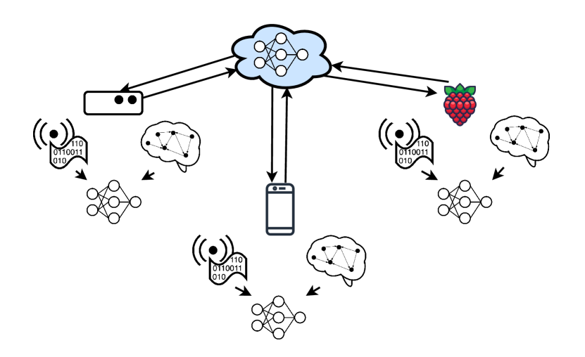
Client hardware is heterogeneous in vendor specification, available resource types, and overall computational capacity. For example, some devices may have onboard accelerators, such as GPUs, and others may only work with energy-efficient CPUs. The data source is non-IID with temporal correlations, i.e., the training must adapt to non-stationary data. SLOs are globally configurable, and clients check after each training round whether the SLOs are fulfilled locally. The SLOs aim to ensure smooth operations, i.e., timely training and consistently adequate model performance. We introduce a mechanism to control and manage SLO fulfillment by defining FL training configurations, which specify training parameters that directly affect the system’s ability to fulfill SLOs. Configurations function as levers that an agent can change to fulfill the user-set high-level SLOs. The objective is for the FL system to maximize the overall SLO fulfillment across all timestamps. The challenge is to ensure the highest possible SLO fulfillment, given heterogeneous participants and data within a dynamic environment.

The following describes how we can draw from AIF to design agents that can result in a self-adapting SLO-aware system behavior. In short, the agent learns the world model and becomes sensitive to changes, such that it can maintain service quality by reacting to environmental changes.

IV Proposed Method

This section presents the design of the AIF agents that optimize a heterogeneous and lifelong federated system to fulfill SLOs. Figure 2 illustrates how system entities

Figure 2: Sequence diagram for one FL round of the proposed method

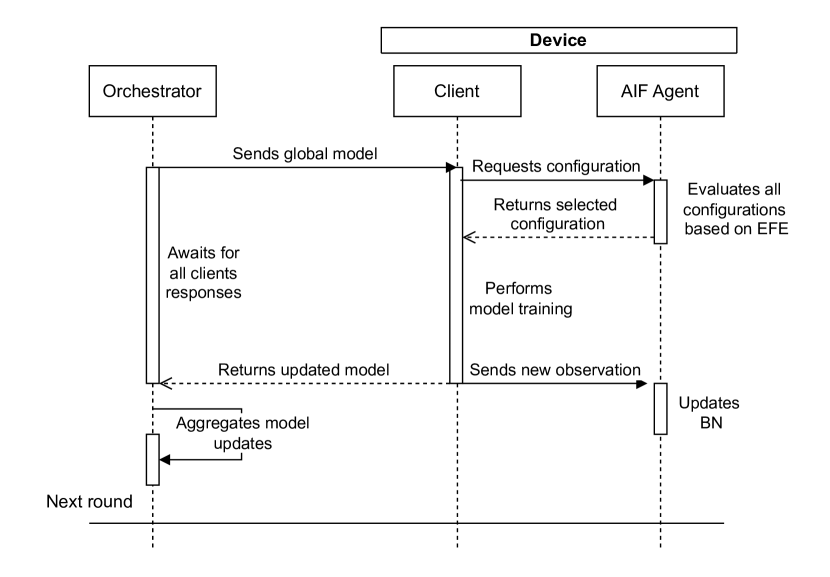
interact. Algorithm 1 summarizes the overall procedure for client-side training.

Procedure train($global\_model$, $is\_lifelong$)

       $train\_set$ $\leftarrow$ fetch_next_train_set()

       $config$, $expected\_ig$ $\leftarrow$ infer_best_config()

      

      With $config$:

       $updated\_model$, $metrics$ $\leftarrow$ train_model($global\_model$, $train\_set$, $config$)

      

      $slos\_fulfilled$ $\leftarrow$ check_slo_fulfillment()

       If $is\_lifelong$:

       $new\_obs$ $\leftarrow$ $slos\_fulfilled$ $\cup$ $config$ $\cup$ $metrics$

      

      update_bn($new\_obs$, $expected\_ig$)

       return $updated\_model$, $metrics$

Procedure infer_best_config()

       $configs\leftarrow\{\}$

       foreach $c$ in $possible\_configs$ do

             $EFE_{c}$, $ig_{c}$ $\leftarrow$ calculate_efe($c$)

             $configs\leftarrow configs\cup(EFE_{c},ig_{c})$

      return $possible\_configs_{\arg\min(\text{configs.EFE})}$

Procedure update_bn($new\_obs$, $expected\_ig$)

       $obs\_surprise$ $\leftarrow$ calculate_surprise($BN$, $new\_obs$)

       if $obs\_surprise>expected\_ig$ then

             $BN\leftarrow$ do_structure_learning()

             $BN\leftarrow$ do_parameter_estimation($BN$)

      else

             $BN\leftarrow$ do_parameter_update($BN$, $new\_obs$)

      

Algorithm 1 On Client Training Procedure

The following elaborates on notable details about the process for an agent to find and choose optimal FL training configurations in a dynamic environment.

IV-A Learning a Simple Causal World Model

The generative model is at the core of an AIF agent, i.e., as an agent interacts with its environment, it updates its internal world representation in a perception-action cycle. We choose Bayesian Networks (BNs) as they provide interpretable graphical representations of learned causal structures. This work considers discrete BNs with uniform priors. Each agent’s initial Bayesian network structure is unknown, as there are no assumptions on prior knowledge of the environmental dynamic. The agents require only starting knowledge of the BN variables and their respective cardinalities. We define the BN $\mathcal{B}$ of an agent as:

$$\mathcal{B}=(\mathcal{G},\mathcal{P})$$

where $\mathcal{G}=(V,E)$ is a directed acyclic graph (DAG), and $\mathcal{P}$ is the set of conditional probability distributions:

$$\mathcal{P}=\{P(X_{i}|\text{Pa}(X_{i}))\}_{i=1}^{n}$$

$\text{Pa}(X_{i})$ represents the parents of $X_{i}$ in $\mathcal{G}$, for which the joint distribution of the variables is factorized as:

$$P(X_{1},X_{2},\dots,X_{n})=\prod_{i=1}^{n}P(X_{i}|\text{Pa}(X_{i}))$$

The BN vertices are divided into three categories:

1. Configuration vertices: Represent the (hyper)parameters of the system that are available for the agent to set.

2. SLO vertices: Binary vertices that encode SLO being fulfilled or not and allow for finding dependencies between SLOs (and their fulfillment) and other vertices of the BN.

3. System vertices: Additional vertices provide a more comprehensive overview of the system dynamic, such as resource usage, and their connection to SLOs.

We use Hill Climb Search [17] and Bayesian estimation to perform structural learning and parameter estimation. We use variable estimation to perform exact inference, such that an AIF agent utilizes precise computation to leverage the uncertainty of BNs. As the FL rounds progress, the BN causal structures are progressively discovered. Moreover, the agent experiences further refine the conditional probability distributions.

IV-B EFE and SLO-aware Configuration Selection

Due to SLO and configuration vertices present in the BN, the task is to correctly discover the connections between the vertices to choose the configuration with the highest chance of fulfilling SLOs. The agent calculates the EFE for each configuration available to the system to determine configuration optimality using the formula in Equation 1. Specifically, it calculates the pragmatic value as:

Pragmatic Value $$=\sum_{\text{SLOs}}P(\text{SLOs}\mid\text{configuration})$$ (2)

$$\times\text{preference vector}$$ (3)

and the Information Gain as:

$$\text{Information Gain}=I(\mathcal{A},\mathbf{q})$$ (4)

The preference vector encodes the agent’s goal, i.e., the desired outcome, and is expressed as a logarithm of the normalized preferences. The list of outcomes consists of all combinations of possible SLOs values. Since the agent is to fulfill all set SLOs, the state where all SLOs are fulfilled will have a higher preference. For example, for one binary outcome SLO, one can set the preference vector to [0.001, 0.999], specifying that the second outcome is preferred. Information gain quantifies the expected Bayesian surprise that measures how much observing new data would update the agent’s belief about hidden states. Following the implementation in [18], the calculation uses the likelihood of SLOs fulfillment under configurations (matrix $A$) and the predictive density over hidden states $q$ derived from the Bayesian Network. An observation is a configuration and an associated outcome. The agent uses a particular configuration as evidence to predict the possible observation with a maximum a posteriori (MAP) query to simulate possible future and predict its IG. In summary, the information gain and pragmatic value balance a trade-off between exploring and taking the actions that most likely result in SLOs fulfillment. Once the agent has selected a configuration, the local training round starts. On completion, the agent collects lower-level metrics and checks SLO fulfillment. Lastly, it associates the outcomes with the configuration and adds it to the history dataset as a new observation for further updates. A BN update step can result in a parameter update or structure learning followed by a parameter estimation. Figure 3 illustrates the process of learning the structure of the BN as the FL rounds progress.

Figure 3: BN structure update throughout FL training rounds (blue vertices represent SLOs, green – configuration variables)

We distinguish between two update types to allow the agent to adapt to significant discrepancies between expected and observed outcomes. If the observed IG is higher than expected, the agent discards structure information from the previous iterations and initializes structure re-learning of the BN. Structure re-learning prioritizes the edges that include SLOs as the dependent node, to ensure that the relations that have an immediate impact on agent decisions are considered first. Conversely, if the observed IG is within expectations, the agent only initializes a parameter update on the BN.

To ensure the BN does not learn from early-stage ML model performance data, that do not accurately describe the relationship between performance SLO and configuration, these observations are omitted until the model performance stabilizes. When the global FL model performance gets sufficiently close to the target performance SLO, a lifelong learning flag signals the AIF agent to start learning.

V Evaluation

V-A Experiment Design

The experiment design examines the AIF agent’s behavior and adaptability to heterogeneity and lifelong FL.

V-A1 Test Bed

We implement a physical testbed with constrained devices to replicate a heterogeneous resource environment. Additionally, we use a virtual machine with server-grade hardware for experiments in more controlled environments. Table I summarizes the hardware specifications.

TABLE I: Testbed Hardware Specifications

Device	CPU	Accelerator
Virtual Machine	8x Xeon @ 3.7 GHz	Tes. 2560 CC
Orin NX	8x Cortex @ 2 GHz	Amp. 1024 CC 32 TC
Xavier NX	4x Cortex @ 2 GHz	Vol. 384 CC 48 TC
Raspberry Pi 4	4x Cortex @ 1.8 GHz	N/A
Raspberry Pi 5	6x Cortex @ 2.0 GHz	N/A

V-A2 Implementation Details

We implement the prediction model as a simple Artificial Neural Network (ANN) with PyTorch consisting of two fully connected layers using ReLU activation for non-linearity.

We extend the Flower [19] framework to support FL. We implement the agent BNs with pgmpy [20] and information gain with pymdp [18]. We implement a controllable data generation process using River [21]. A more detailed technical description is out of scope and we refer interested readers to the accompanying repository.

V-A3 Application Scenario

We emulate a dynamic environment by controlling the data generation process to introduce concept and volume drifts. Each client device represents a different participant. The challenge is, for the system to adapt to the drifts or to the varying computational resources of participants. The experiments consider the fulfillment of two high-level SLOs:

1. Time: fulfilled if a local training round does not exceed a set limit (e.g., 2 seconds).

2. Prediction Performance: fulfilled if the primary validation metric (accuracy) exceeds a set value.

We choose time and performance as SLOs as balancing them is non-trivial. For example, focusing exclusively on fulfilling prediction performance may require spending an excessive amount of time and vice versa. The configurable hyperparameters are Batch Size $BS\in\{8,32,64,256,512\}$ and Learning Rate $LR\in\{0.0005,0.001,0.005,0.01\}$, as there is a clear connection to them and the system’s training objective and considered drift types, e.g. learning rate tuning was proposed to battle concept drift [11]. Each client initialized a separate datastream locally, using their identifier as a random seed for the stream to promote variability in the data across clients. However, the rest of the data stream parameters were set to the same values across clients inside one run. This way, the number of features and classes are kept the same, showcasing that all clients are part of the same ML task. Other parameters, such as the number of clusters (groups of data points represented by centroids), the random seed for cluster initialization, and the cluster drift, are kept constant to ensure a proper comparison of the agents’/clients’ behavior and to maintain the reproducibility of the generated data inside one repetition. The data generator $G$ is also parametrized by a drift parameter, $drift$, which controls the presence and speed of data drifts, where $drift=0$ indicates no data drift.

In each federated round, clients train and validate their prediction model using the data samples available in an online learning fashion. At round $t$, each client $n$ possesses two datasets: $\text{Validation}_{t}=\{(x_{b},y_{b})\}_{b=1}^{B_{t}}\sim G_{n}$ and $\text{Train}_{t}=\text{Validation}_{t-1}$, where $x$ is a feature vector, $y$ label assigned to the data sample and $B_{t}$ the size of the data set drawn from the data generator at round $t$.

This way, clients acquire a new batch of data for validation while the previous batch is re-used for training. Previous round training samples are discarded.

V-A4 Baselines

The baselines focus on the best- and worst-case scenarios rather than existing methods to avoid misleading comparisons with the tangentially related problem definitions and methods and concentrate on depicting the dynamics and capabilities of AIF agents. We define two baselines for experiments with data distribution drifts:

1. Random: Represents a complete lack of adaptability and intelligent choice of hyperparameters. This baseline randomly chooses a new configuration for each federated training round.

2. Fixed optimal: Represents the case where parameter tuning was performed and the optimal configuration is set once at the beginning of the training and is never changed. To select this configuration, each of the possible configurations was tested and the one with the highest mean SLOs fulfillment at the end of the observed period (around round 50) was taken as the optimal.

Cumulative SLO fulfillment at round $t$ is calculated as:

$$\text{SLO Fulfillment}_{t}=\frac{\sum_{i=1}^{t}\text{SLO fulfilled}_{i}}{t}$$ (5)

Each experiment was repeated ten times with different random seeds that controlled the random processes, such as the data generator and ANN weights initialization. For the evaluation, the first considered timestep included in SLO fulfillment tracking for a particular client run was the one where the “lifelong” flag becomes true. The reported results are averaged across all participating clients and experiments, if not stated otherwise. The number of local epochs was set to 3 for all experiments with no client subsampling, i.e., all FL clients participated in every round. The SGD optimizer was used by default. It is also worth reminding that agents learn their BNs from scratch in every experiment.

V-B Results

Each experiment describes the results regarding SLO fulfillment, as the evaluation metric expected by the users, and EFE dynamics that explain the learning and adaptation of AIF agents.

V-B1 Data Heterogeneity

Consider a real-life situation where clients experience changes in the amount of collected data, e.g., seasonal demands in shops specializing in certain types of products or bursts of the number of service requests. For this experiment, such quantity drift is modeled by increasing the number of samples drawn from the data generator every 50 epochs, starting with 5,000 samples, then increasing to 10,000 and 15,000. The SLOs were set to 2 seconds for time and 97% for model performance SLO. The number of federated clients was set to 10.

The dynamic of both SLO fulfillments is shown in Figure 4.

Figure 4: Mean cumulative SLOs fulfillment with two quantity drifts (red lines mark the drift start). Semitransparent lines show mean SLO fulfillment at a single federated round.

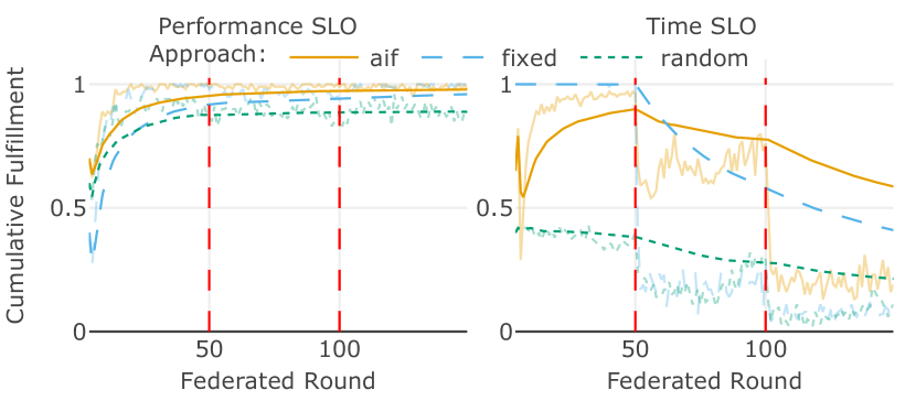
For the fixed “optimal” baseline, the cumulative fulfillment was high for both SLOs until the first quantity drift occurred at the 50th round. After this round, time SLO stopped being consistently fulfilled, which led to a steady decline in time SLO fulfillment. However, looking at the AIF approach, it is evident that despite the time SLO becoming more challenging to fulfill, it still manages to recover after the quantity drift, with the mean time SLO fulfillment per round being consistently larger than 50%. Still, after the second quantity drift happened, the time SLO became even more challenging, which led to a more prominent decline in time SLO fulfillment. To understand the choices made by the AIF agents, we examine mean EFE over all configurations at each epoch (Figure 5).

Figure 5: Mean EFE with two quantity drifts with each line representing one possible training configuration. Lower values represent configurations that the AIF agents favor.

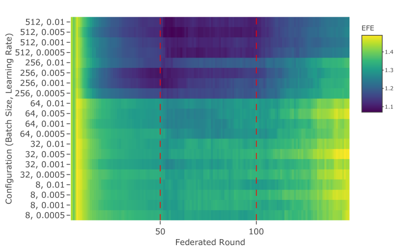
It is visible how the configurations preferred by the AIF agents change after the observed environmental changes. In the beginning, it is shown how agents slowly come to prefer configurations (256, 0.005) and (256, 0.001) (compared to the fixed baseline being (256, 0.01)). However, after the first quantity drift, this preference shifted to a larger batch size of 512. This is an expected behavior as the amount of data doubled, but the time constraint remained the same. Still, after the amount of data increased again, there was no more space to increase the batch size. Therefore, the increase of EFE across all configurations can be observed, signaling that.

As shown in Equation (1), the information gain term accounts for explorative behavior and is compared to the actual observed information gain during each federated round to estimate how “surprised” the agent is. Figure 6 a shows the mean information gain across clients.

Figure 6: a) Mean observed IG over all clients and repetitions, b) Observed and expected information gain for one client at one run

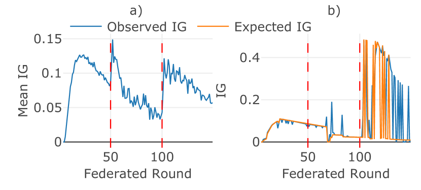
Here, the process of agents adapting to the environment can be seen, with the observed IG decreasing as the BN becomes more confident. However, two prominent spikes occur right after the quantity drifts, illustrating the “surprised” agents detecting the environmental change.

To better illustrate the dynamics of looking for the best configuration after the second quantity drift, the entire history of expected and observed IG of one client can be observed (Figure 6 b). This client initially settled down for a configuration of (512, 0,01), which worked for the agent for 68 epochs due to the observed IG being less or equal to the agent’s expectations. However, at round 68, the agent was surprised because the time SLO was not fulfilled despite using the “time-proven” configuration. Despite being surprised, the agent only retrained the structure of the BN (indicated by the abrupt change in the expected IG). It happened several times more, but the agent preferred exploiting its knowledge. After round 100, the agent again started to be surprised, leading to a change in strategy. The agent went exploring, as visible by the increased expected information gain. These spikes are also associated with the agent choosing previously unexplored (or poorly explored) configurations. For instance, round 104 corresponds to the agent choosing configuration (64, 0.005). This example illustrates how AIF agents treat changes in the observed environment and can independently balance between exploration and exploitation.

As the setup for the experiment consisted of ten clients and ten separate experiments, it is possible to represent configurations preferred by the agents at three critical points (before the first quantity drift, before the second quantity drift, and at the end of the experiment) into distributions over configurations. These distributions are given in Figure 7.

Figure 7: Chosen configurations distributions before and after quantity drifts

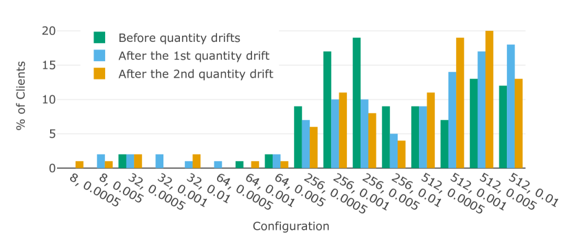
Despite the expected behavior, a minority of agents still settle for clearly non-optimal configurations. Another observation is the shift in the preferred configurations after the first quantity drift towards a bigger batch size. To quantify the observed changes in the distributions, Fisher’s exact test was performed on the distributions with batch sizes 256 and 512 (too low values were filtered out to focus the test on the sensible configurations as the rest represent wrong configurations and are irrelevant for the test). The p-value of this test was reported to be 0.0293, showing the statistical significance in the observed changes between the distribution of the preferred configurations before and after the first quantity drift.

Observed EFE after the second quantity drift shows that the agents’ behavior is dictated by the combination of available configurations and set SLOs. To better estimate the effect SLOs have on the preferred configurations, a set of experiments was conducted that modified the SLOs considered in the experiments. Table II shows the SLOs chosen for each experiment compared to the SLOs considered in the previous experiment.

TABLE II: Comparison of Time and Performance SLOs for Different Experiments

Experiment	Time SLO (s)	Performance SLO (%)
Fullfiable SLOs	2	97
Unfulfillable SLOs	0.1	99.5
Easily Fullfillable SLOs	3600	50
Time Relaxed	3600	97
Performance Relaxed	2	50

Figure 8 shows the mean EFE over five clients used for experiments and ten repetitions.

Figure 8: Mean EFE under different SLOs setups and two quantity drifts

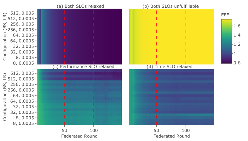
The EFE shows that having not challenging or unrealistic SLOs (Figure 8 a and b, respectively) leads to EFE being consistent across all available configurations, with EFE being high when the target SLOs are unfulfillable and EFE being equally low when the targets are too easy to fulfill. The situation is different when one of the two SLOs is relaxed while the other is somehow challenging to fulfill. Thus, when performance is relaxed, the agents are incentivized to optimize the behavior towards time SLO, leading to agents settling for the largest available batch size (512) regardless of the learning rate. The situation is different regarding time-relaxed SLO – when the performance is targeted, agents tend to explore more configurations as the task is still not that challenging for them, leading to diverse behaviors. Still, the resulting EFE heatmap expresses some preference bias compared to the experiment with two SLOs relaxed. This “uncertain” behavior could be attributed to quantity drifts not impacting the performance goals. A situation where time is relaxed in the presence of concept drift is presented later in this section, illustrating the preferences developed by the agents when model performance (and performance SLO) has a clearer connection with the configurations available.

The following experiment added concept drift to the problem. Concept drift was added to the generator from the start to make the task more complicated, and, as a result, the performance SLO was adjusted to still be challenging yet reachable (85%). One quantity drift was also present (from 10,000 to 15,000 samples), therefore, introducing two sources of data heterogeneity in one experiment. The resulting SLOs fulfillment for 5 FL clients is shown in Figure 9.

Figure 9: Mean SLOs fulfillment under concept drift and 1 quantity drift. Time SLO: 3 seconds, performance SLO: 85%

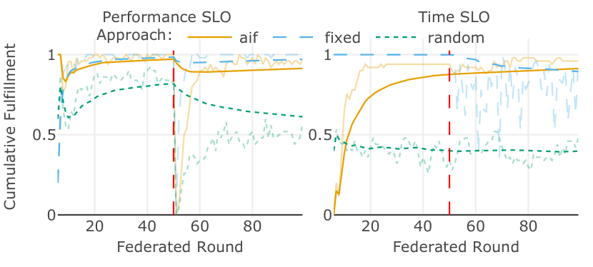
With concept drift, reaching the target performance SLO becomes more challenging. Moreover, when the quantity drift happens – concept drift becomes more prominent in response, as more samples are drawn from the data generator and clusters drift faster. It impacts the model’s performance, as can be seen from the prominent decline of the random baseline, illustrating that fewer configurations can now sustain the performance goals. Despite that, the AIF agent maintains its performance SLO fulfillment and keeps time SLO not impacted by the quantity drift. Here, the agents preferred configurations with larger batch sizes of 256 and 512, with (512 0,0005) having the lowest mean EFE (compared to the fixed baseline being (256, 0.005)).

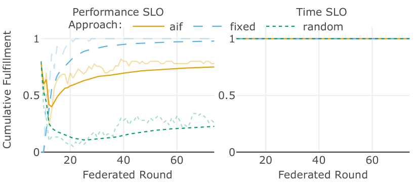
As was previously noted and could be seen from the previous example, concept drift mostly impacts the performance SLO, which is a more nuanced target compared to the time SLO, which is more straightforward to optimize. The experiment containing only more severe concept drift was conducted to better inspect the behavior of AIF agents when facing performance-oriented SLO. Here, the performance SLO was set to 78.5% (due to a more prominent concept drift) and the time SLO was relaxed (3600 s). The performance SLO fulfillment is shown in Figure 10 and the resulting mean EFE is shown in Figure 11.

Figure 10: Mean SLOs fulfillment under concept drift and relaxed time SLO. Time SLO: 2 seconds, performance SLO: 78.5%

Figure 11: Mean EFE under a concept drift with relaxed time SLO

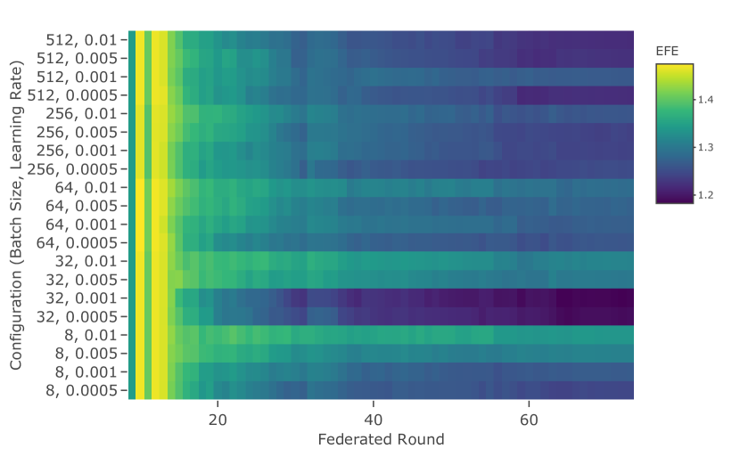
The optimal configuration for the baseline was set to (64, 0.001), and it is shown from the mean EFE that agents also preferred a lower batch size of 32 and lower learning rates of 0.0005 and 0.001.

V-B2 Device Heterogeneity

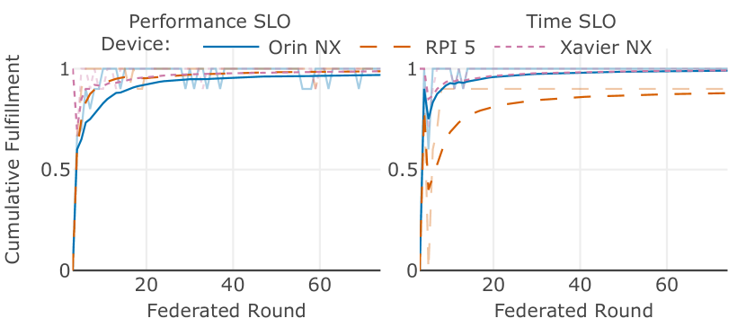
The next experiment focused on inspecting the ability of AIF agents to adapt to the resources available to the agents located at the edge devices and aligning them with the SLOs set. For the experiments, three edge devices (Raspberry Pi 5, Nvidia Orin NX, and Nvidia Xavier NX) were used as separate federated clients and were tasked to participate in the FL for 75 epochs, while a Raspberry Pi 4 device served as the FL orchestrator. No data drifts were introduced in this experiment. Due to the differences in resources, it was expected that agents would prefer different configurations under the same target SLOs. The comparison of SLO fulfillment across various devices is shown in Figure 12, and mean EFE is shown in Figure 13.

Figure 12: Mean SLOs fulfillment for different devices. Time SLO: 2 seconds, performance SLO: 97%

Figure 13: Mean EFE for different devices

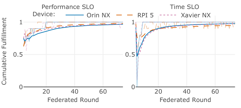
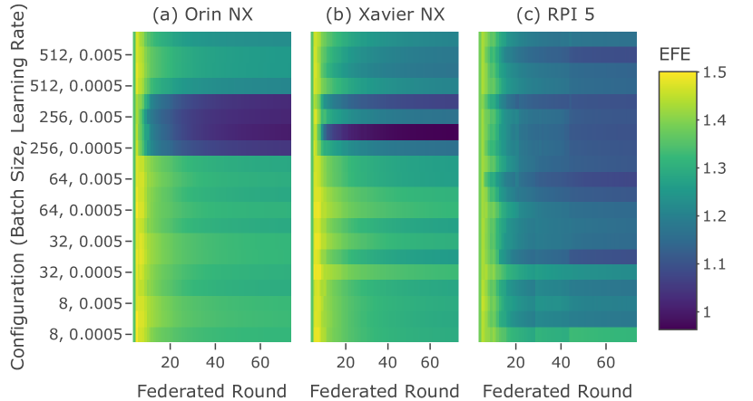
It is shown that all devices manage to fulfill the set SLOs. It is also worth noting that Raspberry Pi 5 managed to fulfill performance SLO slightly faster than devices that used GPU but occasionally struggled to maintain flawless time SLO fulfillment. When looking at mean EFE, it is clear that in order to better utilize its cores (as there is no GPU), Raspberry Pi can successfully employ a vast range of configurations due to the small size of the model (64 and 32 units in 2 layers), while devices with GPU choose bigger batch sizes to better utilize their parallelization capabilities.

To further inspect the adaptability of agents to different combinations of tasks, available resources, and set SLOs, the experiment was conducted with the same set of devices but with a wider neural network (5120 and 512 units compared to 64 and 32 used in the previous experiment). The time SLO was adjusted to 15 seconds. This change was introduced to give GPU-empowered devices an advantage over Raspberry Pi 5. The resulting SLOs fulfillment is shown in Figure 14 and mean EFE is shown in Figure 15. The performance SLO fulfillment at the final FL round was 96.9% for Orin NX and 98.7% for RPI 5 and Xavier NX, while the time SLO was 99% for Nvidia devices and 87.8% for RPI 5.

Figure 14: Mean SLOs fulfillment for different devices with a wider network. Time SLO: 15 seconds, performance SLO: 97%

Figure 15: Mean EFE for different devices and wider network

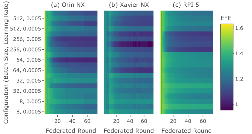
Here the change in the model architecture impacted the optimal configuration choice for Raspberry Pi 5. As seen from the mean EFE, the batch size had to be increased to 256 to fit into the time and performance SLOs, while Nvidia devices utilized a more comprehensive range of configurations.

The evaluation shows the potential of AIF agents in detecting the changes in the environment and the ability to initiate system re-configuration with no human supervision. However, the SLO fulfillment is not perfect. Two main explanations were identified up until now: (1) “unsupervised” BN structure learning using Hill Climb Search may struggle to discover meaningful causal relationships when limited data is available [22], (2) in the absence of observations with both SLOs fulfilled, an agent may either stuck in forever exploring state or stick to the strategy that guarantees at least one SLO fulfillment and focus on exploiting sub-optimal behavior.

VI Related Work

We identified three topics within related work: SLO fulfillment through dynamic adaptations in distributed computing systems, applications of the AIF framework, and optimization techniques in FL.

VI-A Optimization in Federated Learning

Optimizing FL workflows is important for minimizing the time-to-accuracy of model training [23]. In that context, Kundroo et al. [9] proposed FedHPO, a federated optimization algorithm that accelerates each client’s training by modifying its hyperparameters, such as learning rate or epochs.

Furthermore, several studies have focused on multi-objective optimization in FL. One possible approach is optimizing neural network models instead of client-specific hyperparameter optimization [24, 25]. Additionally, a significant number of existing research focuses on optimizing client selection or clustering instead of adjusting the parameters of individual clients to reach multi-dimensional goals [26, 27, 28].

Therefore, existing work on optimization in FL does not consider changing environments and lifelong FL scenarios or lacks individual clients’ hyperparameter tuning in general, which is crucial for pervasive applications.

VI-B Dynamic Adaptation for SLO Fulfillment

There exist multiple approaches that aim to combine SLOs with dynamic processing requirements: Zhang et al. [29] presented Octopus – the framework that finds optimal services configurations in multi-tenant edge computing scenarios. Octopus predicts SLO fulfillment of two variables based on a deep neural network. Shubha et al. [8] presented AdaInf, which detects SLO violations of a GPU scheduling task whenever variable drifts occur. Through AdaInf, it is possible to find SLO-fulfilling resource allocations between model training and inference.

VI-C AIF Applications

The cases in which AIF was used to dynamically support computing systems are mainly focused on robotics; Oliver et al. [30] give a comprehensive overview of how AIF allows (robotic) systems to act under uncertainty. Nevertheless, the application of AIF extends to continuous stream processing systems, such as provided by Sedlak et al. [6, 7], which uses a wide set of processing metrics as sensory observations. Actions taken by the processing system were elastic adaptations, e.g., scaling resources or quality, allowing to empirically find system configurations that fulfill SLOs.

Proved useful for ensuring the adaptability of robotic and stream processing systems, AIF could address the existing research gap in optimizing dynamic pervasive FL systems.

VII Conclusion

This work presented AIF agents that are able to adaptively change their behavior in response to dynamic environments. We evaluated the proposed AIF agents in lifelong heterogeneous FL, utilizing a set of both dynamic data and diverse devices. We showed that AIF agents are able to fulfill competing SLOs and unfolded the behaviors of agents and intricate connections between the defined SLOs and strategies for fulfilling them.

Future work can further expand the usage of the active inference framework to orchestrate distributed learning systems, for instance, by fulfilling system-level SLOs, such as fairness of participation or global model performance. Enhancements of the current method can improve the ability of the agents to find causal dependencies in limited data, making them more robust, targeting the limitations of the discrete BN, introducing temporal dependencies to capture the environmental dynamics more precisely, and providing more nuanced SLOs specifications to enable tracking SLOs in a range.

References

- [1] S. Dustdar, V. Casamayor Pujol, and P. K. Donta, “On Distributed Computing Continuum Systems,” IEEE Transactions on Knowledge and Data Engineering, vol. 35, no. 4, pp. 4092–4105, Apr. 2023.
- [2] T. Rausch, W. Hummer, C. Stippel, S. Vasiljevic, C. Elvezio, S. Dustdar, and K. Krösl, “Towards a platform for smart city-scale cognitive assistance applications,” in 2021 IEEE Conference on Virtual Reality and 3D User Interfaces Abstracts and Workshops (VRW), 2021, pp. 330–335.
- [3] M. Aboualola, K. Abualsaud, T. Khattab, N. Zorba, and H. S. Hassanein, “Edge technologies for disaster management: A survey of social media and artificial intelligence integration,” IEEE Access, vol. 11, pp. 73 782–73 802, 2023.
- [4] S. Deng, H. Zhao, W. Fang, J. Yin, S. Dustdar, and A. Y. Zomaya, “Edge intelligence: The confluence of edge computing and artificial intelligence,” IEEE Internet of Things Journal, vol. 7, no. 8, pp. 7457–7469, 2020.
- [5] A. Furtuanpey, P. Raith, and S. Dustdar, “Frankensplit: Efficient neural feature compression with shallow variational bottleneck injection for mobile edge computing,” IEEE Transactions on Mobile Computing, pp. 1–17, 2024.
- [6] B. Sedlak, V. C. Pujol, P. K. Donta, and S. Dustdar, “Equilibrium in the Computing Continuum through Active Inference,” Future Generation Computer System, 2024.
- [7] B. Sedlak, V. C. Pujol, A. Morichetta, P. K. Donta, and S. Dustdar, “Adaptive Stream Processing on Edge Devices through Active Inference,” Sep. 2024, arXiv:2409.17937 [cs].
- [8] S. S. Shubha and H. Shen, “AdaInf: Data Drift Adaptive Scheduling for Accurate and SLO-guaranteed Multiple-Model Inference Serving at Edge Servers,” in Proceedings of the ACM SIGCOMM 2023 Conference, ser. ACM SIGCOMM ’23. New York, NY, USA: Association for Computing Machinery, Sep. 2023, pp. 473–485.
- [9] M. Kundroo and T. Kim, “Federated learning with hyper-parameter optimization,” Journal of King Saud University - Computer and Information Sciences, vol. 35, no. 9, p. 101740, 2023.
- [10] A. L. Suárez-Cetrulo, D. Quintana, and A. Cervantes, “A survey on machine learning for recurring concept drifting data streams,” Expert Systems with Applications, vol. 213, p. 118934, 2023.
- [11] E. Jothimurugesan, K. Hsieh, J. Wang, G. Joshi, and P. B. Gibbons, “Federated learning under distributed concept drift,” in Proceedings of The 26th International Conference on Artificial Intelligence and Statistics, ser. Proceedings of Machine Learning Research, F. Ruiz, J. Dy, and J.-W. van de Meent, Eds., vol. 206. PMLR, 25–27 Apr 2023, pp. 5834–5853.
- [12] S. Nastic, A. Morichetta, T. Pusztai, S. Dustdar, X. Ding, D. Vij, and Y. Xiong, “Sloc: Service level objectives for next generation cloud computing,” IEEE Internet Computing, vol. 24, no. 3, pp. 39–50, 2020.
- [13] V. Casamayor Pujol, B. Sedlak, Y. Xu, P. K. Donta, and S. Dustdar, “Invited paper: Deepslos for the computing continuum,” in Proceedings of the 2024 Workshop on Advanced Tools, Programming Languages, and PLatforms for Implementing and Evaluating Algorithms for Distributed Systems, ser. ApPLIED’24. New York, NY, USA: Association for Computing Machinery, 2024, p. 1–10.
- [14] K. Friston, J. Kilner, and L. Harrison, “A free energy principle for the brain,” Journal of physiology-Paris, vol. 100, no. 1-3, pp. 70–87, 2006.
- [15] K. J. Friston, M. J. Ramstead, A. B. Kiefer, A. Tschantz, C. L. Buckley, M. Albarracin, R. J. Pitliya, C. Heins, B. Klein, B. Millidge, D. A. Sakthivadivel, T. S. C. Smithe, M. Koudahl, S. E. Tremblay, C. Petersen, K. Fung, J. G. Fox, S. Swanson, D. Mapes, and G. René, “Designing ecosystems of intelligence from first principles,” Collective Intelligence, vol. 3, no. 1, p. 26339137231222481, 2024. [Online]. Available: https://doi.org/10.1177/26339137231222481
- [16] T. Parr, G. Pezzulo, and K. J. Friston, Active inference: the free energy principle in mind, brain, and behavior. MIT Press, 2022.
- [17] D. Koller and N. Friedman, Probabilistic Graphical Models: Principles and Techniques - Adaptive Computation and Machine Learning. The MIT Press, 2009.
- [18] C. Heins, B. Millidge, D. Demekas, B. Klein, K. Friston, I. D. Couzin, and A. Tschantz, “pymdp: A python library for active inference in discrete state spaces,” Journal of Open Source Software, vol. 7, no. 73, p. 4098, 2022.
- [19] D. J. Beutel, T. Topal, A. Mathur, X. Qiu, J. Fernandez-Marques, Y. Gao, L. Sani, H. L. Kwing, T. Parcollet, P. P. d. Gusmão, and N. D. Lane, “Flower: A friendly federated learning research framework,” arXiv preprint arXiv:2007.14390, 2020.
- [20] Ankur Ankan and Abinash Panda, “pgmpy: Probabilistic Graphical Models using Python,” in Proceedings of the 14th Python in Science Conference, Kathryn Huff and James Bergstra, Eds., 2015, pp. 6 – 11.
- [21] J. Montiel, M. Halford, S. M. Mastelini, G. Bolmier, R. Sourty, R. Vaysse, A. Zouitine, H. M. Gomes, J. Read, T. Abdessalem, and A. Bifet, “River: machine learning for streaming data in python,” J. Mach. Learn. Res., vol. 22, no. 1, jan 2021.
- [22] N. K. Kitson, A. C. Constantinou, Z. Guo, Y. Liu, and K. Chobtham, “A survey of Bayesian Network structure learning,” Artificial Intelligence Review, vol. 56, no. 8, pp. 8721–8814, Aug. 2023.
- [23] Z. Jiang, W. Wang, B. Li, and Q. Yang, “Towards efficient synchronous federated training: A survey on system optimization strategies,” IEEE Transactions on Big Data, vol. 9, no. 2, pp. 437–454, 2022.
- [24] H. Zhu and Y. Jin, “Multi-objective evolutionary federated learning,” IEEE transactions on neural networks and learning systems, vol. 31, no. 4, pp. 1310–1322, 2019.
- [25] G. Paragliola, “Evaluation of the trade-off between performance and communication costs in federated learning scenario,” Future Generation Computer Systems, vol. 136, 06 2022.
- [26] M. Badar, S. Sikdar, W. Nejdl, and M. Fisichella, “Fairtrade: Achieving pareto-optimal trade-offs between balanced accuracy and fairness in federated learning,” Proceedings of the AAAI Conference on Artificial Intelligence, vol. 38, no. 10, pp. 10 962–10 970, Mar. 2024.
- [27] A. Lackinger, P. A. Frangoudis, I. Čilić, A. Furutanpey, I. Murturi, I. P. Žarko, and S. Dustdar, “Inference load-aware orchestration for hierarchical federated learning,” in 2024 IEEE 49th Conference on Local Computer Networks (LCN), 2024, pp. 1–9.
- [28] S. Yan, P. Zhang, S. Huang, H. Sun, Y. Zhang, and A. Tolba, “Node selection algorithm for federated learning based on deep reinforcement learning for edge computing in iot,” Electronics, vol. 12, p. 2478, 05 2023.
- [29] Z. Zhang, Y. Zhao, and J. Liu, “Octopus: SLO-Aware Progressive Inference Serving via Deep Reinforcement Learning in Multi-tenant Edge Cluster,” in Service-Oriented Computing, Cham, 2023.
- [30] G. Oliver, P. Lanillos, and G. Cheng, “An Empirical Study of Active Inference on a Humanoid Robot,” IEEE Transactions on Cognitive and Developmental Systems, vol. 14, no. 2, pp. 462–471, Jun. 2022.