Fair Decentralized Learning

Abstract

Decentralized learning (DL) is an emerging approach that enables nodes to collaboratively train a machine learning model without sharing raw data. In many application domains, such as healthcare, this approach faces challenges due to the high level of heterogeneity in the training data’s feature space. Such feature heterogeneity lowers model utility and negatively impacts fairness, particularly for nodes with under-represented training data. In this paper, we introduce Facade, a clustering-based DL algorithm specifically designed for fair model training when the training data exhibits several distinct features. The challenge of Facade is to assign nodes to clusters, one for each feature, based on the similarity in the features of their local data, without requiring individual nodes to know apriori which cluster they belong to. Facade (1) dynamically assigns nodes to their appropriate clusters over time, and (2) enables nodes to collaboratively train a specialized model for each cluster in a fully decentralized manner. We theoretically prove the convergence of Facade, implement our algorithm, and compare it against three state-of-the-art baselines. Our experimental results on three datasets demonstrate the superiority of our approach in terms of model accuracy and fairness compared to all three competitors. Compared to the best-performing baseline, Facade on the CIFAR-10 dataset also reduces communication costs by 32.3% to reach a target accuracy when cluster sizes are imbalanced.

I Introduction

DL is a collaborative learning approach that enables nodes to train a machine learning (ML) model without sharing their private datasets with other nodes [1]. In each round of decentralized learning (DL), nodes first locally train their model with their private datasets. According to a given communication topology, updated local models are then exchanged with neighbors and aggregated by each node. The aggregated model is then used as the starting point for the next round. This process repeats until model convergence is reached. Popular DL algorithms include D-PSGD [1], GL [2], and EL [3].

Nodes participating in DL are likely to own data with differing feature distributions [4]. For example, in a healthcare scenario, feature heterogeneity may arise due to differences in data acquisition, type of medical devices used, or patient demographics [5, 6]. Consider a network of hospitals that aims to train an advanced tumor detection model with DL. In this scenario, two different brands of scanners are available on the market, and each hospital uses one or the other. Due to slight differences in image acquisition processes, the feature distributions of the scanned images will vary between hospitals, most likely resulting in feature skew. For instance, features such as the image quality or contrast between the tumor and surrounding tissue may differ between the two types of scanners. If one brand of scanners is more widespread, standard DL approaches unfairly push the models towards the majority distribution. As a result, hospitals in the minority distribution exhibit low model utility, leading to diminished fairness.

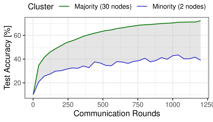
We highlight the extent of this fairness issue through an experiment in which we train an image classifier model (LeNet [7]) using D-PSGD in a 32-node network on the CIFAR-10 dataset [8]. For our experiment, we establish two clusters. The first cluster, the majority cluster, consists of 30 nodes, while the second cluster, the minority cluster, has two nodes. We ensure a uniform label distribution, with each node having an equal number of samples of each label. We create a feature distribution shift by turning the CIFAR-10 images for the nodes in the minority cluster upside down. Figure 1 shows the averaged test accuracy during training for the nodes in each cluster. We observe a significant accuracy gap of more than 30% between the two clusters, demonstrating that the model produced by decentralized parallel stochastic gradient descent (D-PSGD) is much less suitable for nodes in the minority cluster. This gap is often hidden in results when the global average test accuracy is reported, as this metric is biased towards the majority cluster due to their larger representation.

Figure 1: The test accuracy of a model trained with EL on CIFAR-10. Standard DL algorithms such as D-PSGD and EL results in significantly lower accuracy for the two nodes in the minority cluster compared to that of the nodes in the majority cluster.

As ML-based decision systems become more prevalent and are increasingly adopted, addressing fairness in DL and ML as a whole is critical [9]. These systems must actively mitigate biases that disproportionately harm minority groups [10]. In our work, we emphasize that differences in feature distribution should not degrade the prediction quality for nodes that have equally contributed to the learning process. This is especially crucial in high-stakes domains like healthcare, where the decisions made by ML models can have significant real-world consequences for individuals’ well-being.

To realize fairness in DL, we present Facade (FAir Clustered And Decentralized lEarning), a novel DL algorithm designed specifically for settings where training data exhibits two or more underlying features. In the presence of such feature heterogeneity, our approach ensures fair predictions across all nodes after model training. To our knowledge, we are the first to address both model utility and fairness in DL settings.

The main idea behind Facade is to group the nodes into clusters based on their feature skew. The number of clusters is a hyperparameter of Facade, is apriori defined, and should ideally match the number of distinct features in the data. However, as we will experimentally show in Section V-F, overestimating this number still yields good model accuracy. To enhance fairness, nodes specialize their models on the feature skew of their cluster while still collaborating with nodes outside their cluster to achieve good model utility across clusters. This collaboration dynamic allows nodes in a minority cluster to maintain specialized models that perform well on their data while also benefiting from the data of nodes in a majority cluster. Since the data in DL is private and cannot be shared, the key challenge lies in clustering the nodes as part of the DL training process in a fully decentralized manner.

Facade accomplishes this by splitting the models into two parts: (i) the common collaborative core and (ii) a specialized head. Each node maintains a single core and one head per cluster. At the start of each training round, each node chooses the head that, combined with the common core, shows the lowest training loss on the current batch of training samples. The chosen head is then trained along with the common core. The trained parts of the model are shared and aggregated, similar to DL algorithms like EL [3]. The dynamic topology used in EL provides better mixing of core and heads as the nodes aggregate models with varying nodes. The clustering process is emergent, , the nodes do not need to know which cluster they belong to. As the training progresses, nodes with similar feature distributions converge towards the same model head. This allows the head to specialize in the cluster’s feature distribution, resulting in better model utility and improved fairness of predictions across the network.

We implement Facade and conduct an extensive experimental evaluation with three datasets (CIFAR-10, Imagenette and Flickr-Mammals) and compare Facade to three state-of-the-art baselines (EL [3], DePRL [11] and DAC [12]). Our evaluation demonstrates that Facade consistently outperforms the baselines in terms of both test accuracy and fairness. For example, Facade achieves superior test accuracy for minority clusters, with up to 73.3% on the CIFAR-10 dataset, which outperforms the second-best algorithm, Facade, which reaches 68.4%. In addition, Facade is communication-efficient and requires 41.3% less communication volume than the EL baseline to reach a target accuracy of 63% on CIFAR-10, when cluster sizes are balanced. Our results underline the strength of Facade in delivering high model utility and fairness while also reducing communication overhead.

Contributions. Our work makes the following contributions:

1. We introduce a novel DL algorithm, named Facade, designed to address fairness concerns in the presence of feature heterogeneity (Section III). It ensures high fairness through emergent clustering, based on feature skew, and training specialized models with no additional communication overhead compared to standard DL algorithms such as D-PSGD.

2. We prove the convergence of Facade with an arbitrary number of feature distributions into which the population’s data is partitioned (Section IV). Our bounds depend on the number of nodes, the regularity and smoothness properties of local loss functions, the batch sizes used during local training, and the degree of the random graphs sampled at each communication round.

3. We experimentally evaluate Facade against three state-of-the-art baselines and datasets (Section V). Our results demonstrate that Facade results in high model utility for all clusters and excels at maintaining fairness, even for highly imbalanced scenarios where one group significantly outnumbers the other.

II Background and Preliminaries

We first introduce decentralized learning in Section II-A and then elaborate on the notion of fairness used in our work in Section II-B.

II-A DL

We consider a scenario where a group of nodes, denoted as $\mathcal{N}$, collaboratively train a ML model. This is commonly referred to as collaborative machine learning (CML) [13, 14]. Each node $i\in\mathcal{N}$ has its private dataset $D_{i}$, which is used for computing local model updates. The data from each node remains on the local device throughout the training process. The training aims to determine the model parameters $\theta$ that generalize well across the combined local datasets by minimizing the average loss over all nodes in the network.

DL [15, 1, 16] is a class of CML algorithms where nodes share model updates with neighboring nodes via a communication topology defined by an undirected graph $\mathcal{G}=(\mathcal{N},\mathcal{E})$. In this graph, $\mathcal{N}$ is the set of all nodes, and $(i,j)\in\mathcal{E}$ indicates an edge or communication link between nodes $i$ and $j$. In standard DL approaches, $\mathcal{G}$ is static but may also vary over time [17]. DL eliminates the need for centralized coordination, enabling each node to collaborate independently with its neighbors. This decentralized approach enhances robustness against single points of failure and improves scalability compared to alternative CML methods like federated learning (FL) [18].

Among the various algorithms, D-PSGD [1] is widely regarded as a standard for performing DL. In D-PSGD, each node $i$ starts with its loss function $f_{i}$, initializing its local model $\theta_{i}^{(0)}$ in the same way before executing the following steps:

1. Local training. For each round $0\leq t\leq T-1$ and each epoch $0\leq h\leq H-1$, initializing $\tilde{\theta}_{i}^{(t,0)}$ as $\theta_{i}^{(t)}$, node $i$ independently samples $\xi_{i}$ from its local dataset, computes the stochastic gradient $\nabla f_{i}(\tilde{\theta}_{i}^{(t,h)},\xi_{i})$, and updates its local model by setting $\tilde{\theta}_{i}^{(t,h+1)}\leftarrow\tilde{\theta}_{i}^{(t,h)}-\eta\nabla f_{i}(\tilde{\theta}_{i}^{(t,h)},\xi_{i})$, where $\eta$ represents the learning rate.

2. Model exchange. Node $i$ sends $\tilde{\theta}_{i}^{(t,H)}$ to its neighbors and receives $\tilde{\theta}_{j}^{(t,H)}$ from each neighboring node $j$ in $\mathcal{G}$.

3. Model aggregation. Node $i$ combines the model parameters received from its neighbors along with its own using a weighted aggregation formula: $\theta_{i}^{(t+1)}=\sum_{\{j:(i,j)\in\mathcal{E}\}\cup\{i\}}w_{ji}\tilde{\theta}_{j}^{\left(t,H\right)}$, where $w_{ji}$ is the $(j,i)^{\operatorname{th}}$ element of the mixing matrix $W$. A typical strategy is to aggregate the models with uniform weights from all neighbors, including the local model.

Upon completing $T$ rounds, node $i$ adopts the final model parameters $\theta_{i}^{(T)}$, concluding the DL training process. The pseudocode for D-PSGD is included in Appendix B.

II-B Fairness in Collaborative Machine Learning

With the recent increase in focus on building ethical ML models, formally ensuring the fairness of such models during or after training has become an important research challenge [19]. In the context of CML, various methods for quantifying and establishing fairness during model training have been explored from a variety of perspectives [20, 21, 22].

DP [23] is one of the most popular notions of group fairness used in ML to quantify the presence of bias of any subgroup of the participating data in the outcome of the trained model [24, 25, 26]. It formally ensures that the different demographic groups present in a population (, based on gender or race) receive positive treatment with equal likelihood, , $\mathbb{P}[\hat{Y}=y|S=0]=\mathbb{P}[\hat{Y}=y|S=1]$ where $\hat{Y}$ denotes the variable representing the decision (label) predicted by the model for a certain input, $y$ is the corresponding positive decision, and $S=0$ and $S=1$ denote the clusters where the sensitive attributes of the input come from (, representing the majority and the minority in the population).

To quantify the overall fairness of a ML algorithm trained for classification tasks w.r.t. demographic parity (DP) across all classes, we consider the sum of the absolute difference in DP across all possible labels [27, 28]. In other words, setting $\mathcal{Y}$ as the space of all possible labels that can be predicted, the overall DP across all classes ensured by the algorithm is given as:

$$\sum_{y\in\mathcal{Y}}\left\lvert\mathbb{P}[\hat{Y}=y|S=0]-\mathbb{P}[\hat{Y}=y|S=1]\right\rvert.$$ (1)

EO [24] is another widely used metric for group fairness in decision-making algorithms and classification-based ML [26, 28]. While the high-level goal of the equalized odds (EO) fairness metric is also to ensure that a model performs equally well for different groups, it is stricter than DP because it requires that the model’s predictions are not only independent of sensitive group membership but also that groups have the same true and false positive rates. This distinction is crucial because a model could achieve DP, , its predictions could be independent of sensitive group membership but still generate more false positive predictions for one group versus others. Formally, an algorithm satisfies EO if $\mathbb{P}[\hat{Y}=y|Y=y,S=1]-\mathbb{P}[\hat{Y}=y|Y=y,S=0]$, where, in addition to $\hat{Y}$ and $S$ as described above, $Y$ is the target variable denoting the ground truth label of an associated input. Similar to measuring the overall DP of a classification-based learning algorithm as given by Equation 1, the overall EO achieved by the algorithm across all classes is measured as the sum of the absolute differences in the EO across every possible label, ,

$$\sum_{y\in\mathcal{Y}}\left\lvert\mathbb{P}[\hat{Y}=y|Y,S=1]-\mathbb{P}[\hat{Y}=y|Y,S=0]\right\rvert.$$ (2)

In this work, we quantify the fairness guarantees of Facade and baseline approaches by evaluating both the DP and EO metrics across various learning tasks (also see Section V-D). Referring to the healthcare example presented in Section I, our goal is to ensure that under Facade, patients receive diagnoses of equal quality, , the model predicting whether a tumor is malignant or benign based on medical images, regardless of the brand of scanner used to obtain those images. In other words, Facade aims to ensure that, under formal standards of DP and EO, the diagnosis predicted by the model, , $\hat{Y}$ in the above definitions, is independent of any potential bias in the feature distribution of the images. Such biases may arise due to differences in the technical specifications of the scanners, causing the emergence of majority and minority groups ($S$ in the above definitions).

Figure 2: The different operations during a training round in Facade, from the perspective of node $N_{i}$.

III Design of Facade

Our work addresses fairness issues in DL due to potential bias in data features among nodes belonging to majority groups. We design Facade to operate within a permissioned network environment where membership is regulated. This assumption aligns with the notion that DL is often employed in enterprise contexts, where network access is typically restricted [29]. Examples of such environments include hospitals collaborating on DL tasks [30]. In permissioned networks, all nodes are verified entities with established identities. Therefore, we do not address threats in open networks, such as Sybil attacks [31], which fall outside the scope of this work. Additionally, we assume that nodes in Facade execute the algorithm correctly, and we consider issues like privacy or poisoning attacks beyond our scope. In line with related work in this domain, Facade is a synchronous learning system where communication and computations happen in discrete steps and rounds. Finally, Facade leverages a dynamic topology approach where the communication topology changes each round [3]. Refreshing this topology can be achieved by having nodes participate in topology construction using a decentralized peer-sampling service [32, 33].

In the following, we first explain the high-level operations of Facade in Section III-A. We then provide a formal, detailed algorithm description in the remaining subsections.

III-A Facade in a nutshell

We visualize the workflow of Facade in Figure 2. The underlying idea behind Facade is to maintain $k$ model heads per node, one for each cluster. Specifically, each model is split into a core and $k$ heads. In practice, the model heads are the final few layers of the neural network. These model heads can then effectively capture the unique variations of features across clusters. Thus, each node stores $k$ versions of the same head with different parameters, unlike other DL methods that only keep one model core and head in memory.

At the start of each round, the communication topology is first randomized (step 1 in Figure 2). Topology randomization in Facade is important to ensure good performance as otherwise nodes could become stuck with sub-optimal neighbors. Each node $n$ then receives model cores and heads from its neighbors and aggregates these received model cores and corresponding model heads (step 2). Specifically, if a node $n$ receives a head $h_{i}$, $n$ will aggregate $h_{i}$ with its own $i^{th}$ head. Furthermore, the core is always aggregated. Each node $n$ then evaluates the training loss on its mini-batch of training samples, using the model core and for each of the local model heads (step 3). $n$ then selects the model head with the lowest training loss and trains it, together with the model core (step 4). Finally, $n$ sends the updated model core and head to its neighbors in the communication topology (step 5). This process repeats until the model has converged.

A key benefit of Facade is that no explicit clustering is required: nodes are not pre-assigned to specific clusters before the training process. Instead, nodes in Facade are implicitly clustered through dynamic head evaluation and selection. This procedure allows the clustering to evolve dynamically, enabling nodes to detect similarities with others as models become more specialized and accurate.

III-B Notations

Let $\mathcal{N}=\{N_{1},\ldots N_{n}\}$ be the set of all nodes in the network and let $Z_{i}\in\mathcal{Z}$ denote the local dataset of $N_{i}$ for each $i\in[n]$. We consider a setting where the features of the data held by each of the $n$ nodes are partitioned into $k$ distinct distributions, $\mathcal{D}_{1},\ldots,\mathcal{D}_{k}$, for some $k\leq n$. In other words, we assume that for every $i\in[n]$, there exists a unique $j_{i}\in[k]$ such that the datapoints in $Z_{i}$ are sampled from $\mathcal{D}_{j_{i}}$ and we refer to $j_{i}$ as the true cluster ID of $N_{i}$. For every $j\in[k]$, let $S^{*}_{[j]}\subseteq\mathcal{N}$ denote the set of nodes whose true cluster identity is $j$, , $S^{*}_{[j]}=\{N_{i}\in\mathcal{N}\colon\,Z_{i}\sim\mathcal{D}_{j}\}$, and we refer to $S^{*}_{[j]}$ as the $j$’th cluster of the network.

III-C Problem formulation

For each $i\in[n]$, let $f_{i}:\mathbb{R}^{d}\mapsto\mathbb{R}$ be the loss function of $N_{i}$. In practice, nodes sample a finite subset of their personal data set, referred to as a batch, for their local training. Let $\xi^{(t)}_{i}\subseteq Z_{i}$ represent the batch sampled in round $t$ by $N_{i}$, independent of the past and other nodes; we assume that the batch size $B=|\xi^{(t)}_{i}|$ remains constant for all nodes in every round. Thus, for every $i\in[n]$, $f_{i}(\theta,\xi_{i}^{(t)})=\frac{1}{B}\sum_{z\in\xi^{(t)}_{i}}f_{i}(\theta,z)$ is the empirical loss evaluated by $N_{i}$ on batch $\xi^{(t)}_{i}$ for model $\theta$.

We recall that Facade achieves fairness in collaboratively trained models through clustering in a decentralized framework, accounting for the heterogeneous feature distribution of data across nodes. This is ensured by the fact that Facade trains models tailored for each cluster specific to the feature distribution of their data. Hence, for every $j\in[k]$, the nodes in $S^{*}_{[j]}$ seek to minimize the average population loss of the $j$’th cluster given by $F^{[j]}=\frac{1}{|S^{*}_{[j]}|}\sum_{i^{\prime}:N_{i^{\prime}}\in S^{*}_{j}}f_{i^{\prime}}$. Thus, the training objective of Facade is to find an optimal model for each cluster that minimizes the corresponding population loss, which can be formally expressed as:

$$\forall\,j\in[k]:\theta^{*}_{[j]}=\operatorname{argmin}_{\theta\in\mathbb{R}^{d}}F^{[j]}(\theta)$$

$$\text{where }F^{[j]}(\theta)=\frac{1}{|S^{*}_{[j]}|}\sum_{i^{\prime}:N_{i^{\prime}}\in S^{*}_{j}}f_{i^{\prime}}(\theta,Z_{i^{\prime}})\;\;\;\forall j\in[k].$$

III-D Detailed algorithm description

In each round $t$, the nodes furnish a randomized $r$-regular undirected topology $\mathcal{G}_{t}=(\mathcal{N},\mathcal{E}_{t})$ where $\mathcal{E}_{t}$ is the set of all edges, denoting communication between a pair of nodes, formed independently of the previous rounds. Let $\mathcal{V}_{i}^{(t)}\subset\mathcal{N}$ be the set of all neighbors of $N_{i}$ for every $i\in[n]$.

For every $i\in[n]$, $j\in[k]$, and in any round $t$, let $\theta^{(t)}_{i}$ be $N_{i}$’s local model divided into a head $h^{(t)}_{i}$ and a core $\phi^{(t)}_{i}$ and we write $\theta^{(t)}_{i}=h^{(t)}_{i}\circ\phi^{(t)}_{i}$. In round $t=0$, Facade starts by initializing $k$ models that are shared with every node, where each model consists of a cluster-specific unique head and a common core. During each round, every node receives models (divided into head and core) from their neighbors, aggregates all the cores with its own, and performs a cluster-wise aggregation of the heads. Each node then concatenates the aggregated core with the $k$ (cluster-wise) aggregated heads to form $k$ different models and identifies the one that results in the least loss with its own data. It then performs the SGD steps on that model before sharing the locally optimized model and its corresponding cluster ID with its neighbors.

For every $i\in[n]$, $j\in[k]$, and in any round $t$, set $S^{(t)}_{[j]}\subseteq\mathcal{N}$ to be the set of all nodes reporting their cluster ID as $j$ in round $t$. Then, let $\bar{\theta}^{[j](t)}$ be the global aggregated model for the $j$’th cluster given by $\bar{\theta}^{[j](t)}=\frac{1}{|S^{(t)}_{[j]}|}\sum_{i\in S^{(t)}_{[j]}}\theta^{(t)}_{i}$ and let $\bar{\theta}_{i}^{[j](t)}=\bar{h}^{[j](t)}_{i}\circ\bar{\phi}^{(t)}_{i}$ be the aggregate of the models with the cluster identity $j$ received by $N_{i}$ where $h^{[j](t)}_{i}$ and $\phi^{(t)}_{i}$ are computed as:

$$\bar{\phi}^{(t)}_{i}=\frac{1}{|\hat{\mathcal{V}}_{i}^{(t)}|}\sum_{i^{\prime}\in\hat{\mathcal{V}}_{i}^{(t)}}\phi_{i^{\prime}}^{(t)}\text{ and }$$ (3)

$$\bar{h}^{[j](t)}_{i}=\frac{1}{|S^{(t)}_{j}\cap\hat{\mathcal{V}}_{i}^{(t)}|}\sum_{i^{\prime}:N_{i^{\prime}}\in S^{(t)}_{j}\cap\hat{\mathcal{V}}_{i}^{(t)}}h^{(t)}_{i^{\prime}},$$ (4)

where $$\hat{\mathcal{V}}_{i}^{(t)}=\mathcal{V}_{i}^{(t)}\cup\{N_{i}\}$$.

The workflow of the Facade algorithm can formally be described as follows.

The Facade Algorithm

Round $T\geq t\geq 0$ in Facade consists of the following three steps.

1. Randomized topology. The randomized communication topology $\mathcal{G}=(\mathcal{N},\mathcal{E}_{t})$ is established.

2. Local steps. For all $i\in[n]$ and in any round $t$:

   1. Receive models. $N_{i}$ receives $\theta_{i^{\prime}}^{(t)}=h_{i}^{(t)}\circ\phi_{i}^{(t)}$ and the corresponding cluster IDs from each $i^{\prime}\in\mathcal{V}_{i}^{(t)}$.

   2. Cluster-wise aggregation. $N_{i}$ aggregates the cores and performs a cluster-wise aggregation of the heads as given by Equations 3 and 4, respectively, to obtain $\bar{\theta}_{i}^{[j](t)}=\bar{h}_{i}^{(t)}\circ\bar{\phi}_{i}^{(t)}$ for every cluster $j\in[k]$.

   3. Cluster identification. $N_{i}$ obtains the cluster ID that gives the least loss on its local data.

      $$\hat{j}^{(t)}_{i}=\operatorname{argmin}_{j\in[k]}\nabla f_{i}(\bar{\theta}_{i}^{[j](t)},\xi^{(t)}_{i})$$

   4. Local training. Let $\tilde{\theta}_{i}^{[\hat{j}_{i}^{(t)}](t,0)}=\bar{\theta}_{i}^{[\hat{j}_{i}^{(t)}](t)}$.

      $$\text{For }h\leq H-1\colon$$

      $$\tilde{\theta}_{i}^{[\hat{j}_{i}^{(t)}](t,h+1)}=\tilde{\theta}_{i}^{[\hat{j}_{i}^{(t)}](t,h)}-\eta\nabla f_{i}(\tilde{\theta}_{i}^{[\hat{j}_{i}^{(t)}](t,h)},\xi^{(t)}_{i}),$$

      where $\nabla f_{i}(\tilde{\theta}_{i}^{[\hat{j}_{i}^{(t)}](t,h)},\xi^{(t)}_{i})$ is the stochastic gradient of $f_{i}$ computed on batch $\xi^{(t)}_{i}$, $\eta>0$ is the learning rate, and $H$ is the number of local SGD steps performed.

3. Communication step. For every $i\in[n]$, set $\theta_{i}^{(t+1)}=\tilde{\theta}_{i}^{[\hat{j}_{i}^{(t)}](t,H)}$ and share $(\theta_{i}^{(t+1)},\hat{j}^{(t)}_{i})$ with the nodes in $\mathcal{V}_{i}^{(t)}$.

III-E Discussion

We now discuss various properties of the Facade algorithm.

Random Topologies. We randomize the communication topology for the following two reasons. First, it has been demonstrated that altering random communication topologies leads to faster model convergence than traditional DL approaches that maintain a static, fixed topology throughout training [3]. Second, in Facade, dynamic topologies also prevent nodes in a cluster from becoming isolated due to initial neighbors from other clusters. By sampling random neighbors each round, an isolated node will likely eventually exchange models with nodes with similar data features.

Overhead. Compared to D-PSGD, Facade incurs some storage and compute overhead. The storage overhead stems from each node having to store $k$ model heads. However, since model heads generally consist of a very small number of parameters compared to the full model, the storage overhead of storing $k$ model heads is negligible. Furthermore, there is additional compute overhead as each node is required to compute $k$ training losses each training round, one for each model head. However, this overhead is also manageable since one can store the output tokens of the model core and input these to each model head. Alternatively, the $k$ forward passes can also be computed in parallel.

Choice of $k$. As with many other clustering algorithms [34, 35], the number of clusters ($k$) is a hyperparameter, which should be estimated by the system designer beforehand. This value heavily depends on the application domain and characteristics of individual training datasets. We experimentally show in Section V-F that our algorithm performs well even if the chosen $k$ is not exactly equal to the true number of feature distributions in the network.

IV Theoretical analysis of convergence

We now theoretically analyze the convergence of the cluster-wise aggregated models under Facade. We begin by introducing some additional notation and outlining the assumptions we make, followed by deriving the intermediate results (Theorems 1 and 2) that lead to the final result (Corollary 3).

For every cluster $j\in[k]$, we assume the existence of an optimal model $\theta^{*}_{[j]}$ that minimizes the average loss of the nodes in $S^{*}_{[j]}$. In order to theoretically analyze the convergence of Facade, in addition to the notations introduced in Section III-B, we introduce the following additional terms. For every $i\in[n]$, $j\in[k]$, and in any round $t$, let $F^{[j](t)}_{i}=\frac{1}{|S^{(t)}_{j}\cap\hat{\mathcal{V}}_{i}^{(t)}|}\sum_{i^{\prime}\in S^{(t)}_{j}\cap\hat{\mathcal{V}}_{i}^{(t)}}f_{i^{\prime}}$ be the average loss of the neighbors of $N_{i}$ who report their cluster ID as $j$ in round $t$ and we refer to this quantity as the local population loss in the for the $j$’th cluster in the neighborhood of $N_{i}$ in round $t$. Finally, for every $j\in[k]$, let $p_{[j]}=\frac{|S^{*}_{j}|}{n}$ denote the fraction of nodes belonging to cluster $j$ with $p=\min_{j\in[k]}\{p_{j}\}$ and let $\Delta$ denote the minimum separation between the optimal models of every cluster, , $\Delta=\min_{j\neq j^{\prime}}\norm{\theta^{*}_{[j]}-\theta^{*}_{[j^{\prime}]}}$.

We now proceed to study how the cluster identities reported by each node in every round of Facade correspond to their true cluster identities over time. In order to develop the theoretical analysis, we adhere to a standard set of assumptions which are widespread in related works [36, 37, 3, 38, 39]. In the interest of space, the proofs of all the theoretical results presented in this section are postponed to Appendix A.

Assumption 1.

For every $i\in[n]$, $j\in[k]$, and in round $t\geq 0$, the corresponding local population loss of the $j^{th}$ cluster in the neighborhood of $N_{i}$ in round $t$ is $\lambda$-convex and $L$-smooth. Formally, for every $\theta,\theta^{\prime}\in\mathbb{R}^{d}$, there exist constants $\lambda\geq 0$ and $L\geq 0$ such that:

$$F^{[j](t)}_{i}(\theta^{\prime})-F^{[j](t)}_{i}(\theta)$$

$$\geq\left\langle\nabla F^{[j](t)}_{i}(\theta),\,\theta^{\prime}-\theta\right\rangle+\frac{\lambda\norm{\theta^{\prime}-\theta}_{2}^{2}}{2}\text{ ($\lambda$-convexity) and}$$

$$\norm{\nabla F^{[j](t)}_{i}(\theta)-\nabla F^{[j](t)}_{i}(\theta^{\prime})}\leq L\norm{\theta-\theta^{\prime}}\text{ ($L$-smoothness)}.$$

Assumption 2.

For every $i\in[n]$ and in any round $t\geq 0$, the variances of $f_{i}$ and $\nabla f_{i}$ computed on batch $\xi_{i}^{(t)}\subset Z_{i}$, sampled according to $\mathcal{D}_{j_{i}}$, are bounded by $\sigma^{2}$ and $\nu^{2}$, respectively,

$$\mathbb{E}_{\xi_{i}\sim\mathcal{D}_{j_{i}}}\left[\left(f_{i}(\theta,\xi_{i}^{(t)})-F^{[j_{i}](t)}_{i}(\theta)\right)^{2}\right]\leq\sigma^{2}\text{ and}$$

$$\mathbb{E}_{\xi_{i}^{(t)}\sim\mathcal{D}_{j_{i}}}\left[\norm{\nabla f_{i}(\theta,\xi_{i}^{(t)})-\nabla F^{[j_{i}](t)}_{i}(\theta)}^{2}\right]\leq\nu^{2}.$$

In addition to Assumptions 1 and 2, we also assume some initialization conditions of Facade. These are consistent with the standard works on clustering-based personalized model training in FL [36].

Assumption 3.

For every cluster $j\in[k]$, we assume Facade to satisfy the following initialization conditions:

$$\norm{\bar{\theta}_{i}^{[j](0)}-\theta^{*}_{[j]}}\leq(\frac{1}{2}-\alpha)\sqrt{\frac{\lambda}{L}}\Delta,$$

$$\text{where $0\leq\alpha\leq\frac{1}{2}$},\,B\geq\frac{k\sigma^{2}}{\alpha^{2}\lambda^{2}\Delta^{4}},\,p\geq\frac{\log(nB)}{B},\text{ and}$$

$$\Delta\geq\bar{\mathcal{O}}\max\{(\alpha^{-2/5}B^{-1/5})\alpha^{-1/3}n^{-1/6}B^{-1/3}\}.$$

Theorem 1.

If Assumptions 1, 2 and 3 hold, choosing learning rate $\eta=1/L$, for a fixed node $N_{i}$, each cluster $j\in[k]$, and any $\delta\in(0,1)$, in every round $t>0$, we have with probability at least $(1-\delta)$:

$$\norm{\bar{\theta}_{i}^{[j](t+1)}-\theta^{*}_{[j]}}\leq(1-\frac{p\lambda}{8L})\norm{\bar{\theta}_{i}^{[j](t)}-\theta^{*}_{[j]}}+\epsilon_{0}$$

where $\epsilon_{0}\leq\frac{\nu}{\delta L\sqrt{pnB}}+\frac{\sigma^{2}}{\delta\alpha^{2}\lambda^{2}\Delta^{4}B}+\frac{\sigma\nu k^{3/2}}{\delta^{3/2}\alpha\lambda L\Delta^{2}\sqrt{n}B}$.

Theorem 2.

If Assumptions 1, 2 and 3 hold, choosing learning rate $\eta=1/L$, for each cluster $j\in[k]$ and in every round $t>0$, let the locally aggregated model for any cluster at each node be independent of each other. Then for any $\delta\in(0,1)$, we have with probability at least $(1-\delta)^{|S^{(t)}_{[j]}|}$:

$$\norm{\bar{\theta}^{[j](t+1)}-\theta^{*}_{[j]}}\leq(1-\frac{p\lambda}{8L})\norm{\bar{\theta}^{[j](t)}-\theta^{*}_{[j]}}+\epsilon_{0}$$

where $\epsilon_{0}\leq\frac{\nu}{\delta L\sqrt{pnB}}+\frac{\sigma^{2}}{\delta\alpha^{2}\lambda^{2}\Delta^{4}B}+\frac{\sigma\nu k^{3/2}}{\delta^{3/2}\alpha\lambda L\Delta^{2}\sqrt{n}B}$.

Finally, in order to derive the convergence analysis for each cluster, in every round $t>0$ and for each cluster $j\in[k]$, let the global aggregate model for cluster $j$ be given by $\theta^{[j](t)}=\frac{1}{|S^{(t)}_{[j]}|}\sum_{i:N_{i}\in S^{(t)}_{[j]}}\bar{\theta}_{i}^{[j](t)}$. The following result now helps us understand the cluster-wise convergence of the models under Facade.

Corollary 3.

If Assumptions 1, 2 and 3 hold, choosing learning rate $\eta=1/L$, for each cluster $j\in[k]$ and in every round $t>0$, let the locally aggregated model for any cluster at each node be pairwise independent of each other. Then for any $\delta\in(0,1)$ and any $\epsilon>0$, setting $\hat{T}=\frac{8L}{p\lambda}\log(\frac{2\Delta}{\epsilon})$, in any round $t\geq\hat{T}$ of Facade, we have with probability at least $(1-\delta)^{|S^{(t)}_{[j]}|}$:

$$\norm{\theta^{[j](t)}-\theta^{*}_{[j]}}\leq\epsilon$$

where $\epsilon\leq\frac{\nu kL\log(nB)}{p^{5/2}\lambda^{2}\delta\sqrt{nB}}+\frac{\sigma^{2}L^{2}k\log(nB)}{p^{2}\lambda^{4}\delta\Delta^{4}B}+\bar{\mathcal{O}}(\frac{1}{B\sqrt{n}})$.

Remark 1.

We note that, for any $i\in[n]$ and in each round $t$, as the degree of $N_{i}$ in the communication topology $\mathcal{G}_{t}$ increases, $F^{[j_{i}](t)}_{i}$ provides a better estimate of $F^{[j_{i}]}$, which consequently reduces the upper bounds of the variances of $f_{i}$ and $\nabla f_{i}$ (, $\sigma^{2}$ and $\nu^{2}$, respectively) under Assumption 2. This occurs because the local population loss in the neighborhood of $N_{i}$ for its true cluster ID $j_{i}$ becomes closer to the overall population loss for cluster $j_{i}$. Hence, from Corollary 3, observing that the convergence rates of the cluster-wise aggregated models are directly proportional to $\sigma^{2}$ and $\nu^{2}$, we conclude that as the degree of regularity of the communication topology increases, we expect faster convergence, with the extreme case of a fully connected topology converging at the same rate as in FL.

Theorem 2 essentially implies that, for each node, the cluster-wise aggregation of the model received from its neighbors probabilistically converges to the optimal model for the corresponding cluster, up to a small bounded error of $\epsilon_{0}$. Building on this result, Corollary 3 shows that for any arbitrary error $\epsilon$, there exists a round $\hat{T}$ such that, for every round $t\geq\hat{T}$, the difference between the cluster-wise aggregated model over the entire population and the optimal model for the corresponding cluster probabilistically becomes smaller than $\epsilon$. This, in turn, formally guarantees the convergence of Facade.

TABLE I: Summary of datasets and parameters used to evaluate Facade and DL baselines.

Dataset	Nodes	Model	Model Params.	Learning Rates
				EL	DAC	DePRL	Facade
CIFAR-10 [8]	32	CNN (LeNet [7])	120k	$\eta=0.05$	$\eta=0.005$	$\eta=0.01$	$\eta=0.01$
Imagenette [40]	24	CNN (LeNet [7])	250k	$\eta=0.001$	$\eta=0.001$	$\eta=0.0005$	$\eta=0.0003$
Flickr-Mammals [41]	16	ResNet8 [42]	310k	$\eta=0.1$	$\eta=0.3$	$\eta=0.1$	$\eta=0.3$

V Experimental Evaluation

We conduct an extensive experimental evaluation of Facade and explore its performance against related state-of-the-art DL algorithms. We implement Facade and baselines using the DecentralizePy framework [43] and open-source our code.

Our experiments answer the following six questions:

1. What is the per-cluster test accuracy for Facade and baselines when varying the cluster sizes (Section V-B)?

2. What is the fair accuracy for Facade and baselines when varying the cluster sizes (Section V-C)?

3. What is the fairness for Facade and baselines, in terms of DP and EO, when varying the cluster sizes (Section V-D)?

4. How does the communication cost to reach a fixed target accuracy of Facade compare to that of baselines (Section V-E?

5. What is the impact of wrongly estimating $k$ (Section V-F)?

6. How does Facade implicitly assign nodes to clusters (Section V-G)?

V-A Experimental setup

Datasets and Partitioning. Our experiments focus on supervised image classification as a universal task setting, which is in line with our baselines [3, 11, 12] and related work [36]. Specifically, we conduct our experiments on the CIFAR-10 [8], Flickr-Mammals [41] and Imagenette [40] datasets. The CIFAR-10 dataset is a widely-used image classification task, containing $50\,000$ images evenly divided among ten classes (with a resolution of 32x32 pixels). Imagenette is a subset of ten classes taken from Imagenet [44] with $9469$ images (with a resolution of 224x224 pixels) in total. Finally, the Flickr-Mammals dataset contains $48\,158$ images of $41$ different mammal species with varying resolution. Table I summarizes the used dataset and learning parameters.

To create an environment with clustered data with feature skew, we first uniformly partition each dataset into several smaller subsets, , each client has the same number of training samples from each class. We use uniform partitioning because our work aims to study fairness in networks with feature heterogeneity, not label skewness. Thus, the heterogeneity must be reflected in the feature composition of each cluster. To ensure feature heterogeneity, we randomly apply different rotations to the images of each cluster, ensuring that no two clusters share the same rotation. This is in line with related work [45, 36]. We note that this process maintains the same label distribution across clusters while introducing recognizable differences in feature compositions. Additionally, all nodes within the same cluster share a common test set with the same rotation as their training set, ensuring the test data has the same feature shift.

Cluster Configurations. To assess the fairness of Facade and baselines, we design experiments with multiple clusters with varying proportions. We keep the total number of nodes constant for all experiments while varying the cluster sizes. We demonstrate that, even when the minority group is heavily outnumbered by the majority group, Facade maintains a high accuracy for all clusters and significantly improves accuracy for the minority group compared to baseline algorithms.

Unless specified otherwise, we experiment with two clusters of varying sizes. For CIFAR-10, we consider three cluster configurations and $32$ nodes, with majority-to-minority ratios of 16:16, 24:8, and 30:2. For instance, for the 24:8 cluster configuration, 24 nodes have upright images, while the remaining $8$ nodes possess images that are rotated 180°. For Imagenette, we have $24$ nodes in total and consider cluster configurations with ratios of 12:12, 16:8, and 20:4. For Flickr-Mammals, we have $16$ nodes and consider two cluster configurations with ratios 8:8 and 14:2. While most of our experiments focus on a two-cluster setup, Facade can be applied to configurations with more than two clusters, as shown in Section V-F. Moreover, our convergence analysis (see Section IV) is carried out for an arbitrary number of clusters in the population.

Models. We use GN-LeNet for the CIFAR-10 experiments [41]. It has about 120k parameters, consisting of three convolution layers and one feed-forward layer. When training models with Facade, we designate the last fully connected layer as the head and use the rest of the model as the common core. We also use a LeNet model for Imagenette but adjust the model to accept images with a 64x64 pixel resolution. The resulting number of parameters of this model is about 250k. For Flickr-Mammals, we use a ResNet8 [42] model, with roughly 310k parameters, that accept 64x64 pixel images as input. Since this dataset is more challenging, we modify the head size of ResNet8 and include the last two basic blocks in the head, along with the final fully connected layer.

Baselines. We compare Facade against three related DL algorithms: EL [3], DePRL [11] and DAC [12]. EL is a state-of-the-art DL algorithm that leverages randomized communication to improve model convergence, and we have included it as a baseline since Facade also relies on communication with random nodes [3].

DePRL is a state-of-the-art personalized DL algorithm that allows each node to optimize its model head locally while sharing the core model through periodic communication and aggregation steps [11]. In contrast to Facade, DePRL uses a static communication topology and does not share the head with other nodes each communication round. Furthermore, DePRL focuses on dealing with label heterogeneity, whereas the focus of Facade is on feature heterogeneity instead.

We also compare against DAC, a state-of-the-art approach for personalized DL on clustered non-IID data [12]. This approach adapts the communication weights between nodes based on their data distributions, enhancing learning efficiency and performance in clustered settings. Like Facade, DAC utilizes a dynamic communication topology and has been tested on cluster configurations similar to our work. Finally, we remark that none of the selected DL baselines consider fairness, which is a unique contribution of our work.

Learning Parameters. We run each experiment for $T=1200$, $T=800$, and $T=1200$ communication rounds for the CIFAR-10, Imagenette, and Flickr-Mammals datasets, respectively. Each local training round features $\tau=10$ local steps with batch size $B=8$. For Flickr-Mammals, we increase the number of local steps to $\tau=40$. We use the SGD optimizer for Facade and all baselines and have independently tuned the learning rate for each learning task and baseline with a grid search. Table I summarizes these parameters. For Facade and baselines, we perform an all-reduce step in the final round [46], where all nodes share their models with everyone else and perform a final aggregation. Finally, we fix the communication topology degree to $4$ for Facade and baselines.

To evaluate the algorithms, we measure the test accuracy on the provided test sets every $80$ rounds. We also compute the relevant fairness metrics (DP and EO) of the final models with Equation 1 and Equation 2. In the main text, we provide experimental results for the CIFAR-10 and Imagenette datasets and complementary experimental results and plots for the Flickr-Mammals dataset in Appendix D.

(a) 16:16 cluster configuration

(b) 24:8 cluster configuration

(c) 30:2 cluster configuration

Figure 3: Average test accuracy for the nodes in the majority cluster (left) and those in the minority (right) obtained on CIFAR-10 ($\uparrow$ is better), for different cluster configurations.

(a) 12:12 cluster configuration

(b) 16:8 cluster configuration

(c) 20:4 cluster configuration

Figure 4: Average test accuracy for the nodes in the majority cluster (left) and those in the minority (right) obtained on Imagenette ($\uparrow$ is better), for different cluster configurations.

V-B Per-cluster test accuracy for varying cluster configurations

We analyze the per-cluster test accuracy for the CIFAR-10 and Imagenette datasets when varying the cluster size. Our goal is to analyze the performance of Facade and baselines when the minority group is increasingly outnumbered.

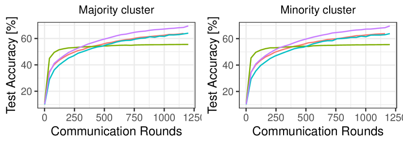
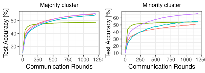
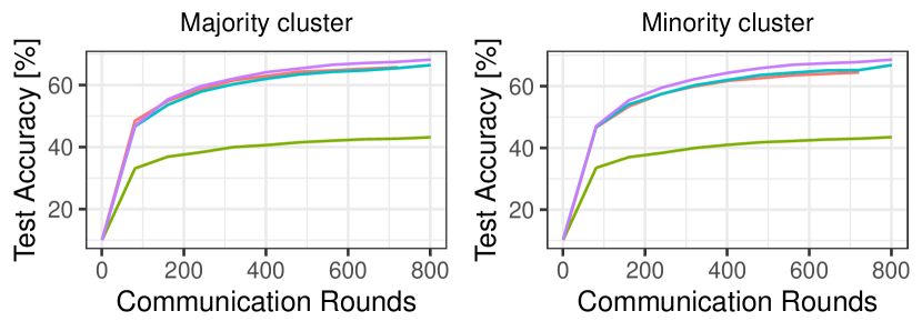
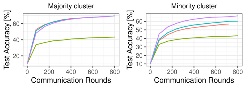
Figure 3 shows the average test accuracy for each cluster for the CIFAR-10 dataset as model training progresses for the three considered cluster configurations. The test accuracy of the majority and minority clusters is shown in the left and right columns, respectively. When both clusters are of equal size (Figure 3(a)), Facade attains higher model utility compared to baselines: 64.0% and 69.5% for EL and Facade, respectively, after $T=1200$. We attribute this gain to the management of multiple heads by Facade, which provides a greater capacity to adapt to variations in features across clusters. Generally, most of our baselines show reasonable performance with test accuracies around 63%, since there is enough data to find a good model that suits both clusters. We also observe that the attained accuracy of DePRL plateaus early in the training process. For all cluster configurations, we observe that Facade either outperforms or is at par with the baselines.

When considering the test accuracy of minority clusters (right column of Figure 3), we note that Facade consistently outperforms baselines and gives the minority groups a test accuracy that, for a fixed cluster configuration, is comparable to the one for the nodes in the majority cluster. When cluster configurations become more skewed (Figure 3(b) and Figure 3(c)), the attained test accuracy of EL drops significantly. This is because consensus-based methods like EL optimize for the data distribution of the majority cluster. Compared to other baselines, DePRL performs well in the 30:2 cluster configuration (Figure 3(c)) and reaches 55.4% test accuracy after $T=1200$. We attribute this performance to the specialization of model heads to the heterogeneous features. Nevertheless, Facade outperforms all baselines in terms of test accuracy of the minority cluster. In the 24:8 cluster configuration, Facade reaches 66.8% test accuracy compared to 54.8% test accuracy for EL. For the highly skewed cluster configuration of 30:2, Facade reaches 60.0% test accuracy compared to 52.5% test accuracy for DePRL. Facade thus demonstrates fair treatment to the minority group. The superior performance of Facade for the majority group is because the model heads are specialized for each cluster. This allows the model head to remain unaffected by the majority’s data distribution and to adapt specifically to the minority group’s data distribution. We also notice that for all cluster configurations baselines achieve higher accuracy on the majority group, which we believe is because this group has more data samples.

Figure 4 shows similar plots for the Imagenette dataset. We observe similar trends as in Figure 3: Facade shows comparable test accuracy for the nodes in the majority cluster and significantly higher test accuracy for nodes in the minority cluster. Figure 4(c) (right) shows that after $T=800$, Facade achieves 64.1% test accuracy compared to 56.1% test accuracy for EL. Finally, Figure 13 (in the appendix) shows that Facade also achieves a significant boost in model utility for the minority group in a 14:2 cluster configuration.

(a) CIFAR-10

(b) Imagenette

Figure 5: Highest observed fair accuracy for CIFAR-10 (top) and Imagenette (bottom), for varying cluster configurations and algorithms ($\uparrow$ is better).

V-C Fair accuracy for varying cluster configurations

We observe that the fairness metrics introduced in Section II-B primarily focus on ensuring that the model’s predictions are independent of the different clusters in the network. However, this overlooks the actual performance of the models, as a model that performs equally poorly across all groups could still receive a favorable fairness score. For example, a random model achieving merely $10\%$ accuracy on a ten-class dataset ($\sim$ random guessing) would exhibit the highest possible fairness under these metrics simply because there would be no performance disparity between the groups.

V-C1 Fair accuracy metric

In order to demonstrate a more comprehensive evaluation of the performance of Facade by considering both fairness and accuracy, we introduce the notion of fair accuracy. Reflecting to the issue illustrated in Figure 1, we recall that one of the primary motivations behind Facade is to reduce the performance gap between different clusters while maintaining high overall accuracy. We introduce the fair accuracy metric, which captures this by balancing the goal of achieving high overall accuracy while minimizing performance disparities between the clusters. For $\lambda\in[0,1]$, the normalized fair accuracy, denoted by $\operatorname{Acc}_{\operatorname{fair}}$, is defined as follows:

$$\operatorname{Acc}_{\operatorname{fair}}=\frac{\lambda\sum_{j\in[k]}\operatorname{Acc}_{j}}{k}+(1-\lambda)P,$$ (5)

where $P=(1-(\max_{j\in[k]}\operatorname{Acc}_{j}-\min_{j\in[k]}\operatorname{Acc}_{j}))$ acts as a penalty term capturing the difference in the accuracy between the most and the least accurate clusters with $\operatorname{Acc}_{j}$ denoting the normalized average model accuracy for the $j^{th}$ cluster for every $j\in[k]$, and the hyperparameter $\lambda\in[0,1]$ assigns the context-specific weight to the average accuracy and the difference in accuracy between the clusters. In an ideal world, fair accuracy reaches its maximum value of 1 when there is no difference in the average model accuracies across the clusters.

When we only consider two clusters (a majority and minority one), the definition of $\operatorname{Acc}_{\operatorname{fair}}$ simplifies to:

$$\frac{\lambda\sum_{j\in[k]}\operatorname{Acc}_{j}}{k}+(1-\lambda)(1-|\operatorname{Acc}_{\operatorname{majo}}-\operatorname{Acc}_{\operatorname{mino}}|),$$ (6)

where $\operatorname{Acc}_{\operatorname{majo}}$ and $\operatorname{Acc}_{\operatorname{mino}}$ denote the normalized average model accuracy for the majority and the minority clusters, respectively.

V-C2 Fair accuracy of Facade and baselines

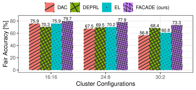
We now present the performance of Facade and the baselines w.r.t. the fair accuracy metric given by Equation 6. To compute this metric, we use $\lambda=\nicefrac{{2}}{{3}}$, as it slightly favors well-performing models while still giving significant weight to penalizing large discrepancies. We use a similar experiment setup as in Section V-B and measure the fair accuracy periodically throughout the model training.

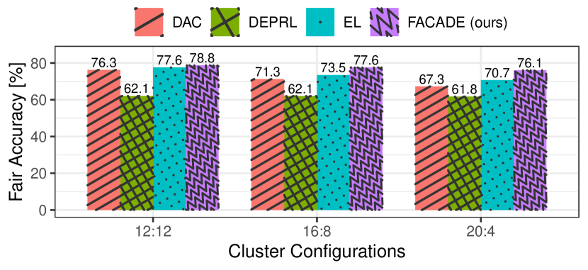
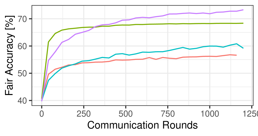
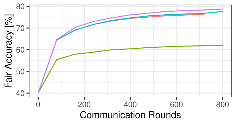
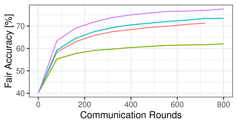
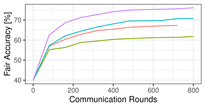
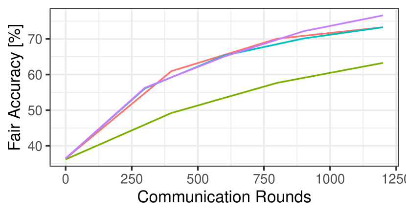
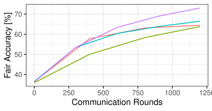
Figure 5 illustrates the highest obtained fair accuracy for each evaluated algorithm and cluster configuration, for both the CIFAR-10 and Imagenette datasets. Figure 5(a) shows that Facade achieves the highest fair accuracy for all cluster configurations compared to baseline approaches. For the 30:2 cluster configuration, Facade achieves 73.3% fair accuracy, whereas the second-best baseline, DePRL, achieves 68.4% fair accuracy. In contrast, EL shows a lower fair accuracy of 60.8%. This result underlines that Facade both achieves high model accuracy and minimizes the performance differences between groups. The same trend holds for the Imagenette dataset, shown in Figure 5(b). For the 20:4 cluster configuration, Facade achieves 76.1% fair accuracy, compared to 70.7% fair accuracy for EL. The fair accuracy for Flickr-Mammals is provided in Appendix D and is consistent with the findings for the CIFAR-10 and Imagenette datasets. We provide additional fair accuracy plots in Appendix C, showing how the fair accuracy evolves throughout the training process.

(a) CIFAR-10

(b) Imagenette

Figure 6: Boxplot of demographic parity (left, $\downarrow$ is better) and equalized odds (right, $\downarrow$ is better) obtained on CIFAR-10 and Imagenette, for varying cluster configurations and algorithms.

V-D Per-cluster fairness for varying cluster configurations

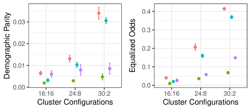
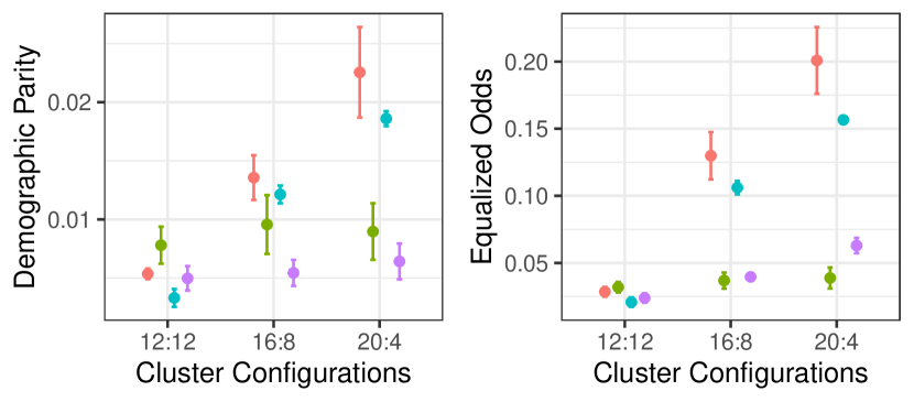
We measure the demographic parity (DP) and equalized odds (EO) metrics on the final model of each experiment conducted in the previous section. For this, we use Equation 1 and Equation 2 that were introduced in Section II-B. These results are visualized in Figure 6, showing the DP and EO for different cluster configurations, algorithms, and for the CIFAR-10 and Imagenette datasets.

Figure 6 shows that when cluster sizes are equal (, 16:16 for CIFAR-10 and 12:12 for Imagenette), the DP and EO of all algorithms is comparable. When the cluster sizes become more unbalanced, Facade exhibits lower DP and EO compared to EL and DAC. The only baseline that outperforms Facade is DePRL, which exhibits lower DP and EO. However, regardless of cluster membership, the accuracy for all nodes with DePRL is lower, particularly for Imagenette (see Figure 4), which can misleadingly be interpreted as having good fairness. We notice that model heads in DePRL overfit significantly on the nodes’ local data because it is never shared with other nodes. Consequently, the algorithm cannot leverage the similar data distribution of other nodes and struggles to generalize on the test set. This example motivates the fair accuracy metric we introduced in Section V-C1. Considering the low accuracy of DePRL, we conclude that Facade results in fairer treatment of minority clusters when cluster sizes are heavily unbalanced.

V-E Communication cost of Facade and baselines

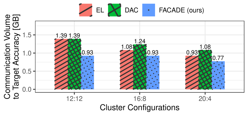
We now quantify the communication cost of Facade and baselines to reach a target accuracy. We set this target accuracy to 63% and 65% for the CIFAR-10 and Imagenette datasets, respectively, which is the lowest accuracy by any baseline reached after $T=1200$. We exclude DePRL from this experiment due to its inferior performance compared to Facade and other baselines. In contrast to the previous experiments, we consider the average accuracy of the entire network and not the per-cluster performance.

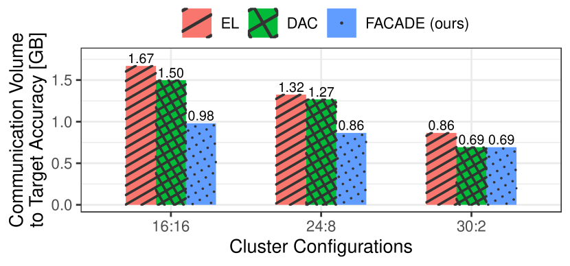
Figure 7 illustrates the communication cost in GB required to reach the target accuracy for each cluster configuration and different algorithms for the CIFAR-10 and Imagenette datasets. Figure 7(a) shows these results for CIFAR-10. In the 16:16 cluster configuration, Facade requires 41.3% and 34.6% less communication volume to reach the target accuracy compared to EL and DAC, respectively. This reduction is less pronounced for the 30:2 cluster configuration, with Facade requiring near-equal communication cost as DAC. Figure 7(b) shows the communication volume required to reach the target accuracy for Imagenette. In all cluster configurations, Facade requires less communication volume than EL and DAC. In the 16:16 cluster configuration, Facade requires 33.3% less communication volume to reach the target accuracy than both EL and DAC. This reduction becomes 16.6% and 28.5% in the 20:4 cluster configuration compared to EL and DAC, respectively.

From an algorithmic perspective, the communication cost of Facade per round is the same as that of EL or D-PSGD. Specifically, in each round, a node in Facade also sends only one model to each neighbor. However, each model transfer includes an additional integer that indicates the model head index. The overhead of this additional integer on the total communication volume is negligible. Yet, Facade can reach the target accuracy faster than or equally fast as baselines.

(a) CIFAR-10 (target test accuracy: 63%)

(b) Imagenette (target test accuracy: 65%)

Figure 7: Communication volume (in GB) required to reach a target test accuracy on the CIFAR-10 and Imagenette datasets, for different cluster configurations and algorithms ($\downarrow$ is better).

V-F The effect of $k$ on per-cluster test accuracy

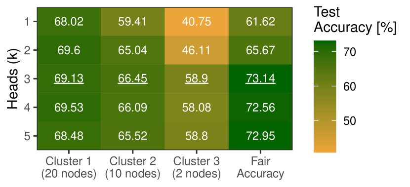
Facade introduces a hyperparameter $k$, which defines the number of model heads each node maintains. Ideally, $k$ should match the number of unique features in the dataset, which can be difficult to estimate beforehand without sharing data. We evaluate the sensitivity of Facade to variations in $k$. We create three clusters with 20, 10, and 2 nodes in a 32-node network and use the CIFAR-10 dataset. Each cluster has images rotated by 0°, 90°, and 180°, respectively. This experiment also demonstrates the capacity of Facade to handle more than two clusters. We vary the number of model heads from one to five.

Figure 8 shows the per-cluster test accuracy (columns) while varying $k$ (rows). We also show the fair accuracy in the right-most column. When only one model head is used ($k=1$), Facade is equivalent to EL. However, $k=1$ shows poor test accuracy (40.75%) for the minority cluster with only two nodes. In the configuration with two model heads, two clusters tend to share a head, while the remaining cluster has a dedicated model head that is specialized for its data distribution. Using three model heads demonstrates the best performance for each cluster, except for the majority cluster. This is expected as we augmented the data with three clusters of features. Nevertheless, even when using four and five model heads, the attained model utility is remarkably close to those obtained with the optimal number of heads. We observe that for $k>3$, multiple heads tend to specialize for the same cluster, often the largest one.

This experiment highlights the robustness of our algorithm to variations of the hyperparameter $k$. The system maintains a performance level close to the optimum, showcasing its resilience. Figure 8 reveals that it is better to overestimate than to underestimate the value of $k$. However, in practical settings, there may be guidelines to estimate $k$, , the number of data sources used to obtain the training data.

Figure 8: Highest attained test accuracy of Facade with a varying number of model heads for different clusters (left, $\uparrow$ is better). The average accuracies achieved by all nodes within each cluster are reported. We also report the fair accuracy in the right-most column.

V-G Facade cluster assignment

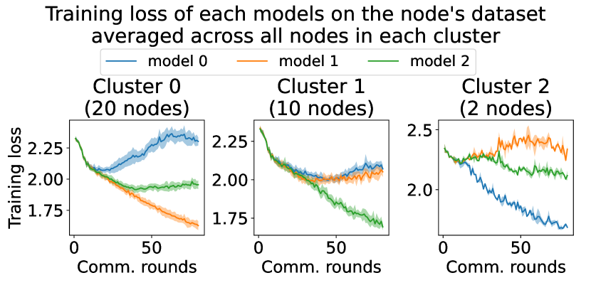
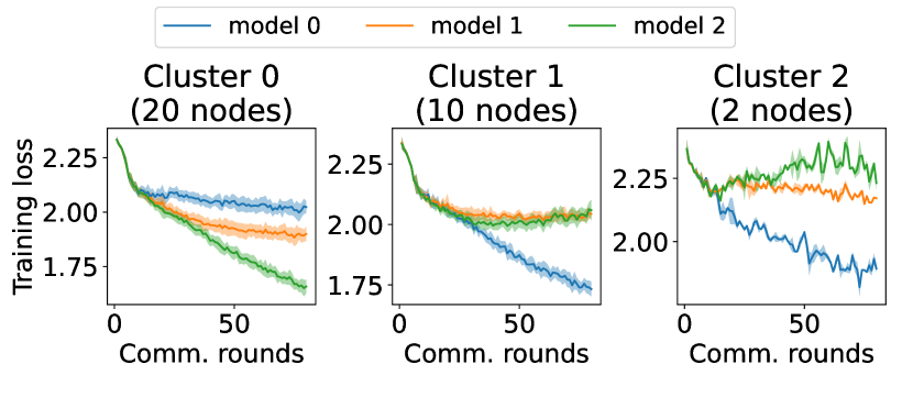
Finally, we analyze how nodes in Facade gravitate towards a particular cluster throughout the training process. We use the same three-cluster setup as the experiment in Section V-F and focus on the CIFAR-10 dataset. We record for each node the cluster it belongs to and the model head index it selects during each communication round.

Figure 9 shows the distribution of model head selection by nodes in each cluster during the first $80$ communication round. At the start, we have a fuzzy phase where nodes tend to explore different heads across rounds. The nodes in the minority cluster converge quicker and pick the same model head just after $18$ rounds. After about $42$ rounds, all nodes in the same cluster converge to the same head. This shows that nodes in each cluster in Facade quickly converge to the same model head, compared to the total training duration ($1200$ rounds).

During our experiments, we observed runs in which some nodes within the same cluster did not favor the same model head, or some model heads had not been selected at all. We attribute this to variance in the obtained training losses during the early stages of the learning process. We point out that similar behavior has been reported by related work on clustered federated learning [36]. Nevertheless, we found such failures in cluster assignment to be a rare occurrence (Appendix E).

(a) Cluster 1 (20 nodes)

(b) Cluster 2 (10 nodes)

(c) Cluster 3 (2 nodes)

Figure 9: The distribution of model head selection by nodes in each of the three clusters during the first $80$ communication round, using the CIFAR-10 dataset.

VI Related Work

We next discuss related work in the field of CML.

VI-A Personalized learning

Facade can be seen as a form of personalized learning to realize per-cluster models with fair treatment for minority groups. Personalization in the context of CML involves training different models that are personalized for groups or individual nodes [47]. In contrast, the objective of standard CML algorithms such as FedAvg is to train a single, global model that meets the demands of all users. Personalization can, for example, be used to deal with heterogeneous data distributions, where personalization can increase model utility across various subsets of the network compared to when using non-personalized approaches [48, 49, 50].

Personalization is a popular research avenue in FL. A prominent personalization approach involves each node maintaining a personal model, in addition to training a global one [51, 52, 53, 54].

Similar to Facade, some other personalization techniques also involve nodes sharing only the core of their model with the server, while the personalized head is kept and learns to fit the local data [55, 56, 36]. When the union of nodes’ training data naturally forms clusters, some FL techniques first partition these nodes accordingly before learning a separate model for each of them [57, 58, 59]. A key difference between the work as mentioned above and Facade is that personalization in FL is generally an easier problem to address than in a decentralized setting, as the server can collect global statistics and orchestrate the learning process. Furthermore, in contrast to our work, none of the previously mentioned works focus on fairness.

In DL, early work on personalized learning incorporates a notion of similarity between nodes when constructing the communication topology [60, 61]. These approaches assume the availability of a similarity matrix, which is often unavailable. In DL, where privacy is a major concern, the data needed to determine the similarity between nodes typically cannot be shared. Other methods leverage a dynamic network to enhance personalization, where neighbors are dynamically selected, based on some performance metric, throughout the training process [62, 12]. L2C, for example, uses an attention mechanism to automatically assign mixing weights by comparing two nodes’ model updates [62]. Facade, however, relies on unbiased, randomized communication and refreshes the topology each training round. Personalization has also been used to reduce the communication cost of DL, , DisPFL employs personalized sparse masks to customize sparse local models on the edge [63]. DePRL is a state-of-the-art personalized DL algorithm that allows each node to optimize its model head locally while sharing the core model through periodic communication and aggregation steps [11].

Compared to Facade, most existing personalization methods focus on personalization at the node level and do not leverage similarities when dealing with clustered data. Additionally, these algorithms often focus on achieving high model utility and do not focus on fairness.

VI-B Fairness in CML

The objective of fairness-aware approaches in CML usually is to ensure equal model performance for all participants in the network. The fairness objective in the work of Du et al. [64] is to ensure that predictions made by the global model are fair across different clients, regardless of variations in local data distributions. Similar to Facade, they apply DP as a fairness metric but operate in a centralized setting. Chen et al. [65] propose a fairness-aware decentralized learning framework that uses a custom aggregation scheme, taking into consideration the local learning objective and preferences. FairFed [25] is a FL algorithm designed to enhance group fairness through a fairness-aware aggregation strategy. To the best of our knowledge, we are the first to study fairness across different demographic groups in decentralized learning.

VI-C Other forms of data heterogeneity

Facade is designed to achieve fairness in settings with feature heterogeneity. In DL, data heterogeneity may also arise from skewed label distributions or differences in the sizes of local datasets. Dynamic topologies have been shown to allow better mixing of models in the presence of skewed label distributions [3]. Skewscout [41] reduces the communication cost in DL in the presence of data heterogeneity. In contrast, Facade tries to optimize both fairness and accuracy of the models. We believe Facade is general enough to incorporate solutions like Skewscout to achieve fairness at lower communication costs. However, communication cost is an orthogonal problem and Facade does not increase the communication cost compared to DL algorithms such as EL or D-PSGD.

VII Conclusion

In this paper, we introduced Facade, a DL algorithm designed to address fairness issues in network with feature heterogeneity. By maintaining multiple model heads at each node, Facade personalizes models for different data clusters, ensuring fairness and high model utility across different groups. Through a comprehensive evaluation with three state-of-the-art baselines and datasets, we demonstrated that Facade achieves high accuracy, particularly benefiting minority groups, without increasing communication costs. Facade thus offers a robust solution for DL in scenarios with feature heterogeneity, combining fairness and model accuracy.

Appendix A Proofs

Proof of Theorem 1

From the perspective of a fixed node $N_{i}$, we can draw the same line of reasoning as in Theorem 2 and Lemma 3 of [36]. ∎

Proof of Theorem 2

Fix any cluster $j\in[k]$ and a round $t>0$. Firstly, we observe that

$$\norm{\theta^{[j](t+1)}-\theta^{*}_{[j]}}=\norm{\left(\frac{1}{|S^{(t)}_{[j]}|}\sum_{i\in S_{[j]}^{(t)}}\bar{\theta}_{i}^{[j](t+1)}\right)-\theta^{*}_{[j]}}$$

$$=\norm{\frac{1}{|S^{(t)}_{[j]}|}\sum_{i\in S_{[j]}^{(t)}}\left(\bar{\theta}_{i}^{[j](t+1)}-\theta^{*}_{[j]}\right)}$$

$$\leq\frac{1}{|S^{(t)}_{[j]}|}\sum_{i\in S_{[j]}^{(t)}}\norm{\bar{\theta}_{i}^{[j](t+1)}-\theta^{*}_{[j]}}\text{ [triangle inequality]}$$ (7)

From (7), we conclude that for any $\zeta>0$, we have:

$$\mathbb{P}\left[\norm{\bar{\theta}^{[j](t+1)}-\theta^{*}_{[j]}}\leq\zeta\right]$$

$$\geq\mathbb{P}\left[\frac{1}{|S^{(t)}_{[j]}|}\sum_{i\in S_{[j]}^{(t)}}\norm{\bar{\theta}_{i}^{[j](t+1)}-\theta^{*}_{[j]}}\leq\zeta\right]$$

$$=\mathbb{P}\left[\sum_{i\in S_{[j]}^{(t)}}\norm{\bar{\theta}_{i}^{[j](t+1)}-\theta^{*}_{[j]}}\leq|S^{(t)}_{[j]}|\zeta\right]$$

$$\geq\mathbb{P}\left[\bigcap_{i\in S_{[j]}^{(t)}}\norm{\bar{\theta}_{i}^{[j](t+1)}-\theta^{*}_{[j]}}\leq\zeta\right]$$

$$=\prod_{i\in S_{[j]}^{(t)}}\mathbb{P}\left[\norm{\bar{\theta}_{i}^{[j](t+1)}-\theta^{*}_{[j]}}\leq\zeta\right]$$ (8)

$$[\because\,\text{$\bar{\theta}_{1}^{[j](t+1)},\ldots,\bar{\theta}_{n}^{[j](t+1)}$\, are pairwise-independent}]$$

Setting $\zeta=(1-\frac{p\lambda}{8L})\norm{\theta_{i}^{[j](t)}-\theta^{*}_{[j]}}+\epsilon_{0}$ and using Theorem 1, we conclude the proof. ∎

Proof of Corollary 3

Using Theorem 2, the proof follows the identical line of reasoning as that of Corollary 2 of [36]. ∎

Appendix B D-PSGD Pseudocode

We show in Algorithm 1 the standard D-PSGD procedure from the perspective of node $i$.

1 Initialize $\theta_{i}^{(0)}$

2 for $t=0,\dots,T-1$ do

3       $\tilde{\theta}_{i}^{(t,0)}\leftarrow\theta_{i}^{(t)}$

4       for $h=0,\dots,H-1$ do

5             $\xi_{i}\leftarrow$ mini-batch sampled from $D_{i}$

6             $\tilde{\theta}_{i}^{(t,h+1)}\leftarrow\tilde{\theta}_{i}^{(t,h)}-\eta\nabla f_{i}(\tilde{\theta}_{i}^{(t,h)},\xi_{i})$

7            

8       Send $\tilde{\theta}_{i}^{(t,H)}$ to the neighbors in topology $\mathcal{G}$

9       Receive $\tilde{\theta}_{j}^{(t,H)}$ from each neighbor $j$ in $\mathcal{G}$

10       Aggregate the received models to produce $\theta_{i}^{(t+1)}$

11      

12return $\theta_{i}^{(T)}$

Algorithm 1 The D-PSGD procedure, from the perspective of node $i$.

(a) 16:16 cluster configuration

(b) 24:8 cluster configuration

(c) 30:2 cluster configuration

Figure 10: Fair Accuracy ($\uparrow$ is better) obtained on CIFAR-10.

(a) 12:12 cluster configuration

(b) 16:8 cluster configuration

(c) 20:4 cluster configuration

Figure 11: Fair Accuracy ($\uparrow$ is better) obtained on Imagenette.

(a) 8:8 cluster configuration

(b) 14:2 cluster configuration

Figure 12: Fair Accuracy ($\uparrow$ is better) obtained on FLICKR.

Appendix C Additional fair accuracy plots

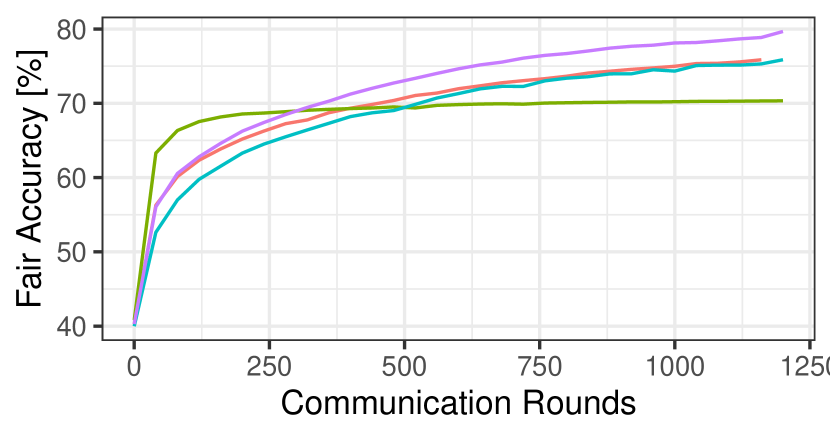
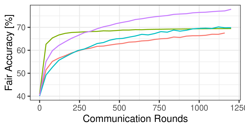
Figure 10, Figure 11 and Figure 12 provide the evolution of fair accuracy for varying cluster configurations and the CIFAR-10, Imagenette, and Flickr-Mammals datasets, respectively. To compute the fair accuracy, we use $\alpha=\nicefrac{{2}}{{3}}$. We observe that for all datasets and cluster configurations, Facade achieves the highest fair accuracy.

(a) 8:8 cluster configuration

(b) 14:2 cluster configuration

Figure 13: Average test accuracy for the nodes in the majority cluster (left) and those in the minority (right) obtained on Flickr-Mammals ($\uparrow$ is better), for different cluster configurations.

Appendix D Experimental results for the Flickr-Mammals dataset

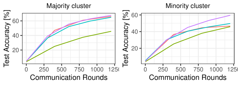
In this section, we provide additional plots for the more challenging Flickr-Mammals dataset. Figure 13 shows the average test accuracy for the majority and minority clusters, for different cluster configurations and on the Flickr-Mammals dataset. Figure 13(a) reveals that Facade for a 8:8 cluster configuration after $T=1200$ reaches higher test accuracy than baselines, both for the minority and majority cluster. Figure 13(b) shows that for a 14:2 cluster configuration, Facade achieves comparable test accuracy for the majority cluster but shows a significant improvement in test accuracy for the minority cluster: 49.7% for EL against 59.6% for Facade.

Figure 14: Highest observed fair accuracy for Flickr-Mammals, for varying cluster configurations and algorithms ($\uparrow$ is better). To compute the fair accuracy, we use $\alpha=\nicefrac{{2}}{{3}}$.

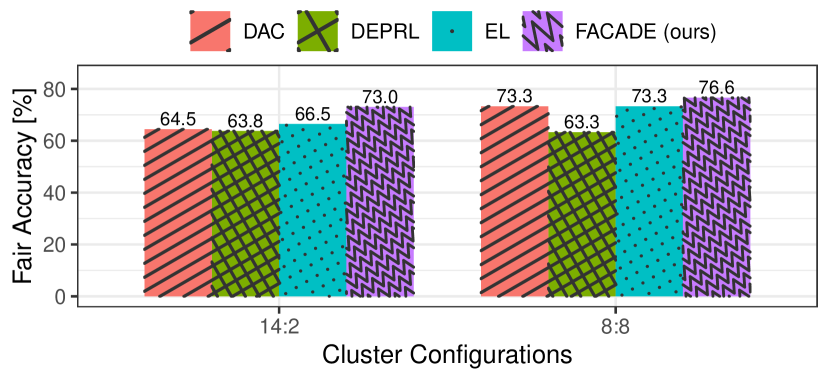
Figure 14 shows the fair accuracy obtained on the Flickr-Mammals dataset, for varying cluster configurations and algorithms. In both cluster configurations, Facade achieves the highest fair accuracy. This is in line with the results reported in Section V-C for the other datasets.

Figure 15: Boxplot of demographic parity (left, $\downarrow$ is better) and equalized odds (right, $\downarrow$ is better) obtained on Flickr-Mammals, for varying cluster configurations and algorithms.

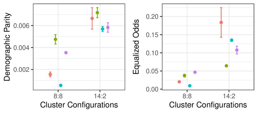
Figure 15 shows the DP and EO obtained on Flickr-Mammals, for varying cluster configurations and algorithms. Facade shows comparable DP performance to EL in an 8:8 cluster configuration. However, Facade achieves a lower EO score EO than EL and DAC in a 14:2 cluster configuration. In the same configuration, DePRL achieves the lowest EO score, which is in line with the results reported in Section V-D.

TABLE II: Summary of experimental results on the CIFAR-10 dataset.

Config	Algorithm	Accmaj$\uparrow$	Accmin $\uparrow$	Accall $\uparrow$	Demo. Par. $\downarrow$	Equ. Odds $\downarrow$	Accfair $\uparrow$
16:16	EL	64.03$\pm$0.54	63.80$\pm$0.42	63.91$\pm$0.43	0.0032$\pm$0.0007	0.0204$\pm$0.0038	75.87
	DAC	63.82$\pm$1.34	63.79$\pm$1.43	63.81$\pm$0.31	0.0065$\pm$0.0008	0.0402$\pm$0.0057	75.86
	DePRL	55.51$\pm$0.34	55.50$\pm$0.29	55.50$\pm$0.26	0.0020$\pm$0.0004	0.0099$\pm$0.0026	70.33
	FACADE	69.50$\pm$0.32	69.61$\pm$0.20	69.55$\pm$0.25	0.0060$\pm$0.0015	0.0267$\pm$0.0079	79.67
24:8	EL	69.13$\pm$0.45	54.76$\pm$0.59	65.53$\pm$0.31	0.0103$\pm$0.0012	0.1596$\pm$0.0097	69.84
	DAC	69.88$\pm$0.28	51.30$\pm$1.31	65.24$\pm$0.19	0.0131$\pm$0.0015	0.2067$\pm$0.0175	67.53
	DePRL	57.40$\pm$0.13	54.21$\pm$0.24	56.60$\pm$0.15	0.0030$\pm$0.0003	0.0361$\pm$0.0013	69.48
	FACADE	71.61$\pm$0.27	66.81$\pm$0.34	70.41$\pm$0.29	0.0079$\pm$0.0025	0.0582$\pm$0.0033	77.87
30:2	EL	71.99$\pm$0.70	38.77$\pm$0.62	69.91$\pm$0.67	0.0306$\pm$0.0014	0.3693$\pm$0.0081	59.18
	DAC	72.21$\pm$0.24	34.94$\pm$0.72	69.88$\pm$0.25	0.0340$\pm$0.0027	0.4143$\pm$0.0075	56.63
	DePRL	58.47$\pm$0.59	52.56$\pm$0.78	58.10$\pm$0.57	0.0047$\pm$0.0013	0.0684$\pm$0.0072	68.37
	FACADE	73.32$\pm$0.15	59.96$\pm$0.72	72.48$\pm$0.19	0.0086$\pm$0.0026	0.1491$\pm$0.0059	73.31

TABLE III: Summary of experimental results on the Imagenette dataset.

Config	Algorithm	Accmaj$\uparrow$	Accmin $\uparrow$	Accall $\uparrow$	Demo. Par. $\downarrow$	Equ. Odds $\downarrow$	Accfair $\uparrow$
12:12	EL	66.43$\pm$0.56	66.85$\pm$0.67	66.64$\pm$0.59	0.0033$\pm$0.0008	0.0208$\pm$0.0035	77.62
	DAC	65.73$\pm$0.73	64.45$\pm$0.54	65.09$\pm$0.47	0.0054$\pm$0.0004	0.0286$\pm$0.0036	76.30
	DePRL	43.14$\pm$1.00	43.49$\pm$1.20	43.31$\pm$1.07	0.0078$\pm$0.0016	0.0319$\pm$0.0039	62.10
	FACADE	68.18$\pm$0.35	68.59$\pm$0.34	68.39$\pm$0.27	0.0050$\pm$0.0010	0.0239$\pm$0.0035	78.78
16:8	EL	69.69$\pm$0.27	60.21$\pm$0.44	67.32$\pm$0.29	0.0121$\pm$0.0008	0.1061$\pm$0.0050	73.48
	DAC	68.55$\pm$0.62	56.92$\pm$1.32	65.64$\pm$0.57	0.0136$\pm$0.0019	0.1299$\pm$0.0176	71.28
	DePRL	43.40$\pm$0.79	43.09$\pm$1.22	43.33$\pm$0.89	0.0096$\pm$0.0025	0.0361$\pm$0.0060	62.06
	FACADE	69.61$\pm$0.37	66.44$\pm$0.19	68.82$\pm$0.30	0.0054$\pm$0.0011	0.0397$\pm$0.0014	77.63
20:4	EL	70.17$\pm$0.28	56.06$\pm$0.56	67.81$\pm$0.33	0.0186$\pm$0.0006	0.1566$\pm$0.0026	70.71
	DAC	69.05$\pm$0.74	50.93$\pm$1.65	66.03$\pm$0.45	0.0226$\pm$0.0039	0.2009$\pm$0.0249	67.29
	DePRL	43.67$\pm$1.01	42.64$\pm$1.16	43.50$\pm$1.02	0.0090$\pm$0.0024	0.0388$\pm$0.0078	61.76
	FACADE	69.61$\pm$0.46	64.15$\pm$0.39	68.70$\pm$0.42	0.0064$\pm$0.0015	0.0630$\pm$0.0057	76.10

TABLE IV: Summary of experimental results on the Flickr-Mammals dataset.

Config	Algorithm	Accmaj$\uparrow$	Accmin $\uparrow$	Accall $\uparrow$	Demo. Par. $\downarrow$	Equ. Odds $\downarrow$	Accfair $\uparrow$
8:8	EL	59.97$\pm$0.23	59.92$\pm$0.22	59.94$\pm$0.19	0.0006$\pm$0.0001	0.0094$\pm$0.0014	73.28
	DAC	60.56$\pm$0.60	59.94$\pm$0.32	60.25$\pm$0.33	0.0016$\pm$0.0002	0.0203$\pm$0.0012	73.29
	DePRL	44.92$\pm$0.61	45.61$\pm$1.23	45.26$\pm$0.85	0.0047$\pm$0.0004	0.0373$\pm$0.0039	63.28
	FACADE	65.50$\pm$0.55	64.92$\pm$0.41	65.21$\pm$0.47	0.0035$\pm$0.0001	0.0467$\pm$0.0018	76.62
14:2	EL	64.92$\pm$0.21	49.71$\pm$0.20	63.02$\pm$0.17	0.0057$\pm$0.0002	0.1349$\pm$0.0034	66.47
	DAC	66.11$\pm$0.46	46.70$\pm$4.75	63.68$\pm$0.63	0.0067$\pm$0.0010	0.1836$\pm$0.0409	64.47
	DePRL	45.69$\pm$0.82	45.91$\pm$0.79	45.72$\pm$0.81	0.0072$\pm$0.0005	0.0644$\pm$0.0027	63.80
	FACADE	67.63$\pm$0.49	59.55$\pm$1.06	66.62$\pm$0.56	0.0058$\pm$0.0004	0.1077$\pm$0.0109	73.03

Appendix E Notes on Facade cluster assignment

We mentioned in Section V-G that Facade sometimes fails to assign nodes to the correct cluster. In this section, we provide additional insights into the concept of settlement in our algorithm. In Facade, a scenario can arise where one or more heads consistently outperform the others across all nodes. When this happens, only the superior heads are selected, causing the other heads to be ignored and never be updated throughout the learning session. This situation is referred to as the algorithm not settling. Figure 16 illustrates this behavior, with an example where Facade did settle (Figure 16(a) and another where it did not (Figure 16(b)).

We empirically observed that the probability of not settling is higher when the cluster sizes are more unbalanced. When the algorithm does not settle, it cannot fully exploit its potential and results in sub-optimal model utility and fairness. However, it is important to note that not settling is not a catastrophic issue. In such cases, performance in the worst case drops to the level of EL, and a simple change of seeds is usually enough to achieve settlement.

To mitigate the risk of not settling, we employ several strategies. First, with careful selection of model hyperparameters, we can reduce the likelihood of this occurrence. Another effective strategy is to initiate the training with a few rounds of EL, where all heads share the same weights before transitioning to independent parameters for each head. This initial shared training phase is particularly crucial during the early stages of the algorithm when the models are still largely predicting randomly. During this phase, one head can easily capture a better data representation and quickly outperform the others. By beginning with shared training, the core and heads develop a solid data representation foundation. When the heads eventually train independently, it becomes easier for each to specialize in a specific cluster’s data distribution, thus stabilizing the training process. These techniques proved effective in stabilizing the training process and enhancing the overall performance of Facade. By incorporating initial shared training, we significantly reduced the likelihood of the algorithm failing to settle, thereby maximizing its potential.

(a) Facade did settle

(b) Facade did not settle

Figure 16: The evolution of training loss ($\downarrow$ is better) on the shared core and each of the three model heads, averaged across nodes within the same cluster. The top plot illustrates a case where Facade successfully settled, meaning all nodes within the same cluster favor the same model, and no nodes of another cluster picked it. The bottom plot shows a case where the algorithm did not settle, resulting in all nodes from clusters 1 and 2 selecting and training the same model (model 0). We observe that model 1 is not selected at iteration 80, indicating it will no longer be chosen, as it will not be trained and thus will not improve on any distribution.

References

- [1] X. Lian, C. Zhang, H. Zhang, C.-J. Hsieh, W. Zhang, and J. Liu, “Can decentralized algorithms outperform centralized algorithms? a case study for decentralized parallel stochastic gradient descent,” Advances in neural information processing systems, vol. 30, 2017.
- [2] R. Ormándi, I. Hegedűs, and M. Jelasity, “Gossip learning with linear models on fully distributed data,” Concurrency and Computation: Practice and Experience, vol. 25, no. 4, pp. 556–571, 2013.
- [3] M. de Vos, S. Farhadkhani, R. Guerraoui, A.-M. Kermarrec, R. Pires, and R. Sharma, “Epidemic learning: Boosting decentralized learning with randomized communication,” in NeurIPS, 2023.
- [4] S. Caldas, S. M. K. Duddu, P. Wu, T. Li, J. Konečnỳ, H. B. McMahan, V. Smith, and A. Talwalkar, “Leaf: A benchmark for federated settings,” arXiv preprint arXiv:1812.01097, 2018.
- [5] N. Rieke, J. Hancox, W. Li, F. Milletari, H. R. Roth, S. Albarqouni, S. Bakas, M. N. Galtier, B. A. Landman, K. Maier-Hein et al., “The future of digital health with federated learning,” NPJ digital medicine, vol. 3, no. 1, pp. 1–7, 2020.
- [6] D. C. Nguyen, Q.-V. Pham, P. N. Pathirana, M. Ding, A. Seneviratne, Z. Lin, O. Dobre, and W.-J. Hwang, “Federated learning for smart healthcare: A survey,” ACM Computing Surveys (Csur), vol. 55, no. 3, pp. 1–37, 2022.
- [7] Y. LeCun, L. Bottou, Y. Bengio, and P. Haffner, “Gradient-based learning applied to document recognition,” Proceedings of the IEEE, vol. 86, no. 11, pp. 2278–2324, 1998.
- [8] A. Krizhevsky, G. Hinton et al., “Learning multiple layers of features from tiny images,” 2009.
- [9] D. Pessach and E. Shmueli, “A review on fairness in machine learning,” ACM Computing Surveys (CSUR), vol. 55, no. 3, pp. 1–44, 2022.
- [10] R. Berk, H. Heidari, S. Jabbari, M. Kearns, and A. Roth, “Fairness in criminal justice risk assessments: The state of the art,” Sociological Methods & Research, vol. 50, no. 1, pp. 3–44, 2021.
- [11] G. Xiong, G. Yan, S. Wang, and J. Li, “Deprl: Achieving linear convergence speedup in personalized decentralized learning with shared representations,” in Proceedings of the AAAI Conference on Artificial Intelligence, vol. 38, no. 14, 2024, pp. 16 103–16 111.
- [12] E. L. Zec, E. Ekblom, M. Willbo, O. Mogren, and S. Girdzijauskas, “Decentralized adaptive clustering of deep nets is beneficial for client collaboration,” in International Workshop on Trustworthy Federated Learning. Springer, 2022, pp. 59–71.
- [13] E. U. Soykan, L. Karaçay, F. Karakoç, and E. Tomur, “A survey and guideline on privacy enhancing technologies for collaborative machine learning,” IEEE Access, vol. 10, 2022.
- [14] D. Pasquini, M. Raynal, and C. Troncoso, “On the (in) security of peer-to-peer decentralized machine learning,” in 2023 IEEE Symposium on Security and Privacy (SP), 2023, pp. 418–436.
- [15] A. Nedić and A. Olshevsky, “Stochastic gradient-push for strongly convex functions on time-varying directed graphs,” IEEE Transactions on Automatic Control, vol. 61, no. 12, 2016.
- [16] M. Assran, N. Loizou, N. Ballas, and M. Rabbat, “Stochastic gradient push for distributed deep learning,” in ICML, 2019.
- [17] Y. Lu, Z. Yu, and N. Suri, “Privacy-preserving decentralized federated learning over time-varying communication graph,” ACM Transactions on Privacy and Security, vol. 26, no. 3, pp. 1–39, 2023.
- [18] B. McMahan, E. Moore, D. Ramage, S. Hampson, and B. A. y Arcas, “Communication-efficient learning of deep networks from decentralized data,” in Artificial intelligence and statistics. PMLR, 2017, pp. 1273–1282.
- [19] N. Mehrabi, F. Morstatter, N. Saxena, K. Lerman, and A. Galstyan, “A survey on bias and fairness in machine learning,” ACM computing surveys (CSUR), vol. 54, no. 6, pp. 1–35, 2021.
- [20] S. Verma and J. Rubin, “Fairness definitions explained,” in Proceedings of the international workshop on software fairness, 2018, pp. 1–7.
- [21] R. Hanna and L. Linden, “Measuring discrimination in education,” National Bureau of Economic Research, Tech. Rep., 2009.
- [22] K. Makhlouf, S. Zhioua, and C. Palamidessi, “On the applicability of machine learning fairness notions,” ACM SIGKDD Explorations Newsletter, vol. 23, no. 1, pp. 14–23, 2021.
- [23] C. Dwork, M. Hardt, T. Pitassi, O. Reingold, and R. Zemel, “Fairness through awareness,” in Proceedings of the 3rd innovations in theoretical computer science conference, 2012, pp. 214–226.
- [24] M. Hardt, E. Price, and N. Srebro, “Equality of opportunity in supervised learning,” Advances in neural information processing systems, vol. 29, 2016.
- [25] Y. H. Ezzeldin, S. Yan, C. He, E. Ferrara, and A. S. Avestimehr, “Fairfed: Enabling group fairness in federated learning,” in Proceedings of the AAAI conference on artificial intelligence, vol. 37, no. 6, 2023, pp. 7494–7502.
- [26] K. Jung, S. Biswas, and C. Palamidessi, “Establishing the price of privacy in federated data trading,” in Protocols, Strands, and Logic: Essays Dedicated to Joshua Guttman on the Occasion of his 66.66 th Birthday. Springer, 2021, pp. 232–250.
- [27] C. Denis, R. Elie, M. Hebiri, and F. Hu, “Fairness guarantees in multi-class classification with demographic parity,” Journal of Machine Learning Research, vol. 25, no. 130, pp. 1–46, 2024.
- [28] J. Rouzot, J. Ferry, and M. Huguet, “Learning optimal fair scoring systems for multi-class classification,” in 2022 IEEE 34th International Conference on Tools with Artificial Intelligence (ICTAI). Los Alamitos, CA, USA: IEEE Computer Society, nov 2022, pp. 197–204.
- [29] E. T. M. Beltrán, M. Q. Pérez, P. M. S. Sánchez, S. L. Bernal, G. Bovet, M. G. Pérez, G. M. Pérez, and A. H. Celdrán, “Decentralized federated learning: Fundamentals, state of the art, frameworks, trends, and challenges,” IEEE Communications Surveys & Tutorials, 2023.
- [30] C. Shiranthika, P. Saeedi, and I. V. Bajić, “Decentralized learning in healthcare: a review of emerging techniques,” IEEE Access, vol. 11, 2023.
- [31] J. R. Douceur, “The sybil attack,” in International workshop on peer-to-peer systems. Springer, 2002.
- [32] A. Antonov and S. Voulgaris, “Securecyclon: Dependable peer sampling,” in 2023 IEEE 43rd International Conference on Distributed Computing Systems (ICDCS). IEEE, 2023, pp. 1–12.
- [33] R. Guerraoui, A.-M. Kermarrec, A. Kucherenko, R. Pinot, and M. de Vos, “Peerswap: A peer-sampler with randomness guarantees,” in Proceedings of the 43rd International Symposium on Reliable Distributed Systems (SRDS 2024), 2024.
- [34] J. MacQueen et al., “Some methods for classification and analysis of multivariate observations,” in Proceedings of the fifth Berkeley symposium on mathematical statistics and probability, vol. 1, no. 14. Oakland, CA, USA, 1967, pp. 281–297.
- [35] D. A. Reynolds et al., “Gaussian mixture models.” Encyclopedia of biometrics, vol. 741, no. 659-663, 2009.
- [36] A. Ghosh, J. Chung, D. Yin, and K. Ramchandran, “An efficient framework for clustered federated learning,” in Proceedings of the 34th International Conference on Neural Information Processing Systems, ser. NIPS ’20. Red Hook, NY, USA: Curran Associates Inc., 2020.
- [37] E. Cyffers, M. Even, A. Bellet, and L. Massoulié, “Muffliato: Peer-to-peer privacy amplification for decentralized optimization and averaging,” Advances in Neural Information Processing Systems, vol. 35, pp. 15 889–15 902, 2022.
- [38] S. Biswas, M. Even, A.-M. Kermarrec, L. Massoulie, R. Pires, R. Sharma, and M. de Vos, “Noiseless privacy-preserving decentralized learning,” arXiv preprint arXiv:2404.09536, 2024.
- [39] S. Biswas, D. Frey, R. Gaudel, A.-M. Kermarrec, D. Lerévérend, R. Pires, R. Sharma, and F. Taïani, “Low-cost privacy-aware decentralized learning,” arXiv preprint arXiv:2403.11795, 2024.
- [40] J. Howard, “Imagenette.” [Online]. Available: https://github.com/fastai/imagenette/
- [41] K. Hsieh, A. Phanishayee, O. Mutlu, and P. Gibbons, “The non-iid data quagmire of decentralized machine learning,” in International Conference on Machine Learning. PMLR, 2020, pp. 4387–4398.
- [42] K. He, X. Zhang, S. Ren, and J. Sun, “Deep residual learning for image recognition,” in Proceedings of the IEEE conference on computer vision and pattern recognition, 2016, pp. 770–778.
- [43] A. Dhasade, A.-M. Kermarrec, R. Pires, R. Sharma, and M. Vujasinovic, “Decentralized learning made easy with decentralizepy,” in Proceedings of the 3rd Workshop on Machine Learning and Systems, 2023, pp. 34–41.
- [44] J. Deng, W. Dong, R. Socher, L.-J. Li, K. Li, and L. Fei-Fei, “Imagenet: A large-scale hierarchical image database,” in 2009 IEEE conference on computer vision and pattern recognition. Ieee, 2009, pp. 248–255.
- [45] D. Lopez-Paz and M. Ranzato, “Gradient episodic memory for continual learning,” Advances in neural information processing systems, vol. 30, 2017.
- [46] P. Patarasuk and X. Yuan, “Bandwidth optimal all-reduce algorithms for clusters of workstations,” Journal of Parallel and Distributed Computing, vol. 69, no. 2, pp. 117–124, 2009.
- [47] V. Kulkarni, M. Kulkarni, and A. Pant, “Survey of personalization techniques for federated learning,” in 2020 fourth world conference on smart trends in systems, security and sustainability (WorldS4). IEEE, 2020, pp. 794–797.
- [48] X. Ma, J. Zhu, Z. Lin, S. Chen, and Y. Qin, “A state-of-the-art survey on solving non-iid data in federated learning,” Future Generation Computer Systems, vol. 135, pp. 244–258, 2022.
- [49] A. Z. Tan, H. Yu, L. Cui, and Q. Yang, “Towards personalized federated learning,” IEEE Transactions on Neural Networks and Learning Systems, 2022.
- [50] Q. Li, Y. Diao, Q. Chen, and B. He, “Federated learning on non-iid data silos: An experimental study,” in 2022 IEEE 38th international conference on data engineering (ICDE). IEEE, 2022, pp. 965–978.
- [51] Y. Huang, L. Chu, Z. Zhou, L. Wang, J. Liu, J. Pei, and Y. Zhang, “Personalized cross-silo federated learning on non-iid data,” in Proceedings of the AAAI conference on artificial intelligence, vol. 35, no. 9, 2021, pp. 7865–7873.
- [52] T. Li, S. Hu, A. Beirami, and V. Smith, “Ditto: Fair and robust federated learning through personalization,” in International conference on machine learning. PMLR, 2021, pp. 6357–6368.
- [53] M. Zhang, K. Sapra, S. Fidler, S. Yeung, and J. M. Alvarez, “Personalized federated learning with first order model optimization,” arXiv preprint arXiv:2012.08565, 2020.
- [54] Y. Mansour, M. Mohri, J. Ro, and A. T. Suresh, “Three approaches for personalization with applications to federated learning,” arXiv preprint arXiv:2002.10619, 2020.
- [55] L. Collins, H. Hassani, A. Mokhtari, and S. Shakkottai, “Exploiting shared representations for personalized federated learning,” in International conference on machine learning. PMLR, 2021, pp. 2089–2099.
- [56] R. Caruana, “Multitask learning,” Machine learning, vol. 28, pp. 41–75, 1997.
- [57] F. Sattler, K.-R. Müller, and W. Samek, “Clustered federated learning: Model-agnostic distributed multitask optimization under privacy constraints,” IEEE transactions on neural networks and learning systems, vol. 32, no. 8, pp. 3710–3722, 2020.
- [58] Y. Luo, X. Liu, and J. Xiu, “Energy-efficient clustering to address data heterogeneity in federated learning,” in ICC 2021-IEEE International Conference on Communications. IEEE, 2021, pp. 1–6.
- [59] D. K. Dennis, T. Li, and V. Smith, “Heterogeneity for the win: One-shot federated clustering,” in International Conference on Machine Learning. PMLR, 2021, pp. 2611–2620.
- [60] P. Vanhaesebrouck, A. Bellet, and M. Tommasi, “Decentralized collaborative learning of personalized models over networks,” in Artificial Intelligence and Statistics. PMLR, 2017, pp. 509–517.
- [61] A. Bellet, R. Guerraoui, M. Taziki, and M. Tommasi, “Personalized and private peer-to-peer machine learning,” in International conference on artificial intelligence and statistics. PMLR, 2018, pp. 473–481.
- [62] S. Li, T. Zhou, X. Tian, and D. Tao, “Learning to collaborate in decentralized learning of personalized models,” in Proceedings of the IEEE/CVF Conference on Computer Vision and Pattern Recognition, 2022, pp. 9766–9775.
- [63] R. Dai, L. Shen, F. He, X. Tian, and D. Tao, “Dispfl: Towards communication-efficient personalized federated learning via decentralized sparse training,” in International conference on machine learning. PMLR, 2022, pp. 4587–4604.
- [64] W. Du, D. Xu, X. Wu, and H. Tong, “Fairness-aware agnostic federated learning,” in Proceedings of the 2021 SIAM International Conference on Data Mining (SDM). SIAM, 2021, pp. 181–189.
- [65] Z. Chen, W. Liao, P. Tian, Q. Wang, and W. Yu, “A fairness-aware peer-to-peer decentralized learning framework with heterogeneous devices,” Future Internet, vol. 14, no. 5, p. 138, 2022.